Synchrony and the binding problem in macaque visual cortex

Abstract

We tested the binding-by-synchrony hypothesis which proposes that object representations are formed by synchronizing spike activity between neurons that code features of the same object. We studied responses of 32 pairs of neurons recorded with microelectrodes 3 mm apart in the visual cortex of macaques performing a fixation task. Upon mapping the receptive fields of the neurons, a quadrilateral was generated so that two of its sides were centered in the receptive fields at the optimal orientations. This one-figure condition was compared with a two-figure condition in which the neurons were stimulated by two separate figures, keeping the local edges in the receptive fields identical. For each neuron, we also determined its border ownership selectivity (H. Zhou, H. S. Friedman, & R. von der Heydt, 2000). We examined both synchronization and correlation at nonzero time lag. After correcting for effects of the firing rate, we found that synchrony did not depend on the binding condition. However, finding synchrony in a pair of neurons was correlated with finding border-ownership selectivity in both members of the pair. This suggests that the synchrony reflected the connectivity in the network that generates border ownership assignment. Thus, we have not found evidence to support the binding-by-synchrony hypothesis.

Introduction

Underlying the seemingly effortless perception of complex visual scenes are sophisticated neuronal computations that are necessary to extract information about the external world from an inherently ambiguous and frequently incomplete set of sensory inputs. One important component of this process is the organization of the visual scene into perceptual objects. At present, it is an unsolved question how the structure this imposes on the visual input is generated by the activity of neural assemblies.

One intriguing hypothesis is based on findings, made originally in the anesthetized cat (Eckhorn et al., 1988; Gray & Singer, 1989) but later also reported in the awake primate (Kreiter & Singer, 1992), that visual features that are linked together in perception are represented by groups of neurons that share coherent oscillations while the same neurons do not oscillate coherently in response to locally identical features that are not perceived as forming a group (von der Malsburg, 1981). While much emphasis was placed originally on the oscillatory nature of these activity patterns, more recently their synchronous nature has been considered the more functionally important aspect for distinguishing different parts of the same object (whose neural correlates would fire in synchrony) from parts of different objects (whose neural correlates would fire independently). Not all experimental evidence, however, supports this hypothesis. For instance, de Oliveira, Thiele, and Hoffmann (1997) recorded in dorsal extrastriate cortex of the awake macaque while the animal was performing a motion discrimination task. They found that synchrony did not convey information about the direction of motion of the stimuli and concluded that it is unlikely that synchrony information is used in their task. The “binding by synchrony” (BBS) hypothesis has been investigated in numerous other experimental and theoretical studies; for a recent review and more references to this literature, see Singer (2007). One possible extension of BBS is that binding is coded by correlated spikes at finite (nonzero) time lags. In order to test this alternative hypothesis as well, we extended a synchrony measure used by Roelfsema, Lamme, and Spekreijse (2004) to nonzero lag correlations (see below).

Visual scenes are not only complex but vision faces the additional difficulty that the three-dimensional world needs to be mapped on two two-dimensional retinae. One of the consequences of this mapping is that the projections of physical objects onto the retina will overlap, or, in the language of visual perception, occlusions will occur. Straightforward geometry dictates that the objects closer to the observer occlude a more distant object and that therefore the border between the two is determined by the former; in other words, the border is “owned” by the occluder. Recent physiological results (Qiu & von der Heydt, 2005; Zhou, Friedman, & von der Heydt, 2000) show that this relationship is represented in the firing properties of neurons as early as primary visual cortex, area V1, but more common in secondary visual cortex, area V2.

It has been observed both in biological systems and in computational models of varying complexity that different levels of correlation in the input to pairs of neurons result not only in different levels of pairwise correlation in their output but also in differences of their mean firing rates (e.g., Bernander & Koch, 1994; de la Rocha, Doiron, Shea-Brown, Josic, & Reyes, 2007; Mikula & Niebur, 2005). Thus, pairwise correlations between spike trains and mean firing rates are not independent. In order to eliminate this potentially confounding factor, we tested the dependence of synchronization on binding condition, border ownership, and firing rates simultaneously. As we will show, we did not observed a dependence of synchronization on the binding condition. However, a relation between synchrony and border ownership (BO) emerges which becomes understandable in the light of a recent computational model.

Materials and methods

We studied neurons in two adult macaque monkeys (Macaca mulatta). The details of our general experimental methods have been described (Qiu & von der Heydt, 2005; Zhou et al., 2000). The animals were prepared by implanting, under general anesthesia, first three small posts for head fixation, and later two recording chambers (one over each hemisphere). Fixation training was achieved by controlling fluid intake and using small amounts of juice or water to reward correct responses. All animal procedures conformed to National Institutes of Health and USDA guidelines as verified by the Animal Care and Use Committee of the Johns Hopkins University.

Stimuli and behavioral paradigm

Stimuli were generated on a Silicon Graphics O2 workstation using the antialiasing feature of the Open Inventor software, and presented on a Barco CCID 121 FS color monitor with a 72-Hz refresh rate. Stereoscopic pairs were presented side-by-side and superimposed optically at 40 cm viewing distance. The field of view subtended 17 by 26 deg visual angle. A background luminance of 16 cd/m² was used, except for conditions in border ownership tests in which figure and background color were flipped (see below). Eye movements were recorded for one eye using an infrared video based system (Iscan ETL-200) with a resolution of 5120 (H) and 2560 (V). The eye was imaged through a hot mirror (selectively reflecting infrared), with the camera placed on the axis of fixation. The optical magnification in our system resulted in a resolution of the pupil position signal of 0.03 deg visual angle in the horizontal and 0.06 deg in the vertical. However, noise and drifts of the signal reduced its accuracy.

Visual test stimuli were presented during periods of fixation. To achieve reliable fixation, the monkeys were trained to align a dot to a short line stereoscopically to within a disparity near the stereoscopic threshold. The criterion disparity was set so low that the adjustment took 1-2 seconds during which fixation was steady. Lateral movements during fixation were generally small (SD = 0.15-0.2 deg), and data from trials during which the fixation deviated from the target by more than 1 deg during 800 ms after stimulus onset were discarded.

Experimental design

We analyzed the activity of pairs of neurons that were simultaneously recorded on separate electrodes. After determining the receptive fields of both neurons, the effect of feature binding was tested by comparing the activity under a condition in which both receptive fields were stimulated by the same figure with the activity when both were stimulated by separate figures. For the first condition (the one-figure condition), a quadrilateral figure was generated so that two sides were centered about the two receptive fields at the preferred orientations (Figures 1A and 1B). For the second condition (the two-figure condition), two separate squares were presented but the stimuli inside the two receptive fields were identical to those in the one-figure condition (Figures 1C and 1D). If one of the cells was color selective, the preferred color of that cell and a 16-cd/m² gray were used for figure and background colors, otherwise white (53 cd/m²) and gray (16 cd/m²). Both configurations were also tested with the colors of figures and background reversed, so that one-figure and two-figure conditions in which the local edges in the receptive fields were identical could be compared. The four configurations (Figure 1) were presented in random order, one per trial (fixation period). The color of the blank screen shown between trials was intermediate between figure and background colors.

Figure 1.

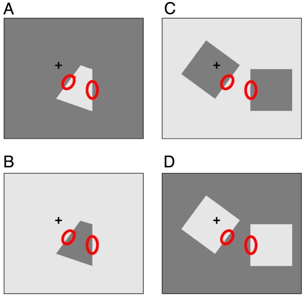
Example stimuli used. The two red circles in each condition represent the classical receptive fields (in the parafoveal region of the visual field) of the two neurons recorded while the animal fixates the cross. The two left panels show the “one-figure” conditions and the right panels the “two-figure” conditions. In each row, the two color contrast conditions are shown. Note that the stimulus within the classical receptive fields in the one-figure and two-figure conditions is identical for the same color contrast condition.

Procedure

Single-neuron activity was recorded extracellularly with Quartz-insulated Pt-W microelectrodes inserted through the dura mater. Areas V1 and V2 were identified by their retinotopic organization and by histological reconstruction of the recording sites, as described (Zhou et al., 2000). Action potentials were discriminated using a spike sorting device (Alpha Omega, Nazareth, Israel). Only isolated single unit activity was analyzed. Two electrodes 3 mm apart were lowered into the cortex. After isolating a cell on each electrode, we first characterized their selectivity (Zhou et al., 2000). Stationary bars were used to determine the color preference, and bars and drifting gratings to map the minimum response field of each cell. Orientation and disparity tunings were determined with moving bars. Subsequently, the binding test described above was performed. If the two cells had incompatible color selectivities, or if the receptive fields overlapped or had a spatial arrangement that precluded construction of the quadrilateral as described, we proceeded to isolate a new pair of cells. At least 13 complete responses (maximum 100, mean 45.6) for each stimulus condition were obtained from each pair of neurons. Only pairs in which each member produced at least 5 spikes/s mean firing rate in one of the four-border ownership/local contrast conditions were included because otherwise we felt that our stimuli were not appropriate to drive the cell.

The neurons started to respond with variable delays after stimulus onset. We found that reliable responses to the stimuli were obtained from all neurons after 60 ms. Many neurons in areas V1 and V2 are border-ownership selective, i.e., they respond differentially depending on which side of their receptive fields the perceptual foreground in the visual scene is located (Zhou et al., 2000). We characterized the border ownership property of each neuron by comparing the neuron responses when the figure was at opposite sides of the receptive field. The neuron’s border ownership selectivity B_s was defined as:

$$B_s=\frac{{\langle \sqrt{n_{\text{prefer}}^i+\frac{3}{8}}\rangle }_i-{\langle \sqrt{n_{\text{null}}^i+\frac{3}{8}}\rangle }_i}{{\sigma }_r},$$ (1)

where $n_{\text{prefer}}^i$ and $n_{\text{null}}^i$ are the neuron’s count of spikes for trial i during the interval [60 ms, 800 ms] in response to the preferred and the nonpreferred sides of figure in the receptive field, respectively. The bracket 〈〉_i denotes the average over all trials. The denominator σ_r is the square root of the residual variance calculated from a two-way ANOVA, in which the figure location (relative to the receptive field) is one factor and the local contrast polarity is the other factor. The ANOVA was performed on the squareroot transformed spike counts, $n^{\prime }=\sqrt{n+\frac{3}{8}}$. The transformation was used to stabilize the variance (Sachs, 1982). Border ownership selectivity is a property of individual neurons. To characterize border ownership selectivity for a pair of neurons, we define

$$B_p=B_{s1}\times B_{s2},$$ (2)

where B_s1, B_s2 are the border ownership selectivities computed from Equation 1 for the two individual neurons. B_p was not normally distributed, but inspection of quantile to quantile plots of various powers of B_p showed that the transformation using a power of 1/6 produced a normal distribution. We therefore used $B\frac{1}{p6}$ as the predictor for examining the correlation between synchronization and border ownership selectivity (Box & Cox, 1964).

Statistical measures and controls

Correlation functions

We divided time into bins of width 1 ms, each containing either 0 or 1 spike. This results in spike trains, $S_j^i\left(n\right)$, where n is the bin index, j is the number of the neuron, and i is the trial number. The spike train, $S_j^i\left(n\right)$, is a binary vector in which each component takes on either the value 0 if no spike is present in the interval [n, n + 1) ms in neuron j during trial i, or 1 if there is such a spike. Neurons typically responded to the stimuli with a fast transient response with a high, fast-changing instantaneous firing rate, followed by a period of sustained firing. We only analyzed the correlations during the sustained response period. To identify the latter, we fitted the function α + βexp(-kt) to the average peri-stimulus time histograms (PSTH; Figure 2, α = 23, β = 120, k = -0.019). The sustained response period was chosen to be the interval [160, 800] ms (right of vertical dashed line in the figure). We define a window function h(n) as h(n) = 1 if 160 ≤ n < 800 and h(n) = 0 otherwise.

Figure 2.

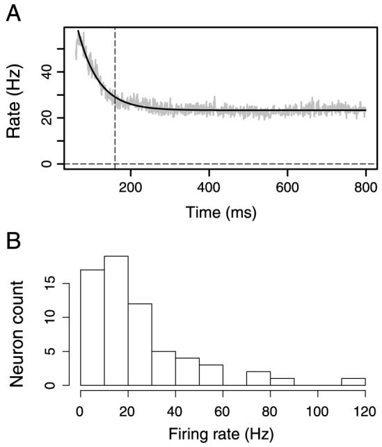
Neuronal firing rates. (A) The gray curve is the PSTH averaged over all 64 neurons. The PSTH is fitted with an exponential function plus a constant (black trace). Spike trains are analyzed in the interval from 160 ms to 800 ms, with the starting time marked by the dashed line. (B) Histogram of the mean firing rates (averaged over the interval [160 ms, 800 ms] after stimulus onset) in all stimulus conditions of all 64 analyzed neurons. The neuron with the highest firing rate (114 Hz) is a bursting neuron.

The cross-correlation function between two spike trains j, k for the ith trial is then calculated as

$$\begin{array}{cc}\hfill R_{j,k}^i\left(t\right)=& S_j^i\odot S_k^i\hfill \\ \hfill =& \sum _{\mu =160-w}^{799+w}{S}_j^i(\mu +t)S_k^i\left(\mu \right)h(\mu +t)h\left(\mu \right),\hfill \end{array}$$ (3)

where the first equality defines the cross-correlation operator ⊙ and t is the time shift between the two spike trains (-w ≤ t ≤ w). The parameter w is the window of the cross-correlation function (w = 100 ms in this study). Note that we omit the time argument in the ⊙ formulation here and everywhere below to alleviate notation. The cross-correlogram (see Figure 3A gray curve) of neurons j and k is the average of cross-correlation functions over all trials,

$$U_{j,k}\left(t\right)={\langle R_{j,k}^i\left(t\right)\rangle }_i,$$ (4)

where 〈〉_i again denotes the average across trials i.

Figure 3.

Example cross-correlation analysis. In this example, data of all the stimulus conditions are pooled together. (A) Gray curve, the cross-correlogram function; blue, the shift predictor; purple, the excitation covariogram. (B) auto-correlation function of the two neurons. The zero bin of the auto correlation function point exceeds the range shown and was not plotted. Gray, raw auto correlation function; blue, shift predictor; black, auto correlation function corrected for shift predictor. The dashed cyan lines mark the half integration width. (C) Calculation of the strength of synchrony. Black, ECC curve; green dotted lines are 2 standard deviations from the mean of the ECCs generated by randomization (see Materials and methods). The two cyan lines mark the integration interval for strength of synchrony. (D) Calculation of the strength of correlation. Black and green lines are as in C. The red line is the ECC smoothed with a Gaussian filter of standard deviation 10 ms. The middle cyan line marks the peak of the smoothed ECC. The other two cyan dashed line mark the integration width.

Shift predictor

We are interested in correlated activity of two neurons that is not due to covariation of their firing rates. For instance, small but systematic changes in the responses following stimulus onsets (even after removal of the large transients, see Figure 2 and accompanying discussion) may generate an excess of accidental coincidences. To correct for these and other stimulus-locked rate effects, we subtract the shift predictor (or “shuffle corrector,” see Figure 3A blue curve) from the cross correlogram. It is defined as the cross-correlation function of the PSTHs of the two neurons, i.e.

$${\langle S_j^i\rangle }_i\odot {\langle S_k^i\rangle }_i.$$ (5)

The shift-predictor corrected correlogram for neuron pair (j, k), referred to in the following as covariogram K_j,k, is thus

$$K_{j,k}\left(t\right)={\langle S_j^i\odot S_k^i\rangle }_i-{\langle S_j^i\rangle }_i\odot {\langle S_k^i\rangle }_i.$$ (6)

Excitability covariation

A possible source of spurious correlations are firing rates that covary in both neurons over periods of several trials, e.g., due to changing neuronal excitability (Brody, 1999; Roelfsema et al., 2004). We follow Roelfsema et al. (2004) to subtract the average spike counts from the neuron spike train for each trial. The average spike count per bin of neuron j during trial i is,

$$c_j^i=\frac{1}{640}\sum _{n=160}^{799}{S}_j^i\left(n\right).$$ (7)

The excitability covariation corrected covariogram function C_j,k(t) is computed as:

$$C_{j,k}\left(t\right)={\langle (S_j^i-c_j^i)\odot (S_k^i-c_k^i)\rangle }_i-{\langle S_j^i-c_j^i\rangle }_i\odot {\langle S_k^i-c_j^i\rangle }_i.$$ (8)

Defining the constants ${\beta }_j^i=\frac{c_j^i}{{\langle c_j^i\rangle }_i}$ and ${\beta }_k^i={\frac{c_k^i}{\langle c_k^i\rangle }}_i$, and the constant vectors B_j and B_k, each of whose component is ${\langle c_j^i\rangle }_i$ and ${\langle c_k^i\rangle }_i$, respectively, we can write Equation 8 as,

$$C_{j,k}\left(t\right)=K_{j,k}\left(t\right)-\mathrm{cov}({\beta }_j,{\beta }_k)B_j\odot B_k,$$ (9)

where the symbol cov(a, b) = 〈aⁱbⁱ〉_i - 〈aⁱ〉_i〈bⁱ〉_i denotes the covariance operation. The second term (see Figure 3A purple curve; note that this correction is usually very small) on the right hand side of Equation 9 is similar to the excitability covariogram proposed by Brody (1999), except that Brody used a more complicated neuronal model which includes a background term and a stimulus-induced term. However, since the background term is estimated from the activity recorded before the stimulus period, Brody’s correction usually does not converge to exactly 0 if we integrate the excitability covariation corrected covariogram from -∞ to ∞.

We will refer to the excitation corrected covariogram, Equation 9, as ECC in the following text.

Latency covariation

Another potential source of spurious correlations is latency covariation. As Brody (1999) has shown, if the responses of two neurons to a sensory stimulus shift together in time, a peak in their cross-correlation function around zero delay will result. We were concerned that such effects might contribute to the synchrony observed in our data. Let us assume for now that this were, in fact, the case. Then, by shifting the relative onset times of the two neurons in each trial appropriately it should be possible to remove the peak in the cross-correlation function. We therefore assigned time shifts that are common to both neurons, shifting spike data from trial i by t_i, and computed the ECCs C_j,k(t_i, t_i) as described (Equation 8), now based on time-shifted versions of the spike trains, $S_j^i(t-t_i)$, and $S_k^i(t-t_i)$. We then quantified the strength of the synchrony (as defined later in Significance tests of synchrony and correlation section), i.e., the weight of any potential peak in the cross-correlation function around zero time lag with half integral width 20 ms, and determined its statistical significance as described below (Significance tests of synchrony and correlation section). The correlation functions will depend on the choice of the time shifts. If the synchrony were, in fact, due to a set of time shifts of the spike trains, say by τ_i, then it will disappear for the choice t_i = -τ_i since this would exactly compensate for the time shift that caused synchrony and thus make it disappear.

We searched the space of all possible time shifts in the interval t_i ∈ [-10 ms, 10 ms] and used an optimization algorithm seeking to minimize the strength of synchrony with half integration width 50 ms. The minimization was performed by an exhaustive search for all time variables, first optimizing with respect to t₁, then t₂ etc., and repeating this procedure until the synchrony strength reached a minimum. As discussed above, if the peak were due to a common shift in latency, it would disappear for some set of time shifts (which in general would be different for each trial), namely the one that compensates for the latency shift common for both neurons. Before the minimization, there are 8 pairs significantly synchronized (the test method is described in Significance tests of synchrony and correlation section) in the one-figure condition and 3 pairs significant in the two-figure condition. The minimization procedure is likely to result in a loss of some significance since a large number of changes was applied (20 different time shifts for each trial, thus thousands of shifts for every neuron pair), each in the direction that decreased significance if possible. As expected, the statistical significance of synchrony was lost for some pairs but even after the minimization, 5 pairs remained significant in the one-figure condition and 2 pairs remained significant in the two-figure condition. No neuron pair changed significance in both binding conditions (note that the latency effect is independent of the binding condition). Note that this is a conservative method since we compare the significance of a minimized test statistic (the integral over the peak) against the distribution of nonminimized values. We did the same regression analysis on the shifted spike trains as discussed later, and our conclusions did not change. We therefore concluded that latency covariation effects can be ignored in our data.

Significance tests of synchrony and correlation

The ECC were averaged bin-wise over the two grayscale/color contrast conditions. Therefore, for each pair of neurons, two conditions—the one-figure and the two-figure condition—are considered in this study. To quantify the correlation between the ECCs of the two neurons, two measures were computed, “strength of synchrony” and “strength of correlation.”

Synchrony

The strength of synchrony $S_{j,k}^s$ measures the degree of synchronous firing. To compute it, we integrate the ECC of neurons j, k as defined in Equation 8, over the interval ±τ ms around 0 ms time lag (Figure 3C, the area under the black curve in the interval quantified by vertical cyan lines). In our discretized data set, this integral is the finite sum

$$\sum _{n=-\tau }^{\tau }{C}_{j,k}\left(n\right).$$ (10)

We can calculate the auto-correlogram function (Figure 3B gray curve, similar to Equation 4) and its shift predictor (Figure 3B blue curve) by the same equations shown in Correlation functions section and Shift predictor section, except the second neuron is identical to the first neuron. Then we can calculate the auto-covariogram function A_j (Figure 3B black curve) of neuron j as:

$$A_j={\langle S_j^i\odot S_j^i\rangle }_i-{\langle S_j^i\rangle }_i\odot {\langle S_j^i\rangle }_i.$$ (11)

The strength of synchrony $S_{j,k}^s\left(\tau \right)$ for neuron pair (j, k) is then defined as:

$$S_{j,k}^s=\frac{\sum _{n=-\tau }^{\tau }{C}_{j,k}\left(n\right)}{\sqrt{\sum _{n=-\tau }^{\tau }{A}_j\left(n\right)\sum _{n=-\tau }^{\tau }{A}_k\left(n\right)}},$$ (12)

,where τ is the half integration width for both ECC (Figure 3C marked by cyan dashed lines) and auto-correlogram (Figure 3B marked by cyan dashed lines). This definition¹ with auto-correlation normalization has the intuitively appealing property that S^s(τ) will approach Pearson’s cross-correlation coefficient of the two neurons trial-wise spike counts when τ → ∞ (Bair, Zohary, & Newsome, 2001; Roelfsema et al., 2004). In our case, S^s will approach 0 due to the excitability covariogram correction.

We use a permutation test (Efron & Tibshirani, 1993; Roy, Steinmetz, Hsiao, Johnson, & Niebur, 2007; Roy, Steinmetz, Johnson, & Niebur, 2000) to decide whether the observed peak is significantly different from what can be expected by chance, i.e., from computing the same quantity of strength of synchrony (Equation 12) from the ECC of spike trains of these two neurons that were not simultaneously recorded. We do this by generating 10000 permutations of pairs of trial indices (drawn without replacement) and number them with the index p = 1, 2, ..., 10000. Let ${\tilde{C}}_{j,k}^p$ be the ECC computed as in Equation 8 but using the pth permutation of the trial indices. The corresponding permuted strength of synchrony is

$${\tilde{Y}}_{j,k}^p\left(\tau \right)=\frac{\sum _{n=-\tau }^{\tau }{\tilde{C}}_{j,k}^p\left(n\right)}{\sqrt{\sum _{n=-\tau }^{\tau }{A}_j\left(n\right)\sum _{n=-\tau }^{\tau }{A}_k\left(n\right)}}.$$ (13)

The distribution given by the 10000 samples of ${\tilde{Y}}_{j,k}^p$ forms the null distribution. Given half integration width τ, we test the significance of the observed value for the integral around the peak, by using $S_{j,k}^s\left(\tau \right)$ from Equation 12 as the test statistic. If the value of $S_{j,k}^s\left(\tau \right)$ exceeds that of 95% of the values of ${\tilde{Y}}_{j,k}^p$ (at the p = 0.05 significance level), we will conclude that a significant peak is present in the ECC of neurons j and k, and the fraction of the distribution ${\tilde{Y}}_{j,k}^p$ with a value exceeding $S_{j,k}^s\left(\tau \right)$ is the p value of this test.

Correlation

The strength of correlation $S_{j,k}^c$ for neuron pair (j, k) is a more general measure used to quantify the correlations between the two neurons in the range of [-50, 50 ms], not necessarily at a time offset of zero. Such correlations would be manifested by peaks in the ECC. Let B₁₀() be a normalized Gaussian smoothing filter with standard deviation 10 ms around zero. The ECC is smoothed (Figure 3D blue curve) by convolving it with B₁₀, using the discrete convolution defined as,

$$B_{10}\otimes C_{j,k}\left(n\right)=\sum _{n^{\prime }=-\infty }^{\infty }{B}_{10}\left(n^{\prime }\right)C_{j,k}(n-n^{\prime }).$$ (14)

We then find the peak position (Figure 3D middle cyan line) T_peak of the smoothed ECC in the interval [-50, 50 ms]. Note that B₁₀ ⊗ C_j,k(T_peak) = max(B₁₀ ⊗ C_j,k(n)) where the max function always takes on the largest value of its argument for n ∈{-50, -49,..., 49, 50}. We thus obtain the strength of correlation for neuron pair (j, k),

$$S_{j,k}^c\left(\tau \right)=\frac{\sum _{n=-\tau +T_{\text{peak}}}^{\tau +T_{\text{peak}}}{C}_{j,k}\left(n\right)}{\sqrt{\sum _{n=-\tau }^{\tau }{A}_j\left(n\right)\sum _{n=-\tau }^{\tau }{A}_k\left(n\right)}}.$$ (15)

Here τ is the half integration width for both ECC (Figure 3D marked by two cyan dashed lines) and auto-correlogram. Comparing with Equation 12, correlation as defined here is equivalent to the strength of synchrony calculated around the peak of the ECC within the interval [-50, 50] ms rather than (always) around zero.

Our task is now to determine whether the strength of correlation found is higher than what can be expected by chance, under the null hypothesis that all trials are equivalent and that the simultaneously recorded activity is not more correlated than activity recorded in different trials. We applied a permutation test that is analogous to that previously introduced for the synchrony analysis. For 10000 permutations of the trial numbers, we compute the analog of Equation 14:

$$B_{10}\otimes {\tilde{C}}_{j,k}^p\left(n\right)=\sum _{n^{\prime }=-\infty }^{\infty }{B}_{10}\left(n^{\prime }\right){\tilde{C}}_{j,k}^p(n-n^{\prime }).$$ (16)

The peak of the pth permuted smoothed $\mathrm{ECC}(B_{10}\otimes {\tilde{C}}_{j,k}^p\left(n\right))$ is $T_{\text{peak}}^p$. Then given the half integration width τ, the pth permuted strength of correlation is ${\tilde{O}}_{j,k}^p\left(\tau \right)=\frac{{\sum }_{n=-\tau +T_{peak}^p}^{\tau +T_{peak}^p}{\tilde{C}}_{j,k}^p\left(n\right)}{\sqrt{{\sum }_{n=-\tau }^{\tau }{A}_j\left(n\right){\sum }_{n=-\tau }^{\tau }{A}_k\left(n\right)}}$.

The results of $O_{j,k}^p\left(\tau \right)$ form the null distribution for the permutation test. Completely analogous to the synchrony test, the test statistic to be used now is $S_{j,k}^c\left(\tau \right)$.

Bootstrap regression

For each of the neuron pairs recorded in the experiment, we estimate its intrinsic synchrony or correlation variability by the bootstrap method. For a pair of neurons (j, k) with spike trains $S_j^i$ and $S_k^i$, where i = 1, ..., N is the trial index and N is the number of trials, we generate “artificial experiments” by drawing randomly, with replacement, numbers i ∈[1, N] each of which corresponds to a trial index; thus, we draw a set of N pairs of spike trains. Let R^p be the vector of length N whose ith component is the ith number drawn, and p ∈[1, 10000] is the index in the set of trial indices. From this set of trial indices, we can find the geometrical mean firing rate F^p and compute the corresponding ECCs as in Equation 8, which we call ${\widehat{C}}_{j,k}^p$. We obtain for each of those the “bootstrapped strength of synchrony,” $B_{j,k}^p$

$$B_{j,k}^p\left(\tau \right)=\frac{\sum _{n=-\tau }^{\tau }{\tilde{C}}_{j,k}^p\left(n\right)}{\sqrt{\sum _{n=-\tau }^{\tau }{A}_j\left(n\right)\sum _{n=-\tau }^{\tau }{A}_k\left(n\right)}},$$ (17)

and “bootstrapped strength of correlation,” $R_{j,k}^p$

$$R_{j,k}^p\left(\tau \right)=\frac{\sum _{n=-\tau +T_{\text{peak}}}^{\tau +T_{\text{peak}}}{\tilde{C}}_{j,k}^p\left(n\right)}{\sqrt{\sum _{n=-\tau }^{\tau }{A}_j\left(n\right)\sum _{n=-\tau }^{\tau }{A}_k\left(n\right)}},$$ (18)

where T_peak was found from the smoothed ECC ${\widehat{C}}_{j,k}^p$ as described previously. The variability (noise) of synchrony and correlation can be estimated from the distribution of B^p and R^p.

To test whether the coefficient of the independent variables is significantly bigger than 0 or smaller than 0, we used a bootstrapped regression method (Kennedy & Gentle, 1980) with neuron intrinsic synchrony or correlation noise included in the regression. For example, we use strength of synchrony as dependent variable S_i and firing rate F_i and neuron pair BO selectivity B_i as independent variables, where i is the index of the data point. There are 32 (i = 1, ..., 32) data points corresponding to different neuron pairs. We draw, with replacement, 32 data points from the pool [F_i, B_i, S_i] and calculate the regression coefficient. Repeating this 10000 times, we obtain a distribution of the coefficients and we test the significance of the measured coefficient under the null hypothesis that there is no effect of the independent variable (coefficients are 0). To include the neuron’s intrinsic noise, we change the pool into [$F_i^p$, B_i, $S_i^p$], $R_i^p$, where $S_i^p$ is the “bootstrapped strength synchrony” defined above (Equation 17) and $F_i^p$ is the corresponding firing rate. When we draw the ith neuron data, we choose one (index p) of the bootstrapped synchrony $S_i^p$ and corresponding firing rate $R_i^p$ randomly. Then the distribution of the coefficients contains the neuronal intrinsic noise.

Timing of correlated events

The measures of correlation discussed so-far are concerned with the “heights” of the correlated peaks, i.e., how many correlated events occur. We were also interested in the timing of these events, i.e., at what times relative to synchrony the peaks occur. We searched for peaks in the full range [-99, 99] ms that is available with our choice of the window w = 100 ms (see Equation 3). In our parameterization, peak positions are integers ∈ [0, 99] corresponding to the position of the peaks in the strength of correlation (positive and negative integers are pooled since the sign only reflects the arbitrary ordering of neurons). The histogram of the peak positions (64 peaks in total, Figure 8) for both figure conditions was plotted in 5 bins, each 20 ms wide.

Figure 8.

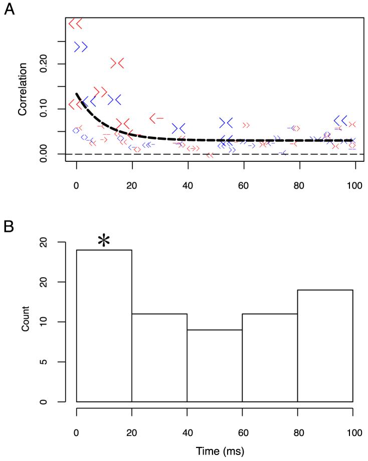
Peak position distributions. (A) Correlation strengths versus peak positions for one-figure condition (red symbols) and two-figure condition (blue symbols). The symbols 〉, 〈 indicate the preferred border ownership neuron direction, and - indicates that the neuron is not border ownership selective (less than 0.2 in border ownership selectivity). Significant strength of correlation was marked by large symbols. All 64 data points are fitted with an exponential function plus a constant elevation (black thick line). (B) Histogram of peak position distributions for the two binding conditions. The first bin is significantly higher than expected by chance by binomial test (method Significance tests of synchrony and correlation section).

Is there a significant number of counts in one bin? We proceed to answer this question as follows. The null hypothesis is that peak positions are uniformly distributed in the possible 100 positions {0, 1, ..., 99}. Thus, the number of counts k in one bin of a histogram under the null hypothesis is a random number following the binomial distribution, namely the probability of k counts is $\left(\begin{array}{c}\hfill 64\hfill \\ \hfill k\hfill \end{array}\right){\left(\frac{1}{5}\right)}^k{(1-\frac{1}{5})}^{64-k}$. The p value under the null hypothesis would be the probability (or p value) that the number of the counts in one bin larger than the observed count o:

$$\sum _{j=0}^{64}\left(\begin{array}{c}\hfill 64\hfill \\ \hfill k\hfill \end{array}\right){\left(\frac{1}{5}\right)}^k{\left(1-\frac{1}{5}\right)}^{64-k}.$$ (19)

Results

Firing rates and coincidence rates

Data from 32 pairs of neurons met the criteria (see Procedure section) for analysis in this study. Of the neurons comprising these pairs, 9 were from area V1, 52 from area V2, and 3 from near the V1-V2 border and difficult to assign unambiguously to either area. The neurons formed 3 V1-V1 pairs, 4 V1-V2 pairs, 3 V2-ambiguous pairs, and 22 V2-V2 pairs. We performed linear regression with a 2-level categorical independent variable to describe the neuron pair composition. The first level composed the 22 V2-V2 neuron and the second level the ten other pairs. Using this independent variable in the linear model to explain synchrony and correlation effects with the other independent variables (rate, border ownership, binding), we found that the neuron pair composition variable coefficient did not show a significant effect (p = 0.05). Therefore, results from the 32 pairs were pooled.

We first quantified the mean firing rates of the 64 analyzed neurons over the sustained period, 160-800 ms. Their firing rates, averaged over all stimulus conditions, varied broadly as shown in Figure 2B. This distribution has a mean of 23.8 Hz, a median of 17.8 Hz, and its mode is close to 15 Hz. There were 7 neurons whose average firing rates were lower than 5 Hz; note that this does not contradict the neuron screening rule (Procedure section) because their firing rate in the optimal stimulus condition was higher than 5 Hz.

To provide a first, albeit rough, idea of the prevalence of correlated firing in the population, we computed a simple measure of synchrony, the mean ratio of coincidences/spike averaged over all neurons during the period of sustained firing (160 to 800 ms, see Figure 2). We defined a coincidence here as an event in which the two neurons fire within ±2 ms and we found an average of 0.12 coincidences/spike for both the one-figure condition (median 0.085) and for the two-figure condition (median 0.082). There was no significant difference of the coincidence rate for these 64 neurons between the stimulus conditions (paired t test, p = 0.397). These numbers are also close to what would be expected from independently firing neurons: given that their mean firing rate is 23.8 spikes/s (see Figure 2), an average of 23.8/1000 × 5 = 0.119 spikes in one neuron occur by chance within a ±2 ms window relative to a spike in the other neuron. By this simple measure, the neurons are therefore only weakly correlated.

Synchrony is independent of binding condition

We corrected for the influence of various firing rates and defined strength of synchrony and correlation based on a method suggested by Roelfsema et al. (2004). It has the property that the strengths of synchrony and correlation will approach zero if the integration width is the whole cross-correlation window length (see Figure 4). Usually, the strength of synchrony or correlation first reaches a peak and with increasing integration width it decays to zero. The strength at the peak position is the best estimation of the short term correlation coefficient, beyond that the strength will include more and more noise contributions (Bair et al., 2001). From Figure 4, we find a peak position for the averaged strength of synchrony at 34 ms, and 18 ms for the average strength of correlation.

Figure 4.

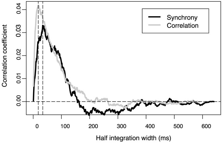
Averaged synchrony (black curve) and strength of correlation (gray curve) over all the stimulus conditions and all the neuron pairs. The dotted vertical lines mark the peak position for the strength of correlation (18 ms) and strength of synchrony (34 ms).

In the one-figure condition, the two neurons represent two edges that are part of the same object. According to the BBS hypothesis (e.g., Singer, 1993, 1999), the activity of these neurons should be synchronized. On the other hand, in the two-figure condition, the two neurons represent parts of two different objects and, according to the BBS hypothesis, they should not be synchronized.

We applied randomization tests to the whole population of 32 pairs of neurons for their strength of synchrony (normalized integral of the ECC around 0 ms time lag), S^s(34), and correlation strength (normalized integral of the ECC around peak of the ECC), S^c(18), i.e., at their respective peaks shown in Figure 4. For strength of synchrony, we found that 5 pairs were significant in the one-figure condition only, 4 pairs were significant in both binding conditions (one-figure and two-figure conditions), and no neuron pair was significant in the two-figure condition only. For strength of correlation, 3 pairs were significant in the one-figure condition only, 4 pairs were significant in both binding conditions, and 3 pairs were significant in the two-figure condition. In the one-figure condition, both S^c(18) and S^s(34) were significant in 6 pairs of the neurons, while in the two-figure condition, both S^c(18) and S^s(34) were significant in 4 pairs of the neurons, as a result of the tendency of the peaks in the ECCs to be centered around 0 ms time lag.

It has been shown that the strength of synchrony covaries with the geometrical mean of the neuron pair firing rates (de la Rocha et al., 2007). To test whether there is a difference between one-figure and two-figure conditions, we performed a linear regression with S^s(34) as the dependent variable and binding condition and the firing rate of a neuron pair (defined as the geometrical mean of the firing rates of the two neurons) as independent variables, plus one random intercept term which quantifies the neuron identity effects. We found a significant firing rate dependence (p = 0.0003), but the effects of binding condition (p = 0.661) and the interaction between rate and binding condition (p = 0.088) were not significant. Thus, after removing the firing rate effects, the effect of the binding condition disappeared. Applying the same model to the strength of correlation S^c(18), we obtain a similar result. There was a significant firing rate effect (p = 0.0335), but the effects of binding condition (p = 0.735) and interaction (p = 0.401) were not significant.

To maximize the signal to noise ratio, we chose to use the integration intervals that produced maximum strength of synchrony or correlation in the averaged strength curve in Figure 4. To what extent do the results depend on this choice? Using the same linear model, we examined a range of integration windows ±10 ms around the maxima, i.e., [24, 44] ms for strength of synchrony and [8, 28] ms for strength of correlation. The p values,² summarized in Figure 5, confirm that, for the whole range of integration widths, synchrony and correlation significantly depend on the neuron pair firing rate but not on the binding conditions.

Figure 5.

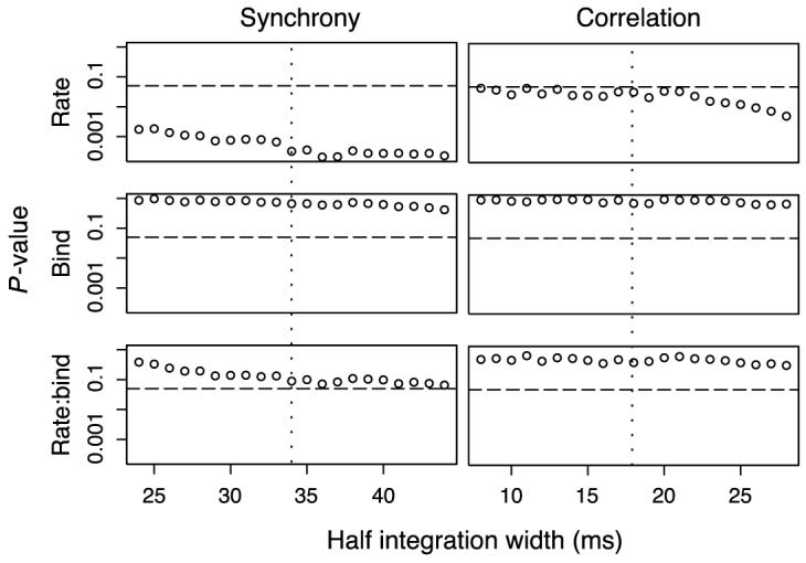
Linear model for the dependence of synchrony and correlation of a neuron pair on its firing rate and binding condition. The model is described in the text (Synchrony is independent of binding condition section), the dependent variables are synchrony S^s(τ), τ = 24, ..., 44 (left column) and correlation S^c(τ), τ = 8, ..., 28 (right column), respectively. Shown is the dependence of the p values on the half integration width. The horizontal line is 0.05, i.e., p values below this line are considered significant at the p = 0.05 level. The vertical dotted line marks the peak of the half integration width in the averaged synchrony (left) or correlation strength (right), as shown in Figure 4. Neither synchrony nor correlation depended on the binding condition but both depend on rate for all integration widths.

We conclude that we do not find support for the binding by synchrony hypothesis when firing rate effects are taken into account. The strength of synchrony or correlation significantly depended on the firing rate of the neuron pairs (defined as the geometrical mean of the two rates). One possible explanation of this dependence is the nonlinearity of the neuronal input-output function (de la Rocha et al., 2007).

Dependence of synchrony and correlation on border ownership selectivity

Following our previous studies (Zhou et al., 2000), we assumed that information about the figure geometry is carried by border-ownership selective neurons. Based on our model of BO coding (Craft, Schütze, Niebur, & von der Heydt, 2007), we hypothesized that spike trains of neurons that are widely separated in cortex should be correlated only if the neurons are BO selective. Thus, we tested if synchrony or correlation depended on the neuron pair border ownership selectivity of the neuron pairs. We therefore expanded the linear regression model discussed in the previous section by adding dependence on neuron pair BO selectivity. As shown in Table 1, both S^s(34) and S^c(18) significantly depended on neuron pair BO selectivity and, furthermore, strength of both synchrony and correlation increased with the BO selectivity (coefficients are positive). Firing rate was found significant in the strength of synchrony and close to significant (p = 0.076) in the strength of correlation. We did not find evidence of binding nor any significant interaction effects for either synchrony nor correlation.

Table 1.

Linear mixed model for strength of synchrony S^s(34) and correlation S^c(18) in terms of neuron pair effect (a random variable in the intercept of the model), geometrical mean of the neuron pair firing rates (rate, a continuous variable), the neuron pair border ownership selectivity effect (bos, a continuous variable), the stimulus binding effect (bind, a categorical variable, 0 is one-figure condition and 1 is two-figure condition), and the three interaction effects. The coefficients and the corresponding p values of the test that the respective coefficient is different from zero (t test) are listed for synchrony and correlation

	Synchrony		Correlation
Terms	Coefficient	p value	Coefficient	p value
Intercept	-0.169	0.0172	-0.114	0.044
Rate	5.846	0.0388	4.048	0.076
Bos	0.152	0.0467	0.151	0.017
Bind	0.043	0.3270	0.040	0.287
Rate:bos	-2.082	0.4473	-2.433	0.287
Rate:bind	-1.713	0.1143	-0.671	0.463
Bos:bind	-0.043	0.3952	-0.043	0.324

Again, we examined how these results depended on the integration width. The p values for the same linear model as discussed in the previous paragraph are summarized in Figure 6. Both synchrony and correlation depended significantly on BO selectivity for a range around the integration widths around 34 ms for synchrony and 18 ms for correlation, although significance is only marginal for the former. The effect of rate is only significant for the strength of synchrony, and correlation was found to be close to significant for some smaller choices of the integration width. Importantly, the binding condition did not have a significant effect, nor did any of the interactions.

Figure 6.

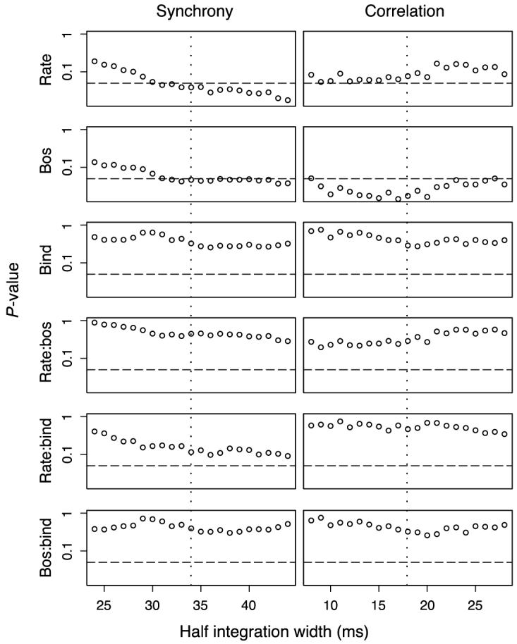
Same as Figure 5 except that neuron pair BO selectivity was added as an independent variable. The results of the model for the preferred integration width are summarized in Table 1. Both synchrony and correlation depend on the neuron pair BO selectivity.

Considering neuronal intrinsic noise (estimated by the bootstrap method, see method Bootstrap regression section), we performed a bootstrapped regression with the same linear model. The coefficients of none of the independent variables were significant.³ The loss of statistical power was expected, because of the limited number of only 32 neuron pairs (the power of the bootstrap regression is limited by the number of data points) and because the bootstrapping procedure contributes additional “noise.” The evidence of a dependence on firing rate and neuron pair BO selectivity is thus weaker in these results than in the linear regression model. Nevertheless, the results of this test still convey the same message that there is little support for the BBS hypothesis.

Synchrony is independent of the directional selectivity of border ownership neuron

We have shown in the previous sections that the two different stimulus geometries make no difference for the synchrony or correlation strengths, which, however, depended significantly on the neuron pair BO selectivity (though not in the bootstrapped test in Dependence of synchrony and correlation on border ownership selectivity section). This suggested that border ownership selective neurons receive common inputs. In addition to their preferred edge orientation, border ownership neurons have a preferred direction for the side of figure, which we have, so far, ignored.⁴ We examined whether the strength of synchrony or correlation also depends on the directional selectivity. We selected border ownership selective neuron pairs if the border ownership selectivity was stronger than 0.2 for both of the neurons, resulting in 22 pairs with this property. This group was divided into 3 sub-groups: the 〉〈 group (5 pairs), in which the preferred sides of border ownership pointed towards each other; the 〈〉 group (4 pairs), in which the preferred sides of border ownership pointed away from each other; and the ≪ group (13 pairs), in which the preferred sides pointed in the same direction. Including this 3-level categorical variable in the analysis, we tested a new linear model by analysis of variance. Note that the neuron pair BO selectivity was eliminated as a dependent variable since only BO selective neurons were included in this analysis. The p values are summarized in Figure 7. We found no evidence for a directional selectivity effect. Significance was only reached by rate. Again, we found no support of the BBS hypothesis.

Figure 7.

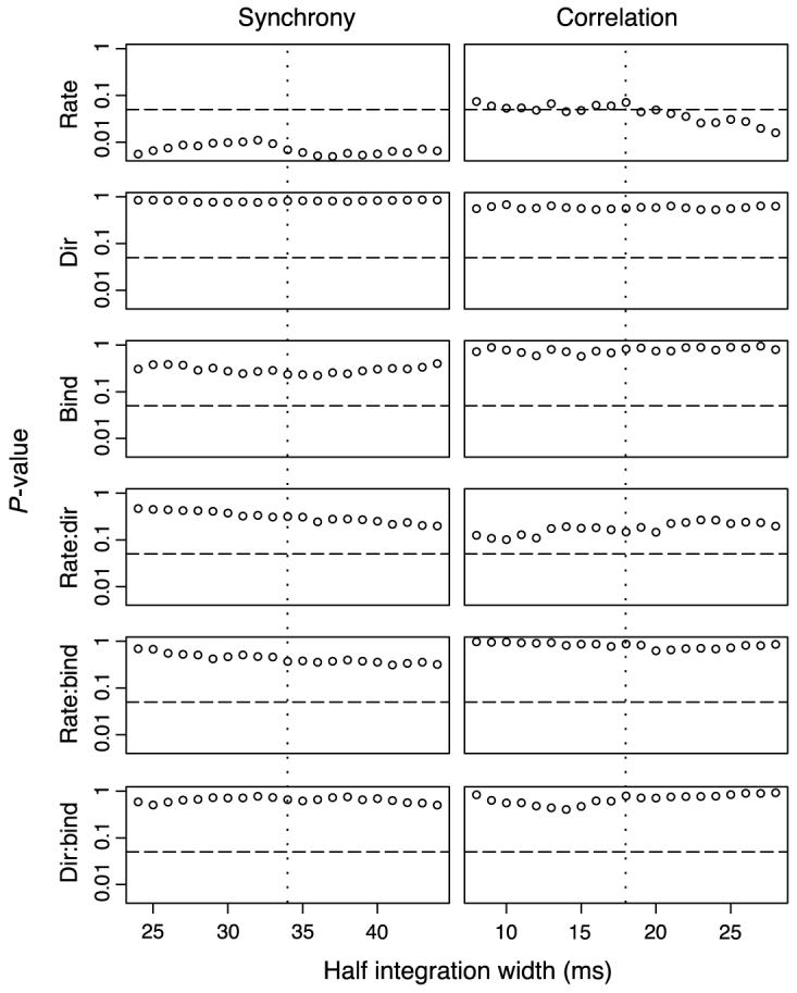
Same as Figure 6 except that only the 22 neuronal pairs are included in which both neurons are BO selective. Strength of synchrony or correlation is explained by geometrical mean firing rates (rate, a continuous variable), directional selectivity (dir, a 3-level categorical variable indicating 〉〈, 〈〉 and ≪ neuron pairs; see text for explanation), stimulus binding effect (bind, a categorical variable, 0 is one-figure condition and 1 is two-figure condition) and their interactions, and the neuron pair effect (a random variable in the intercept of the model). The p values are calculated from analysis of variance of this linear model. Neither the synchrony nor the correlation depended on the directional selectivity.

Peak positions

So far, we have distinguished only between correlation with peaks close to zero, referred to as synchrony, and correlation at time lags in the window ±50 ms, and we have only studied whether any such correlation occurred, irrespective of time lag. We will now examine at which time lag the correlated activity occurred. We expanded the search range for the peak positions to ±99 ms. The peak positions of the strength of correlations S^c(18) are summarized in Figure 8A. The peaks cover the whole [0 ms, 99 ms] range. However, for neuron pairs with significant strength of correlations (by randomization test p < 0.05, large symbols in Figure 8A), the lags are mostly contained within the interval [0, 20] ms. Peaks for neuron pairs with smaller strength of correlations are spread more widely and their peak positions may be due to random effects. We fitted the strength of correlation vs. peak position data with an exponential plus constant (αexp(βx) + c) and found α, β, and c (α = 0.104, β = -0.105, c = 0.0303) to be all significantly different from zero (p < 0.05, t test). In the peak histogram (Figure 8B), the first bin was significantly higher than expected by chance (p = 0.042 binomial test), the other bins were not significant. Thus, we conclude that peaks in the correlation function are mostly found in the [0, 20 ms] interval.

Discussion

In the present work, we tested the binding-by-synchrony hypothesis by studying neural activity in striate and (primarily) extrastriate cortex of awake behaving monkeys. While spiking activity of pairs of neurons in area V2 (as well as of some V1 neurons) was recorded, the animal saw either one or two visual objects. Importantly, the stimulus geometry was carefully adjusted such that the receptive fields of the two neurons whose activity was recorded received identical visual input in both cases. Thus, whether one or two visual objects were present could not be decided from the visual input to these receptive fields. The BBS hypothesis predicts that spiking activity of these two neurons should be more correlated when the visual inputs to their receptive fields are part of one object, compared to when they represent parts of two objects.

There are many studies on synchrony, but few if any have tested the feature binding paradigm as directly as we did in the experiments described here. More typically, the “binding” conditions were either a single bar or two aligned bars moving in synchrony (Gray, Engel, König, & Singer, 1990; Kreiter & Singer, 1992) or plaids of two gratings (Engel, König, & Singer, 1991b; Thiele & Stoner, 2003). A recent study by Palanca and DeAngelis (2005) in primate area MT used a type of visual stimuli similar to ours but no single unit data were recorded (only multi-unit activity and local field potentials). For the stimulus corresponding to our 1-figure condition, significantly stronger synchrony was obtained than in the 2-figure condition in the LFP and some of the MUA data but the synchrony was considered weak.

We found that the average number of spikes recorded from one of the neurons that were synchronous with spikes in the other, simultaneously recorded neuron, was close to what is expected for independently firing neurons, and by this measure the observed synchrony can be considered weak. It is remarkable, however, that a substantial fraction of our neuron pairs (9 out of 32) showed statistically significant synchrony in one or both of the stimulus conditions, even though our cells pairs were recorded on two electrodes separated by 3 mm, a relatively large distance in cortex. Previous studies have shown that the probability of finding correlation decreases sharply with distance (Hata, Tsumoto, Sato, & Tamura, 1991). Thus, the frequency of synchronizing pairs in our study is notable. It also demonstrates the sensitivity of our methods for detecting even small levels of synchrony.

Another reason to emphasize the substantial distance between the electrodes is that our analysis required that the receptive fields were well separated. Previous studies that analyzed synchronous oscillations have often studied neurons with overlapping receptive fields or were limited to neurons of similar preferred orientation and aligned receptive fields (e.g., Castelo-Branco, Goebel, Neuenschwander, & Singer, 2000; Engel, König, Kreiter, & Singer, 1991a; Engel et al., 1991b).

While our rough measure of coincidences/spike showed that synchronous events occurred in both the binding and nonbinding condition, there was no significant difference between the rate of events in the two conditions. We therefore applied a more controlled test of the significance of the observed strength of synchrony and correlation, using integration widths that maximize these quantities over the whole population (Figure 4). The most important question is whether synchrony and/or correlation vary with the binding condition, i.e., between the one-figure and two-figure conditions. Since correlation between spike trains is known to depend on firing rate, we used a linear model with rate and binding condition as independent variables (rate: continuous, binding condition: categorical). For both synchrony and correlation, we found a significant rate dependence but no dependence on the binding condition nor on the interaction between these two variables. We further showed that these results do not depend on the choice of the integration window (Figure 5). These results are not consistent with predictions of the BBS hypothesis.

A more differentiated view emerged when we took into account another component of perceptual organization. It was observed long ago by Gestalt psychologists that the human visual system segregates displays into foreground and background regions and assigns borders between regions to the foreground (Rubin, 1921). We have recently shown that this property of border ownership is represented in the activity of individual neurons in the monkey visual cortex, especially the secondary visual area V2 (Qiu, Sugihara, & von der Heydt, 2007; Qiu & von der Heydt, 2005, 2007; Zhou et al., 2000). A substantial fraction of neurons in this area were not only orientation tuned but also selective for the figure-ground assignment of the stimulus in their receptive field. These neurons modify their firing rates dependent on whether a contour presented in their receptive field belongs to an object on their preferred foreground side or to an object on the opposite side (“border ownership coding”). Note that this observation neither supports nor contradicts the BBS hypothesis (border ownership coding is a property of the firing rates of individual neurons, not the correlation between spike trains of pairs of neurons) and both mechanisms could very well coexist and interact with each other. It is thus natural to study the relationship between these two mechanisms.

In the next phase of our study, we therefore studied how synchrony and correlation are influenced by the binding condition and the strength of border ownership selectivity. We found that synchrony between two neurons depended on their mean rate as well as on the strength of their combined border ownership signal. There was also a significant effect of border ownership strength (but not of rate) on the correlation. Significance was not reached for any effect in a bootstrapped version of the same test (known to have less statistical power). The most important conclusion from both tests is that we found again no effect of the binding condition on either synchrony or correlation, and this result was valid for a whole range of integration windows (Figure 6).

The dependence of synchronization on border ownership strength of the pair rises a new question: are all the border ownership neurons synchronized similarly, or are there subgroups of the border ownership neurons which synchronize to different levels. In order to test this, we continued our examination including only pairs of border ownership neurons, and divided them in three direction categories depending on their side of figure preference: parallel, in and out. Since this sample includes only the border ownership selective neurons, we replaced the border ownership strength with the direction categories as an independent variable. We again found a significant dependence of synchronization on rate and no dependence on the binding condition. However, we did not find a significant dependence of synchrony or correlation on the direction category.

To characterize the correlation structure of the spike-trains in more detail, we describe in Peak positions section the locations of peak positions. We find a wide distribution over the whole range considered, 0 to 99 milli-seconds, but the peaks of neuron pairs with significant strength are concentrated closer to zero (synchrony), in the first bin, [0, 20 ms].

How can our findings be understood in the context of the binding by synchrony hypothesis? The prediction of the BBS hypothesis is that all neurons involved in representing a visual object should synchronize, and that all neurons that represent different objects should not be synchronized. We found no evidence for this prediction to be true. Strength of synchrony (and correlation) depended on several factors, most robustly mean firing rate of the two neurons of a pair, but in no case was the binding condition found to be one of the factors.

How can our findings then be understood from a more general point of view? Our results show that the fact that the input to two neurons is from one visual object by itself does not make their firing more correlated than if the input results from two objects. However, the tendency to synchronize increases with the degree of border ownership selectivity of a pair (that is, the product of their border ownership selectivities). Border ownership selectivity requires integration of the image context far beyond the classical receptive field (Qiu & von der Heydt, 2005; Zhou et al., 2000). Thus, we interpret the higher tendency of border ownership selective pairs to synchronize as a consequence of their participation in circuits of image context integration. Studies of V1 have shown that synchrony and correlation occur frequently between cells at a distance of a few hundred microns from each other but rarely between cells that are more widely separated (Hata et al., 1991; Kohn & Smith, 2005; Samonds, Zhou, Bernard, & Bonds, 2006). This is consistent with anatomical studies showing that horizontal fibers in the cortex extend only a few millimeters (Lund, Angelucci, & Bressloff, 2003). As we have pointed out (Craft et al., 2007), the range and speed of image context integration found in border ownership coding cannot be explained by connectivity over such short distances but is likely to involve feedback from another, higher-level, area. The feedback connections fan out widely and consist of fast-conducting white matter fibers. Our model (Craft et al., 2007) explains border ownership selectivity by a relatively simple mechanism in which grouping cells (at some higher level, e.g., V4) sum edge signals of V2 in cocircular arrangement, and, via feedback, modulate the activity of the corresponding V2 cells. Each of the figures in the present study would activate a grouping cell (or a small cluster of such cells) which, by feedback, would enhance the activity of the V2 cells representing the contour of the figure. Because each grouping cell reaches most of the V2 cells in the representation if the figure, it is likely to generate synchrony in these cells, and this, we argue, is the synchrony and correlation that our analysis detected in the present study. Limitations inherent in the nature of both the experimental data set (mainly the relatively small number of neuronal pairs recorded) and the modeling paradigm (the model described in Craft et al., 2007, is based on mean firing rates and cannot make detailed predictions about correlations between spikes) prevent us from reaching a stronger conclusion on the origin of this synchronization.

An important result of our study is that neurons fail to show significant synchrony in the binding condition despite the fact that the majority of these neurons signal border ownership by their firing rate. The assignment of border ownership is a form of feature binding. The four sides of a square, for example, are assigned to the same region. In our model (Craft et al., 2007), this binding is explicitly represented by the activity of the grouping cells: activation of a grouping cell enhances the signals representing the four edges that make up the square. We have recently shown that border ownership selective V2 neurons are also modulated by volitional (top-down) attention, and that this modulation is specific for the side of border ownership preference, indicating that selective attention mechanisms use the same grouping circuits that generate border ownership selectivity (Qiu & von der Heydt, 2007). This finding is direct evidence that border ownership coding is feature binding: attention to a figure produces selective enhancement of the edge signals assigned to that figure. Thus, the border ownership circuits serve as a binding mechanism, enabling object-based attention. In this mechanism binding is represented by firing rate, and synchrony, as we have explained above, is a byproduct of this mechanism.

Of course, this does not mean that synchrony is not used downstream in the processing hierarchy in addition to the enhancement of firing rate. Indeed, it is plausible in principle that nature would make use of a strong and easily identifiable feature like synchronous firing for some purposes. Specifically, synchronous firing could be used to distinguish attended from unattended stimuli (Niebur & Koch, 1994; Niebur, Koch, & Rosin, 1993). Experimental evidence for this hypothesis is accumulating (Fries, Reynolds, Rorie, & Desimone, 2001; Steinmetz et al., 2000). These studies indicate that the system uses synchrony for “top-down” attention, but our results make it seem unlikely that synchrony plays a role in feature binding.

Several limitations of our study are noted. The first is the relatively small number of neuron pairs. We found it difficult with the quartz-fiber electrodes to isolate and hold two cells long enough in an awake animal to map their receptive fields and characterize their selectivities and then record a sufficient number of spikes in both of them for the present analysis. Thus, the yield of these experiments was low.

A limitation of our study is also the use of a behavioral task that engaged attention at the fixation target. This task was deliberately chosen because our goal was to study binding and separate the influence of binding from that of attention. In neurophysiological experiments, we found that border ownership coding occurs simultaneously and in parallel for multiple figure displays, and, although most border ownership selective neurons are also influenced by top-down attention, the border ownership signal is generated independently of attention (Qiu & von der Heydt, 2007). Future work will elucidate how more complex behavioral tasks, like those involving selective attention to stimuli in the receptive fields of the neurons studied, as well as short-term memory, influence neuronal spike trains in V2 and their correlation structures.

References

- Bair W, Zohary E, Newsome WT. Correlated firing in macaque visual area MT: Time scales and relationship to behavior. Journal of Neuroscience. 2001;21:1676–1697. doi: 10.1523/JNEUROSCI.21-05-01676.2001. [DOI] [PMC free article] [PubMed] [Google Scholar]
- Bernander O, Koch C. The effect of synchronized inputs at the single neuron level. Neural Computation. 1994;6:622–641. [Google Scholar]
- Box GEP, Cox DR. An analysis of transformations. Journal of the Royal Statistical Society Series B. 1964;26:211–246. [Google Scholar]
- Brody Disambiguating different covariation types. Neural Computation. 1999;11:1527–1535. doi: 10.1162/089976699300016124. [DOI] [PubMed] [Google Scholar]
- Castelo-Branco M, Goebel R, Neuenschwander S, Singer W. Neural synchrony correlates with surface segregation rules. Nature. 2000;405:685–689. doi: 10.1038/35015079. [DOI] [PubMed] [Google Scholar]
- Craft E, Schütze H, Niebur E, von der Heydt R. A neural model of figure-ground organization. Journal of Neurophysiology. 2007;97:4310–4326. doi: 10.1152/jn.00203.2007. [DOI] [PubMed] [Google Scholar]
- de la Rocha J, Doiron B, Shea-Brown E, Josic K, Reyes A. Correlation between neural spike trains increases with firing ratee. Nature. 2007;448:802–806. doi: 10.1038/nature06028. [DOI] [PubMed] [Google Scholar]
- de Oliveira SC, Thiele A, Hoffmann KP. Synchronization of neuronal activity during stimulus expectation in a direction discrimination task. Journal of Neuroscience. 1997;17:9248–9260. doi: 10.1523/JNEUROSCI.17-23-09248.1997. [DOI] [PMC free article] [PubMed] [Google Scholar]
- Eckhorn R, Bauer R, Jordan W, Brosch M, Kruse W, Munk M, et al. Coherent oscillations: A mechanism of feature linking in the visual cortex? Multiple electrode and correlation analyses in the cat. Biological Cybernetics. 1988;60:121–130. doi: 10.1007/BF00202899. [DOI] [PubMed] [Google Scholar]
- Efron B, Tibshirani RJ. An introduction to the bootstrap. Chapman & Hall; New York: 1993. [Google Scholar]
- Engel AK, König P, Kreiter AK, Singer W. Synchronization of oscillatory neuronal responses between striate and extrastriate visual cortical areas of the cat. Proceedings of the National Academy of Sciences of the United States of America. 1991a;88:6048–6052. doi: 10.1073/pnas.88.14.6048. [DOI] [PMC free article] [PubMed] [Google Scholar]
- Engel AK, König P, Singer W. Direct physiological evidence for scene segmentation by temporal coding. Proceedings of the National Academy of Sciences of the United States of America. 1991b;88:9136–9140. doi: 10.1073/pnas.88.20.9136. [DOI] [PMC free article] [PubMed] [Google Scholar]
- Fries P, Reynolds JH, Rorie AE, Desimone R. Modulation of oscillatory neuronal synchronization by selective visual attention. Science. 2001;291:1560–1563. doi: 10.1126/science.1055465. [DOI] [PubMed] [Google Scholar]
- Gray C, Engel A, König P, Singer W. Stimulus-dependent neuronal oscillations in cat visual cortex: Receptive field properties and feature dependence. European Journal of Neuroscience. 1990;2:607–619. doi: 10.1111/j.1460-9568.1990.tb00450.x. [DOI] [PubMed] [Google Scholar]
- Gray C, Singer W. Stimulus-specific neuronal oscillations in orientation columns of cat visual cortex. Proceedings of the National Academy of Sciences of the United States of America. 1989;86:1698–1702. doi: 10.1073/pnas.86.5.1698. [DOI] [PMC free article] [PubMed] [Google Scholar]
- Hata Y, Tsumoto T, Sato H, Tamura H. Horizontal interactions between visual cortical neurones studied by cross-correlation analysis in the cat. Journal of Physiology. 1991;441:593–614. doi: 10.1113/jphysiol.1991.sp018769. [DOI] [PMC free article] [PubMed] [Google Scholar]
- Kennedy WJJ, Gentle JE. Statistical computing. Marcel Dekker; New York: 1980. [Google Scholar]
- Kohn A, Smith MA. Stimulus dependence of neuronal correlation in primary visual cortex of the macaque. Journal of Neuroscience. 2005;25:3661–3673. doi: 10.1523/JNEUROSCI.5106-04.2005. [DOI] [PMC free article] [PubMed] [Google Scholar]
- Kreiter AK, Singer W. Oscillatory neuronal responses in the visual cortex of the awake macaque monkey. European Journal of Neuroscience. 1992;4:369–375. doi: 10.1111/j.1460-9568.1992.tb00884.x. [DOI] [PubMed] [Google Scholar]
- Lund JS, Angelucci A, Bressloff PC. Anatomical substrates for functional columns in macaque monkey primary visual cortex. Cerebral Cortex. 2003;13:15–24. doi: 10.1093/cercor/13.1.15. [DOI] [PubMed] [Google Scholar]
- Mikula S, Niebur E. Rate and synchrony in feedforward networks of coincidence detectors: Analytical solution. Neural Computation. 2005;14:881–902. doi: 10.1162/0899766053429408. [DOI] [PMC free article] [PubMed] [Google Scholar]
- Niebur E, Koch C. A model for the neuronal implementation of selective visual attention based on temporal correlation among neurons. Journal of Computational Neuroscience. 1994;1:141–158. doi: 10.1007/BF00962722. [DOI] [PubMed] [Google Scholar]
- Niebur E, Koch C, Rosin C. An oscillation-based model for the neural basis of attention. Vision Research. 1993;33:2789–2802. doi: 10.1016/0042-6989(93)90236-p. [DOI] [PubMed] [Google Scholar]
- Palanca BJA, DeAngelis GC. Does neuronal synchrony underlie visual feature grouping? Neuron. 2005;46:333–346. doi: 10.1016/j.neuron.2005.03.002. [DOI] [PubMed] [Google Scholar]
- Qiu FT, Sugihara T, von der Heydt R. Figure-ground mechanisms provide structure for selective attention. Nature Neuroscience. 2007;10:1492–1499. doi: 10.1038/nn1989. [DOI] [PMC free article] [PubMed] [Google Scholar]
- Qiu FT, von der Heydt R. Figure and ground in the visual cortex: V2 combines stereoscopic cues with Gestalt rules. Neuron. 2005;47:155–166. doi: 10.1016/j.neuron.2005.05.028. [DOI] [PMC free article] [PubMed] [Google Scholar]
- Qiu FT, von der Heydt R. Neural representation of transparent overlay. Nature Neuroscience. 2007;10:283–284. doi: 10.1038/nn1853. [DOI] [PMC free article] [PubMed] [Google Scholar]
- Roelfsema PR, Lamme VAF, Spekreijse H. Synchrony and covariation of firing rates in the primary visual cortex during contour grouping. Nature Neuroscience. 2004;7:982–991. doi: 10.1038/nn1304. [DOI] [PubMed] [Google Scholar]
- Roy A, Steinmetz PN, Hsiao SS, Johnson KO, Niebur E. Synchrony: A neural correlate of somatosensory attention. Journal of Neurophysiology. 2007;98:1645–1661. doi: 10.1152/jn.00522.2006. [DOI] [PubMed] [Google Scholar]
- Roy A, Steinmetz PN, Johnson KO, Niebur E. Model-free detection of synchrony in neuronal spike trains, with an application to primate somatosensory cortex. Neurocomputing. 2000;32-33:1103–1108. [Google Scholar]
- Rubin E. Visuell wahrgenommene Figuren. Copenhagen; Gyldendalske: 1921. [Google Scholar]
- Sachs L. Applied statistics: A handbook of techniques. 5th ed. Springer; New York: 1982. [Google Scholar]
- Samonds JM, Zhou Z, Bernard MR, Bonds AB. Synchronous activity in cat visual cortex encodes collinear and cocircular contours. Journal of Neurophysiology. 2006;95:2602–2616. doi: 10.1152/jn.01070.2005. [DOI] [PubMed] [Google Scholar]
- Singer W. Synchronization of cortical activity and its putative role in information processing and learning. Annual Review of Physiology. 1993;55:349–374. doi: 10.1146/annurev.ph.55.030193.002025. [DOI] [PubMed] [Google Scholar]
- Singer W. Neuronal synchrony: A versatile code for the definition of relations? Neuron. 1999;24:49–65. doi: 10.1016/s0896-6273(00)80821-1. [DOI] [PubMed] [Google Scholar]
- Singer W. Binding by synchrony. Scholarpedia. 2007;2:1657. [Google Scholar]
- Steinmetz PN, Roy A, Fitzgerald P, Hsiao SS, Johnson KO, Niebur E. Attention modulates synchronized neuronal firing in primate somatosensory cortex. Nature. 2000;404:187–190. doi: 10.1038/35004588. [DOI] [PubMed] [Google Scholar]
- Thiele A, Stoner G. Neuronal synchrony does not correlate with motion coherence in cortical area MT. Nature. 2003;421:366–370. doi: 10.1038/nature01285. [DOI] [PubMed] [Google Scholar]
- von der Malsburg C. The correlation theory of brain function. Max-Planck-Institute for Biophysical Chemistry; Goettingen, Germany: 1981. p. D-3400. Tech. Rep. No. 81-2. [Google Scholar]
- Zhou H, Friedman HS, von der Heydt R. Coding of border ownership in monkey visual cortex. Journal of Neuroscience. 2000;20:6594–6611. doi: 10.1523/JNEUROSCI.20-17-06594.2000. [DOI] [PMC free article] [PubMed] [Google Scholar]