Abstract
Background
We address the problem of studying recombinational variations in (human) populations. In this paper, our focus is on one computational aspect of the general task: Given two networks G1 and G2, with both mutation and recombination events, defined on overlapping sets of extant units the objective is to compute a consensus network G3 with minimum number of additional recombinations. We describe a polynomial time algorithm with a guarantee that the number of computed new recombination events is within ϵ = sz(G1, G2) (function sz is a well-behaved function of the sizes and topologies of G1 and G2) of the optimal number of recombinations. To date, this is the best known result for a network consensus problem.
Results
Although the network consensus problem can be applied to a variety of domains, here we focus on structure of human populations. With our preliminary analysis on a segment of the human Chromosome X data we are able to infer ancient recombinations, population-specific recombinations and more, which also support the widely accepted 'Out of Africa' model. These results have been verified independently using traditional manual procedures. To the best of our knowledge, this is the first recombinations-based characterization of human populations.
Conclusion
We show that our mathematical model identifies recombination spots in the individual haplotypes; the aggregate of these spots over a set of haplotypes defines a recombinational landscape that has enough signal to detect continental as well as population divide based on a short segment of Chromosome X. In particular, we are able to infer ancient recombinations, population-specific recombinations and more, which also support the widely accepted 'Out of Africa' model. The agreement with mutation-based analysis can be viewed as an indirect validation of our results and the model. Since the model in principle gives us more information embedded in the networks, in our future work, we plan to investigate more non-traditional questions via these structures computed by our methodology.
Background
Reconstructing the recombinational history of a DNA fragment has proved to be a difficult problem and can only be achieved at small scales. Nonetheless the reconstruction of the history of long fragments, is of great interest to geneticists. Although the mutational history of adjacent fragments is independent, this is not true for recombinational history: thus merging adjoining networks add a new level of richness in complexity in terms of the suite of recombination events that shape variations within and across populations (both populations substructures as well as possible migratory history).
This paper explores the combinatorics involved in incorporating recombination events into the topology. While it is possible to give loose bounds on the number of recombination events using some convenient and clever variation of the Four Gamete Rule [1], the actual enumeration of the recombinations by a careful exploration of the underlying combinatorics will tighten this bound, as well as give additional information such as participating lineages, time-ordering of the recombination events and so on. However, it is important to note that the corresponding combinatorial optimization problem cannot be solved exactly unless P = NP [2,3]. Nevertheless, there have been various efforts to give a good estimate of a bound on this number (see [4] and citations therein).
In this paper, we address the problem of computing a consensus a pair of phylogenetic networks G1 and G2 to give G3 with a minimum number of new recombination events to jointly explain G1 and G2. Such a network G3 satisfies certain characteristics due to the very nature of its genesis: this is called a compatible network [5]. In this paper we presented a topology-based methodology to understand genetic variations in human haplotype data: We first cluster (possibly overlapping) haplotypes that display no evidence of recombinations and a representative haplotype of each cluster is extracted for the next phase. Then exploiting the coherence seen in such data, each haplotype is recoded using patterns of SNPs (patterns seen across different haplotypes). Finally, a network is constructed from the recoded representative haplotypes. Using a divide-and-conquer paradigm, the haplotype is segmented to give simple structures and then these individual structures are merged to give a unified topology using a DSR Scheme (see Methods). Clearly, each stage is algorithmically non-trivial, however optimizing the number of recombination events in the merging phase is a critical component. This is our focus in this paper. The interested reader is directed to [5] for other details including the rationale of the model.
In this paper, we analyze the performance of the DSR Scheme in two ways. Firstly, we give a mathematical evaluation of the algorithm. In other words, how far are we from the optimal number of new recombinations that explain the data? We show that the greedy polynomial time DSR based algorithm guarantees that the number of computed new recombination events is within ϵ = sz(G1, G2) (see Eqn 2) of the optimal number of recombinations. To date, this is the best known result for a network consensus problem. Note that the computation of consensus trees (or networks) is a very battered problem in literature. Thus, although our model is derived from the special setting discussed above, the problem and its solution is of interest in a general context involving reticulation events. See for example [6,7]. The ideas in pair-wise consensus is easily extendible to k-wise consensus.
Secondly, we examine how well the algorithm performs on real data. We apply the method on 100 Kb segment of high SNP density in the recombining part of the X chromosome. With our preliminary analysis from a phylogeographic viewpoint, we are able to infer ancient recombinations, population-specific recombinations and more (see Experimental Results) which also support the widely accepted 'Out of Africa' model. These results are consistent with established mutation-based methods: thus this can be taken as an indirect validation of our analysis and the methodology.
Methods
Here we discuss the underlying mathematical model. We are given H units or extant individuals, each of which has F features. Each feature is a SNP (Single Nucleotide Polymorphism) and a unit is a haplotype. To keep the paper self-contained in this section we reproduce the notation used in [5]. A network G is a directed acyclic graph (DAG) and is defined as follows: It has three kinds of nodes. A node with no incoming edge is a root node and G may have multiple root nodes. A node with no outgoing edges is a leaf node. Each leaf node is labeled with nonempty sets haplotype labels. Every other node is an internal node. A node has at most two incoming edges. When a node has exactly one incoming edge, it is called a mutation node and the incoming edge is called a mutation edge. When the node has two incoming edges, the node is called a recombination or a hybrid or a reticulation node and the incoming edges are called recombination or reticulation edges. The direction of the edges is always towards the leaf nodes which in the figures in this paper is downwards. To avoid clutter, only the recombination edges display the direction as arrows.
Associated with a network G is a segmentation S. The segmentation S is a partition of the F features into some k(≤ F) (nonoverlapping) subsets. When the features are ordered say as f1, f2, f3,..., fF, they can be simply written as the closed interval [1, F], and the segmentation is a collection of non-overlapping intervals. For example, if F = 5, a possible segmentation of interval [1,5] is: S = {[1,2], [3,4], [5,5]}. The three individual segments are s1 = [1,2], s2 = [3,4] and s3 = [5,5] with S = {s1, s2, s3}. For convenience, the three segments are denoted simply by the consecutive integer labels 1, 2 and 3 and to keep clarity of exposition, S is written simply as S = {1, 2, 3}. Then each feature f is written as s: f where s is the segment label that the feature f belongs to.
For a segmentation S, the labeling of the edges of G are as follows: (1) Mutation edge: Every mutation edge e incident on a node v, has a non-empty label, lbl. Each member, s: f, of the label is interpreted as feature f in segment s. (Note that f itslf may have the form '2:3' as in Figure 1. Now, if f is associated with segment 9, the label is written as 9:2:3.) Further, each element appears at most once in an edge label in G. (2) Recombination edge: The two recombination edges, e1 and e2, incident on a recombination node v are labeled by sets of segment labels lbl1 and lbl2 with lbl1≠ lbl2. For example lbl1 = {1, 3} denoting that e1 is labeled with the segment labels 1 and 3.
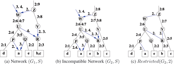
Figure 1.
In (a) & (b) G1 and G2 have segmentation S = {2, 3, 4}. (b) The two parents of node 'R' have labels {4, 2} and {3, 2}. Thus, the network restricted to segment label 2, shown in (c), has a closed path defined by the nodes labeled 'Z', 'W', 'U', 'R' and 'V'. Hence the network in (b) is not compatible.
For a segment s ∈ S, Restricted(G, s) is the network obtained by doing the following two operations:(1) Removing all recombination edges in G that do not have the element s in the true edge label lbl'. (2) From each mutation edge label in G, removing the elements of the form s: f, for any f, from the edge label. For a concrete example see Figures 1(b) and 1(c). This definition is easily extended to multiple segments as Restricted(G, S'), where S' ⊆ S.
G is always associated with a segmentation S of the F features, hence written as (G, S). Note that G cannot be any arbitrary network. It must satisfy the following: for each s ∈ S, Restricted(G, s) is devoid of recombinations. Such a network is termed compatible. The Consensus Compatible Network Problem is defined as follows [5]: Given two compatible networks (G1, S1) and (G2, S2) with no common features (thus S1 ∩ S2 = ∅), the task is to compute a compatible network (G3, S1∪ S2) with the minimum number of additional recombination nodes such that (G1, S1) is isomorphic to Restricted(G3, S1) and (G2, S2) to Restricted(G3, S2).
In the remainder of the paper, we refer to (G, S) simply as G, and segmentation S will be clear from context.
The Dominant Subdominant Recombinant (DSR) framework
The DSR scheme to solve the problem and its proof of correctness was presented in [5]. The method is an iterative, bottom-up working at one level of G1 and G2 at a time. The level of a node is defined as the maximum distance to a leafnode.
The same level is also associated with any edge e incident on the node written as level(e, G). A leaf is at level 0. The method gets its name from the need to give one of three possible assignments, Dominant (D) or Subdominant (S) or Recombinant (R), to nodes at each iteration, which is central to this scheme.
Matrix Xl
Let G have t roots. For root vi introduce an incoming edge ei, 1 ≤ i ≤ t. Then the height of G is defined as (level(ei, G)). Let lmax (lmin) be the maximum (minimum) of the heights of G1 and G2. For a fixed level l, let (i = 1, 2), = {e is an edge in Gi | level(e, Gi) = l}. Then intersection nl × ml matrix Xl is defined as and an example is shown in Fig 2. In the algorithm the intersection matrix, Xl had dimensions (nl + 1) × (ml + 1) as this extra last row (column) with header '-ϕ-' is required to take care of elements that are not covered by the rest of the columns (or rows). An empty entry is shown as '∅'. In X1 the exact entries can be computed and for Xl, l > 1 and the non-empty entries are identified by '{·}'. Further, let xl be the number of non-empty entries in Xl. See Figure 2 for an example.
Figure 2.
Given trees T1 in (a) and T2 in (b), each of height 3. (c) These two trees define Xl, 1 ≤ l ≤ 3, for each level l. Note that the entries in Xl, l > 1 differ in details depending on the choices the DSR algorithm makes. While '∅' denotes an empty set, '?' (including '{·}') could be either empty or non-empty, again depending on the choices the DSR Scheme makes.
DSR assignment rules
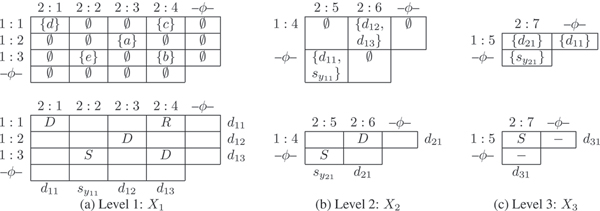
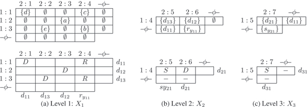
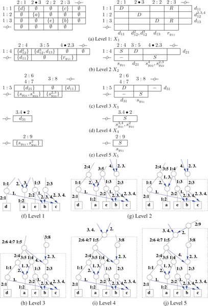
The non-empty entries of Xl are given a DSR assignment. Note that at least two conditions are required for a viable compatible network G3. (Rule 1): Each row (column) in matrix Xl has at most one dominant. If the row (column) has no dominant, then it has at most one subdominant. (Rule 2): A non-recombinant element can have another non-recombinant in its row or its column but not both. As a result of the DSR assignments to the entries on Xl, the rows and columns also get implicitly assigned as follows. A row (column) that has a dominant entry is assigned dominant. A row (column) that is not assigned dominant but has a subdominant in the row (column) gets assigned subdominant. A row (column) that has only recombinants in the row (column) is assigned recombinant. Note that only dominant rows (columns) contribute to entries in Xl', l' > l. Figures 4 and 5 give two different assignments giving the two different networks in Figure 3 (a) and (b) respectively. Using a simple greedy optimization approach, we include a third rule. (Rule 3): Minimize the number of recombinants in Xl. Complete examples are worked out in Figures 4, 5, 6 and 7 for the interested reader.
Figure 4.
X-matrices of Network G1 of Figure 3(a). The Xl matrix is shown on the top and the DSR assignment shown in the bottom row for each l, 1 ≤ l ≤ 3.
Figure 5.
X-matrices of Network G2 of Figure 3(b). Also see Figure 4 for a description of the matrices.
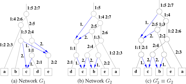
Figure 3.
(a) & (b) Two possible consensus networks G1 and G2 for two input trees T1 and T2 of Figure 2. (c) The edge labels of G2 have been locally shuffled keeping the exact same topology.
Figure 6.
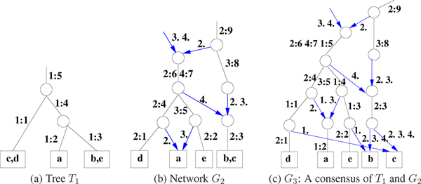
Consensus of a tree and a network.
Figure 7.
Stepwise construction of G3 of Figure 6(c) as consensus of T1 and G2: (a)–(e) The X matrices and the DSR assignments. (f)–(j) The construction of G3 using the DSR assignments of (a)–(e).
Approximation factor of the greedy DSR scheme
In this section, we compute the approximation factor [8,9] of the greedy version of the DSR Scheme. Let the number of new recombination events produced by the DSR algorithm in G3 be NDSR. Let the optimal number of new recombinations be Nopt. We use the following definition of the true approximation factor:
| (1) |
For given graphs G1 and G2 let zl = max(nl, ml) where nl > 0 and ml > 0 are the number of nodes at level l in G1 and G2 respectively. Further, let Z be the sum of all zl over all the levels (excluding the leaf level). Let Lv(G) be all the leafnodes (extant units) reachable from node v in G. For each level, l > 0, i.e. excluding the leafnodes, consider (G1), 1 ≤ i ≤ nl, where each vi is at level l in G1. Similarly consider (G2), 1 ≤ i ≤ ml, where each ui is at level l in G2. Let xl be the number of non-empty intersections between the two collection of sets and let Y be the sum of xl over all the levels (excluding leaf level). Note that if G1 and G2 are the same (isomorphic) graphs then Y = Z and Nopt = 0.
Theorem 1
| (2) |
Proof: Let Nmax (Nmin) be the maximum (minimum) number of new recombinations produced by the DSR scheme over all possible DSR assignments. Then we first show the following:
| Nmin≤ Nopt≤ NDSR≤ Nmax. | (3) |
Clearly Nopt≤ Nmax holds (else it contradicts the optimality of Nopt). Next we have to show that Nmin ≤ Nopt holds as well. For this we need a few more characterizations of the network.
Recombination node descriptor F1|F2
Let Y be the set all given haplotypes (or taxa). A split or bipartition is written as Z1|Z2 where Z1 and Z2 are nonoverlapping subsets of Y with Y = Z1∪ Z2. A tripartition Z1|Z2|Z3 is defined similarly. In earlier works (see [7,2] and citations therein) a mutation event has been associated with a bipartition of Y and a recombination event with a tripartition. However, the latter requires certain restrictions in the form of network G, i.e., a recombination node cannot be a direct descendent of another recombination node. Here we define recombination nodes as a bipartition of an appropriate subset of features.
For a fixed segment s, let s-path be a path in the graph with mutation edge(s) and recombinant edge(s) with s in its label. For any v, note that there is a unique s-path from a root to v. Further, let v be a recombination node and lbl1 and lbl2 be the labels of the two incoming (recombination) edges u1v and u2v respectively. For s1 ∈ lbl1 but s1 ∉ lbl2, let feature f1 be such that s1 : f1 is in the label of the closest mutation edge on the s1-path from v. Then F1 is the set of all such features. F2 is defined similarly. For example in G1 of Figure 1(a), consider the recombination leafnode labeled with haplotype a. Here lbl1 = {2}, lbl2 = {3} and the descriptor for this node is F1|F2 = {2:4}|{3:5}. For the recombination node labeled 'R', lbl1 = {4}, lbl2 = {2, 3} and the descriptor is F1|F2 = {4:7} | {2:9, 3:8}.
Isomorphism (G1 ≡ G2))
Let Lv(G) be all the leafnodes (extant units) reachable from node v. Let s: f be in the label of the unique incoming edge on mutation node v and then let Ls: f (G) be the same as Lv. Two compatible networks G1 and G2 on the same segmentation S are isomorphic (or identical), written as G1 ≡ G2, if the following two conditions hold: (1) For each element s: f in G1, Ls: f (G1) = Ls: f (G2) and viceversa, and, (2) For each recombination node v in G1 with descriptor F1|F2, there exists a recombination node in G2 with the same descriptor and viceversa.
Canonical form
It is possible to bubble up or down an element in the mutation edge label to obtain G' such that G' ≡ G. Our convention will be to bubble down the element of the mutation edge label, towards a leafnode. A network G is in the canonical form (1) if no node has only one outgoing edge and (2) if no element of any mutation edge label can be bubbled down to obtain G' with G' ≡ G. For example see Figure 3. Since the levels of nodes in a canonical network are unique, the following can be readily verified (see also concrete examples in Figures 2 and 6).
Lemma 1 Let G3 be the consensus of G1 and G2 which are in canonical forms, with lmax (lmin) as the maximum (minimum) of the heights of G1 and G2. Then there exist some X-matrices, X1, X2,..., whose DSR assignments produce G3. This is written as G3 ≅ X1, X2, ...,.
Back to the proof: We have to show that Nmin ≤ Nopt holds. Assume the contrary, i.e., Nopt <Nmin. In other words, the optimal number of new recombinations is even lower than the minimum produced by the algorithm over all possible choices. Then consider this network with Nopt new recombinations. Then by Lemma 1, there exist a sequence of X-matrices ≅ X1, X2, ..., with some DSR assignments for each Xl. Thus by these choices of the algorithm Nmin ≤ Nopt must hold, again leading to a contradiction.
Hence Nopt ≮ Nmin. Here ends the proof of correctness of Eqn 3. Next, we give a few characterizations of
the DSR assignment to facilitate the counting of the new recombinations.
Type I & II (new) recombination events
Let v be a recombination node in G3 with labels lbl1 and lbl2 on the two incoming edges and descriptor F1|F2. The recombination event is new if, without loss of generality, lbl1⊆ S1 and lbl2⊆ S2. In other words, this recombination node is a result of the consensus of G1 and G2 (and not a recombination that existed in G1 or G2). A new recombination node v is of two types: Let e1 (e2) be a mutation edge in G1 (G2) with a label in F1 (F2). Without loss of generality, let level(e1, G1) = l. Then the recombination is of Type I at level l if level(e2, G2) = l and is of Type II at level l if level(e2, G2) > l. Further, let the number of (non-empty) entries assigned dominant be , subdominant be and recombinant be in an X-matrix Xl. Then the following can be verified.
Lemma 2 The number of Type I recombination events at level l in G3 is . The number of Type II recombination events at level l in G3 is ≤ . Also, the number of recombination events in a network is bounded below (Nmin) by the number of Type I recombination events and above (Nmax) by the sum of the number of Type I and Type II recombination events.
Islands in X
We now give tighter bounds on , and for our analysis. Consider a bipartite graph B(V, E) with V partitioned into (1) nl nodes, corresponding to the rows and (2) ml nodes corresponding to the columns of Xl. The adjacency matrix is obtained from Xl where an empty set entry is replaced with 0 and a non-empty set entry with 1. Let the number of connected components [10] of graph B(V, E) be Cl. Each connected component corresponds to an island in Xl which is a collection of rows and columns of Xl. Thus Xl is fragmented into Cl islands, Xl,i, written as: Xl = Xl,1 + Xl,2 + ... + . See Figure 8 for an example. Note that this fragmentation is for analysis purposes only. Further, , for any yl,i, will be written simply as . Let island Xl,i have xl,i non-empty entries and let the number of entries assigned Y (D or S or R) in Xl,i be . Within an island the number of non-recombinants cannot exceed max(nl,i, ml,i) by Rules 1 and 2.
Figure 8.
(a) Xl has five rows and six columns. (b) The rows and columns have been permuted (shuffled) to reveal the three islands (or three connected components in the associated bipartite graph).
Lemma 3 For each island Xl,i:
| (4) |
| (5) |
Eqn 4 follows from using Rule 3 in island Xl,i and Eqn 5 from .
Back to the proof: Next, let Nc max(≥ Nmax) and Nc min(≤ Nmin) be some computable functions of the input (see Figure 9). Using Lemmas 2 and 3, we define appropriate (computable) Nc maxand Nc minas follows:
Figure 9.
The relative positions of the different counts on the real line. See text for details.
| (6) |
| (7) |
Note that the greedy Rule 3 encourages fragmentation of Xl, l > 1, into islands and under the best case scenario we get , which is used in Eqn 7 above. Finally, using Eqn 1, we have
| (8) |
The correctness of Eqn 2 is established by setting and . Here ends the proof.
Experimental results and discussion
In the last section we gave a mathematical proof of the tightness of the number of recombinations estimated by the model to explain the data. Also, in our earlier work we had presented results on simulation data with a general analysis of false positive and false negative errors. In this section, we discuss results on a segment of Chromosome X data and the plausibility of the results is verified independently by using traditional manual analysis. Due to the manual component in the verification process, here we use only small data sets.
Chromosome X SNP data
We used a 100 Kb segment of high SNP density in the recombining part of the X chromosome, starting at genomic position 87,348,404 (Build 35). In Hapmap II [11], this segment contains 194 sites, of which only 175 are polymorphic in at least one population. Recombination rate is ≈ 0.7 cM/Mb, slightly below the ≈ 1 cM/Mb genomewide average. We chose this segment for two reasons. (1) It does not contain any genes. Thus variation in this region is less likely to have been shaped by natural selection and is more likely to reflect purely genomic processes. (2) The segment does not contain copy number variations or segmental duplications. These could induce genotyping errors possibly producing ectopic recombination events, which is not accounted for in the downstream analysis.
Further, we used only the haplotypes in the hemizygous males to avoid any phasing errors. These errors would manifest as phantom recombination events. The populations used were Yorubans from Nigeria (YRI; N = 30), Europeans (CEU, N = 30), and a pooled sample of Chinese and Japanese (ASN; N = 45).
Statistical analysis (using p-value estimations)
As a preprocessing step, exploiting the coherence seen in the data, each haplotype is recoded using blocks of g SNPs. Based on the combinatorial model, a network is constructed from the recoded representative haplotypes. Recall that first the haplotype is segmented to give simple structures and then these individual structures are merged with a small number of recombinations to give a unified topology. Here we discuss the choice of the value of g in our experiments. Let l be the number of distinct patterns of the g SNPs across the samples. Using this as a proxy for the extent of LD in this block, we estimate the p-value of the number l. Loosely speaking, when these g SNPs are in linkage equilibrium (or independent), l should be much larger than when they are in LD.
Let the number of samples be H and let the number of SNPs be F. Further, let V be a column vector of size H. Since the SNPs are assumed to be bi-allelic, V which represents the value of a SNP in the H samples is binary. We use two schemes, based on the mode of definition of the F vectors, to estimates the p-value. The range of values of l seen in our data is 2 ≤ l < 15 and we study the p-value estimates in this range using two schemes.
RandV
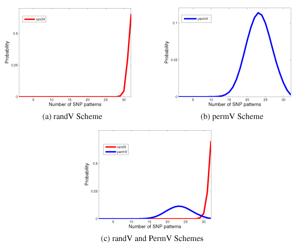
In this scheme, V1, V2, ..., VF are defined randomly. In other words, each entry of each V is picked independently and uniformly from a set of two alleles. We use 10000 replicates and the distribution of the number of g-sized patterns is shown in Fig 10. The p-values estimated based on this scheme is shown in the table below. The p-values are ≈ 0.0 for every value of l.
Figure 10.
Distribution of l for g = 5. Recall that the randV Scheme is independent of the region but the permV Scheme uses the population distribution of the region for a more realistic estimation.
PermV
While the RandV scheme is not incorrect, we make some domain-dependent modifications to design another scheme. In the PermV scheme we (i) mimic the allele frequencies seen in the input data and (ii) use the population distribution, by ethnicity, of the screened samples in the chromosomal region. The individual V vectors are plucked from the X-Chromosome of the database (but the SNPs span the entire chromosome) and any untyped SNP (i.e., N in the database) in the vector is given a value in agreement with the allele frequency of that column. Further, we use only those V 's that have MAF ≥ 0.1. We again use 10000 replicates and for each replicate, we randomly permute the F vectors. The distribution of the number of g-sized patterns is shown in Fig 10(b).
If for a block, l has an insignificant p-value, then the subsequent analysis risks becoming unreliable. We then reduce the grain size. An alternative is to discard the offending SNPs of the block, thus fragmenting the region. In our experiments we used a grain size g = 5 and the p-values obtained for this on all the regions were acceptable. The haplotypes are re-coded as sequence of these SNP patterns for the combinatorial analysis discussed in the Methods section.
Result analysis
We show a sample network of a short segment of the chosen region in Figure 11. Here we summarize our observations from a phylogeographic viewpoint and answer only questions raised traditionally in this area. Table 1 shows the number of detected recombination events and how they are shared across populations. The observations (over the entire 100 Kb segment) are as follows: We discovered a total of 31 recombinations in the data. Seventeen recombinations are population-specific, and can be used to infer the recombinational diversity within a population. Assuming recombination rate is constant across populations, this is a function of the effective population size of each population. Four recombinations are shared among pairs of populations, and can be used as indicators of shared population ancestry. In this particular case, both Europeans and Asians share events with the African population, which is more recombinationally diverse. Ten recombinations are shared among all three populations, and they are presumably ancient events that occurred before the split of the three populations.
Figure 11.
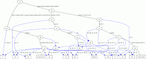
The network on segment Chr X: 87390235–87412114 of the three populations. The leafnodes are labeled with (a set of) clusters of the input haplotypes. A label on an internal node is for reference purposes only. An element of the edge label is to be interpreted as segment-id:position-id:pattern-id.
Table 1.
| CEU | ASN | YRI | |
| CEU | 2 | 0 | 1 |
| ASN | 4 | 3 | |
| YRI | 11 |
CEU & ASN & YRI: 10
Mutation-based studies of genetic diversity have shown exactly the same pattern: a larger diversity in Africans, and variation outside of Africa that is partially a subset of that in Africa. Our recombination-based results follow the same pattern, and, as the mutation data, fit the the "Out of Africa" model [12] for the origin of anatomically modern humans. Consistency with mutation data can be taken as an indirect validation of our analysis and the methodology. In our future work, we plan to investigate (raise as well as answer) more non-traditional questions.
Conclusion
We have addressed the problem of studying recombinational variations in human populations. One of the contributions of this work is a guaranteed upper bound on the approximation factor (ratio of discovered new recombination events to the true optimal) in a greedy polynomial time algorithm to construct a consensus network. Such an assurance is of significance when dealing with data where there are no other reasonable means of cross-checking results. To date, this bound is the best known result for this problem. We use this scheme to study recombinational imprints in an appropriate segment of X chromosome from three populations. While the upper bound on the approximation is our theoretical contribution, our second contribution is the results on this data: With our preliminary analysis, we are able to infer ancient recombinations, population-specific recombinations and more, which also support the widely accepted 'Out of Africa' model. The agreement with mutation-based analysis can be viewed as an indirect validation of our results and the methodology. In our future work, we plan to investigate more non-traditional questions via the networks computed by our methodology.
Competing interests
The authors declare that they have no competing interests.
Authors' contributions
The work is a result of the synergistic efforts of all the authors. However, the brunt of each author's involvement is as follows. Design and analysis of the mathematical models: LP. Design and implementation of the algorithms: AJ. Design and implementation of the experiments: MM, FC and JB. Further, LP and JB were involved in conceiving and planning the recombinations project.
Acknowledgments
Acknowledgements
We are thankful to Ajay Royyuru for his insightful comments on the work. We would also like to thank the anonymous referees for their helpful reviews.
This article has been published as part of BMC Bioinformatics Volume 10 Supplement 1, 2009: Proceedings of The Seventh Asia Pacific Bioinformatics Conference (APBC) 2009. The full contents of the supplement are available online at http://www.biomedcentral.com/1471-2105/10?issue=S1
Contributor Information
Laxmi Parida, Email: parida@us.ibm.com.
Asif Javed, Email: javeda@cs.rpi.edu.
Marta Melé, Email: marta.mele@upf.edu.
Francesc Calafell, Email: francesc.calafell@upf.edu.
Jaume Bertranpetit, Email: jaume.bertranpetit@upf.edu.
References
- Wilson EO. A consistency test for phylogenies based on contemporaneous species. Systematic Zoology. 1965;14:214–220. doi: 10.2307/2411550. [DOI] [Google Scholar]
- Semple C, Steel M. Phylogenetics. Oxford University Press; 2003. [Google Scholar]
- Hein J, Schierup MH, Wiuf C. Gene Genealogies, Variation and Evolution: A Primer in Coalescent Theory. Oxford University Press; 2005. [Google Scholar]
- Gusfield D, Hickersona D, Eddhua S. An efficiently computed lower bound on the number of recombinations in phylogenetic networks: Theory and empirical study. Discrete Applied Mathematics. 2007;155:806–830. doi: 10.1016/j.dam.2005.05.044. [DOI] [Google Scholar]
- Parida L, Melé M, Calafell F, Bertranpetit J, Genographic Consortium Estimating the ancestral recombinations graph (ARG) as compatible networks of SNP patterns. Journal of Computational Biology. 2008;15:1133–1154. doi: 10.1089/cmb.2008.0065. [DOI] [PubMed] [Google Scholar]
- Huson DH, Dezulian T, Klopper T, Steel MA. Phylogenetic super-networks from partial trees. IEEE/ACM TCBB. 2004;1:151–158. doi: 10.1109/TCBB.2004.44. [DOI] [PubMed] [Google Scholar]
- Moret BME, Nakhleh L, Warnow T, Linder CR, Tholse A, Padolina A, Sun J, R T. Phylogenetic networks: modeling, reconstructibility, and accuracy. IEEE/ACM TCBB. 2004;1:13–23. doi: 10.1109/TCBB.2004.10. [DOI] [PubMed] [Google Scholar]
- Arora S, Lund C. Hardness of approximations. PWS Publishing Company; 1996. pp. 399–446. [Google Scholar]
- Vazirani V. Approximation Algorithms. Springer; 2003. [Google Scholar]
- Cormen TH, Leiserson CE, Rivest RL. Introduction to Algorithms. Cambridge, Massachusetts: The MIT Press; 1990. [Google Scholar]
- HapMap Phase 2 http://www.hapmap.org
- Jobling MA, Hurles M, Tyler-Smith C. Human Evolutionary Genetics: Origins, Peoples and Disease. Garland Publishing; 2004. [Google Scholar]


