Bias in 2-part mixed models for longitudinal semicontinuous data

Abstract

Semicontinuous data in the form of a mixture of zeros and continuously distributed positive values frequently arise in biomedical research. Two-part mixed models with correlated random effects are an attractive approach to characterize the complex structure of longitudinal semicontinuous data. In practice, however, an independence assumption about random effects in these models may often be made for convenience and computational feasibility. In this article, we show that bias can be induced for regression coefficients when random effects are truly correlated but misspecified as independent in a 2-part mixed model. Paralleling work on bias under nonignorable missingness within a shared parameter model, we derive and investigate the asymptotic bias in selected settings for misspecified 2-part mixed models. The performance of these models in practice is further evaluated using Monte Carlo simulations. Additionally, the potential bias is investigated when artificial zeros, due to left censoring from some detection or measuring limit, are incorporated. To illustrate, we fit different 2-part mixed models to the data from the University of Toronto Psoriatic Arthritis Clinic, the aim being to examine whether there are differential effects of disease activity and damage on physical functioning as measured by the health assessment questionnaire scores over the course of psoriatic arthritis. Some practical issues on variance component estimation revealed through this data analysis are considered.

1. INTRODUCTION

1.1. Motivating example

Psoriatic arthritis (PsA) is a chronic inflammatory arthritis associated with psoriasis. The University of Toronto Psoriatic Arthritis Clinic has developed a prospective longitudinal observational cohort of patients with PsA since 1978 Gladman and others (1987). In a recent study, the investigators were interested in examining whether there are differential effects of disease activity and damage on physical functioning as measured by the health assessment questionnaire (HAQ) over PsA duration Husted and others (2007).

The HAQ is a self-report functional status (disability) measure that has become the dominant instrument in many disease areas, including arthritis Bruce and Fries (2003). It produces a measure that can take the value zero with positive probability, while nonzero values vary continuously in the range 0 (no disability) to 3 (completely disabled). Since June 1993, the HAQ has been administered annually to patients in the PsA clinic and, as of March 2005, 440 patients had completed at least one HAQ, with 382 (87%) completing 2 HAQs Husted and others (2007) and comprising the study group. In addition, at clinic visits, scheduled at 6–12 month intervals, demographic and other clinical information was obtained. There were 2107 HAQ observations available for our analyses. As shown in Figure 1, a notable feature of these data is the observation cluster at zero (645/2107 = 30.6%). This presents a challenge in characterizing the relationship between the HAQ scores and the explanatory variables.

Fig. 1.

Bar plot for the HAQ data in Section 1.1.

1.2. Models for longitudinal semicontinuous data

When an outcome variable is a mixture of true zeros and continuously distributed positive values, the data generated are termed “semicontinuous” Olsen and Schafer (2001). Various methods have been proposed for analyzing cross-sectional and longitudinal semicontinuous data Olsen and Schafer (2001), Berk and Lachenbruch (2002), Tooze and others (2002), Moulton and others (2002), Hall and Zhang (2004). It is natural to view a semicontinuous variable as the result of 2 processes, one determining whether the outcome is zero and the other determining the actual value if it is nonzero; for convenience, we refer to the data arising from these 2 processes as the “binary part” and the “continuous part” of the data, respectively. Two-part models are therefore attractive. In a 2-part model, it is assumed that explanatory variables influence the outcome through their role in the different processes. For example, for the HAQ data, interest may be in characteristics that distinguish PsA patients who had no difficulty in physical functioning (HAQ score = 0) from those who had at least mild difficulty (HAQ score > 0), and what characteristics have impact on the actual level of difficulty represented by positive HAQ scores, given that the patients had at least mild difficulty (HAQ score  > 0). In other words, the targets of inference are the distribution of the binary HAQ indicators and the conditional distribution of the HAQ scores given they are positive. In econometrics, 2-part models have been well developed for cross-sectional semicontinuous data Duan and others (1983), Zhou and Tu (1999), Tu and Zhou (1999). For longitudinal semicontinuous data, 2 approaches have been proposed recently. One is based on 2-part mixed models with correlated random effects in both parts of the model Olsen and Schafer (2001), Berk and Lachenbruch (2002), Tooze and others (2002). The other is based on 2-part marginal models using generalized estimating equation methodology Moulton and others (2002), Hall and Zhang (2004). Here, we focus on the former approach.

It is natural to conjecture that the 2 processes that generate semicontinuous data may be related, especially if the outcome is observed at multiple time points. For example, since no disability and low level of disability can both be features of mild PsA, clinically we would expect a low level of disability (positive HAQ score) on one occasion to be positively associated with the probability of having no disability (zero HAQ score) on another occasion. The introduction of correlated random effects is a means to account for both the dependence between observations within subjects and the dependence between the 2 processes in semicontinuous data. However, it can also lead to severe computational problems. For example, with many unstandardized explanatory variables and a long sequence of unbalanced longitudinal data Husted and others (2007), it may not be possible to obtain a fit using the SAS NLMIXED procedure (SAS Institute, Cary, NC, Version 9.1) within a reasonable time frame, probably due to the complexity of the specified model. In the analysis reported in Husted and others (2007), 2 of us (Brian D. M. Tom and Vernon T. Farewell) uncritically conjectured further that an incorrect assumption of independent random effects would not prevent consistent estimation of regression coefficients. Here, we correct this assumption and examine the impact of this correlation on the estimation of 2-part mixed models. The correlation is important because parameters in the model for the binary part determine the cluster size (e.g. the number of observations with positive HAQ score within subjects) for the continuous part of the model. Therefore, we are faced with an “informative cluster size” problem. Thus, the assumption of independence between random effects may produce bias in the estimation of both regression coefficients and variance components in the continuous part of the model for semicontinuous data.

The remainder of this article is organized as follows. Section 2 briefly summarizes 2-part mixed models for longitudinal semicontinuous data, including an extension to accommodate artificial zeros due to left censoring, and derives the asymptotic bias of parameter estimators when random effects are incorrectly assumed independent and other variance component parameters are fixed. In Section 3, we investigate the factors that influence the asymptotic bias derived in Section 2. The performance of 2-part mixed models in practice is considered in Section 4 using Monte Carlo simulations. The HAQ data are analyzed in Section 5, and some practical issues regarding variance component estimation are addressed in Section 6. We conclude with a discussion in Section 7.

2. BIAS IN 2-PART MIXED MODELS FOR SEMICONTINUOUS DATA

In this section, we briefly describe 2-part mixed models for semicontinuous data and their extension to accommodate artificial zeros Olsen and Schafer (2001), Berk and Lachenbruch (2002), Tooze and others (2002). We also discuss the potential bias for parameters in the continuous part.

2.1. Model assumptions

Olsen and Schafer (2001) first extended the 2-part model to the longitudinal setting by introducing correlated random effects into both the binary and the continuous parts of the model. Tooze and others (2002) discussed a similar 2-part mixed model.

Let Y_ij be a semicontinuous variable for the ith (i = 1,…,N) subject at time t_ij (j = 1,…,n_i). This outcome variable can be represented by 2 variables, the occurrence variable

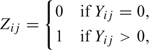and the intensity variable g(Y_ij) given that Y_ij > 0, where g(·) is a transformation that makes Y_ij∣Y_ij > 0 approximately normally distributed with a subject-time-specific mean.

Instead of focusing on the marginal distribution of Y_ij, in a 2-part mixed model we are interested in both the distribution for the occurrence variable Z_ij and the conditional distribution of the intensity variable g(Y_ij) given that Y_ij > 0. Specifically, it is assumed that Z_ij follows a random effects logistic regression model

(2.1)

where X_ij is a 1×q explanatory variable vector, θ is a q×1 regression coefficient vector, and U_i is the subject-level random intercept. The intensity variable g(Y_ij) given Y_ij > 0 follows a linear mixed model

(2.2)

where X_ij^* is a 1×p explanatory variable vector, β is a p×1 regression coefficient vector, and V_i is again a subject-level random intercept. The error term ∈_ij is assumed to be distributed as N(0,σ_e²). Note that this 2-part mixed model can be extended to include additional random effects. For simplicity, we restrict attention here to 2-part mixed models with random intercepts; extensions to models with random slopes will be discussed in Section 3.2.

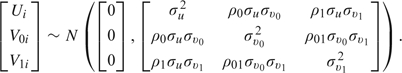
An important assumption is that the random intercepts, (U_i,V_i), are jointly normal and possibly correlated,

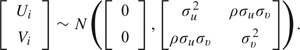(2.3)

In the context of the HAQ analysis introduced in Section 1.1, for example, the correlation aspect of this assumption can be interpreted as the presence or absence of disability at one occasion being related to the level of disability, if any, at that and other occasions.

In this model, the explanatory variable vectors X_ij, X_ij^* may coincide, but this is not required. The data can be unbalanced by design or due to ignorable missingness. The primary targets of inference are the regression coefficients θ and β, while variance components, including the correlation parameter ρ, are usually treated as nuisance parameters.

2.2. Model fitting

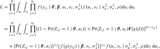
Generally, the estimation of θ, β, σ_u², σ_v², ρ, and σ_e² is based on maximization of the likelihood

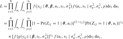(2.4)

which presents the same computational challenges as with generalized linear mixed models (GLMM) Stiratelli and others (1984), Breslow and Clayton (1993), Wolfinger and O'Connell (1993). Olsen and Schafer (2001) proposed an approximate Fisher scoring procedure based on high-order Laplace approximations for obtaining maximum likelihood estimates. Tooze and others (2002) used quasi-Newton optimization of the likelihood approximated by adaptive Gaussian quadrature and implemented it in the SAS PROC NLMIXED procedure. In the simulations and HAQ analysis in Sections 4 and 5, we use the same estimation procedure (SAS, 9.1) as in Tooze and others (2002).

2.3. Potential bias in 2-part mixed models

In practice, the multidimensional integration that is necessary to obtain the likelihood in (2.4) induces difficulties in fitting 2-part mixed models. In our HAQ analysis, we found that, even with properly standardized explanatory variables and the simplest model with 2 correlated random intercepts, it can take several hours to fit using the SAS NLMIXED procedure (1.5-GHz CPU, 1-Gb RAM, and SUN workstation). This is probably linked to the number of explanatory variables included in the model and the amount of data available for analysis. As a result, it may be impractical to conduct model assessment and selection procedures when a number of potentially important explanatory variables are available. However, if we assume independence between random effects, the likelihood components for the binary and continuous parts become separable Tooze and others (2002) and maximization of the likelihood is computationally much simpler and faster.

Nevertheless, as noted earlier, if the random effects are correlated, there is an informative cluster size aspect to the data structure since parameters in the binary part influence the number of observations in the continuous part of the model. Essentially, with a positive correlation, subjects with larger random effects V_i will have more observations contributing to estimation of the continuous part of the model; there will be an overrepresentation of larger values in this part of the data. Since we assume that E(V_i) = 0, an incorrect assumption of independence between random intercepts and the consequent analysis of the continuous part of the data separately from the binary part will produce positive bias in estimating the intercept term in β. The impact on estimation of other elements in β will depend on θ, σ_u², σ_v², ρ, σ_e², and the true value for β.

This scenario parallels the nonignorable missingness problem characterized in a class of “shared parameter models” Wu and Carroll (1988), Wu and Bailey (1989), Henderson and others (2000), Saha and Jones (2005). The model for the binary part in semicontinuous data corresponds to the logistic random effects model for missing indicators in shared parameter models, and the continuous part is similar to the partly unobserved outcome data modeled (typically) by linear mixed models. Underlying random effects in the shared parameter models link the models for missing indicators and outcomes, while in our case, the shared parameters are exactly those controlling correlated random intercepts (U_i,V_i) in (2.3). The only difference between these 2 scenarios is that in 2-part mixed models, both θ and β are primary targets of inference, whereas in shared parameter models only β in the outcome model is of interest.

For shared parameter models, Saha and Jones (2005) provided a useful procedure to quantify the asymptotic bias for estimating regression parameters in the outcome model when missingness is nonignorable and the missing data mechanism is not modeled jointly. Following Saha and Jones (2005), we can derive the asymptotic bias (as N goes to infinity) for estimating β in 2-part mixed models when the correlation ρ is nonzero but ignored (i.e. set to be zero) in estimation. We adopt the following notation:

• (A) n_i = J, the fixed number of observations within subjects;

• (B) X_ij = X_ij^* = (1,t_ij,G_i,G_it_ij) such that the explanatory variable vectors X_ij and X_ij^* both follow a group by time design and G_i∈(0,1) is a group membership indicator;

• (C) β^T = (β₀,β₁,β₂,β₃), true regression coefficients in the continuous part;

• (D) M_i, the pattern of occurrence variables (Z_i1,…,Z_iJ) that is observed for the ith subject;

• (E) Pr(M_i = m∣G_i = g), the probability that a subject in group g will have the mth occurrence indicator pattern;

• (F) X_m,g and Z_m,g, the fixed-effects design matrix and the random-intercepts design vector in the continuous part for the subjects in group g who have the mth occurrence indicator pattern;

• (G) Var{g(Y_ij)∣Y_ij > 0,M_i = m,G_i = g} = Ω_m,g = Z_m,gΛZ_m,g^T + σ_e²I, where Λ = σ_v²11^T, 1 is a vector of 1s, and I is the identity matrix;

• (H)β_m^T = (β_0m,β_1m,β_2m,β_3m), the regression coefficients for the continuous part given that the ith subject in group g has the mth occurrence indicator pattern, where β_0m = β₀ + E(V_i∣M_i = m,G_i = 0), β_1m = β₁, β_2m = β₂ + E(V_i∣M_i = m,G_i = 1) − E(V_i∣M_i = m,G_i = 0), β_3m = β₃, and V_i is the random intercept as in (2.3).

Further, for illustration, we assume that subjects have equal probability of being in the 2 groups, in other words, Pr(G_i = g) = 1/2 (g = 0,1), and that variance component parameters σ_u², σ_v², ρ, and σ_e² are known. It follows by equation (12) in Saha and Jones (2005) that the separate maximization of the likelihood for the continuous part (ρ = 0) will give estimates of β:

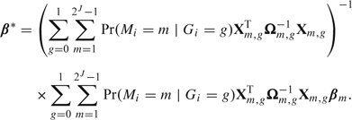(2.5)

Therefore, the absolute asymptotic bias of this estimation procedure is β^* − β, which is a function of θ and σ_u², σ_v², ρ, and σ_e². Because we assume that the continuous part of the model is specified by a linear mixed model and the variance components are known, the asymptotic bias derived here is independent of the true value of β. In practice, variance components also need to be estimated, and the asymptotic bias for estimating β in misspecified 2-part mixed models will depend on the true value of β. In that case, iterative methods are necessary to evaluate the asymptotic bias, as no analytical expression is available Saha and Jones (2005).

To compute (2.5), we need to evaluate Pr(M_i = m∣G_i = g) and E(V_i∣M_i = m,G_i = g). These can be shown to be

(2.6)

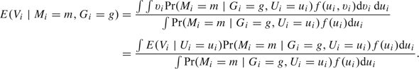(2.7)

The integrals in (2.6) and (2.7) are analytically intractable. In Section 3.1, we use a 30-point Gaussian quadrature Stroud and Secrest (1966) to evaluate them.

2.4. Artificial zeros

In practice, zero values from observed data can be a mixture of true zeros and artificial zeros due to left censoring. Berk and Lachenbruch (2002) discussed 2-part mixed models for dealing with this type of data. Specifically, following the notation in Section 2.1 and assuming that there is a detection limit d for the continuous part, the likelihood for the 2-part mixed model with additional artificial zeros is

(2.8)

where F is the cumulative distribution function for g(Y_ij)∣Y_ij > 0.

The same argument for potential bias as before can be applied to this 2-part mixed model with artificial zeros when the correlation between random intercepts is ignored. However, the derivation of asymptotic bias in Section 2.3 is no longer directly applicable. In Section 4, we will investigate bias using Monte Carlo simulations. It should be noted that there is minimal computational gain from assuming independence between random effects here as for the model with true zeros only because in this case the likelihood contributions for the binary and continuous parts cannot be disentangled and higher dimensional numerical integration is necessary for maximum likelihood estimation.

3. QUANTIFICATION OF ASYMPTOTIC BIAS

3.1. Two-part mixed model with random intercepts

In this section, we quantify the asymptotic bias in the estimation of β in the misspecified 2-part mixed models with random intercepts only assuming that all variance component parameters are known. Let t_ij = 0,1 denote the 2 measurement times for each subject and G_i = 0,1 denote a treatment indicator. We assume that subjects are equally likely to be assigned to the 2 groups and that

• (A) logit{Pr(Z_ij = 1)} = θ₀ + θ₁t_ij + θ₂G_i + U_i,

• (B) conditional on Y_ij > 0, [log(Y_ij)∣Y_ij > 0]∼N(β₀ + β₁t_ij + β₂G_i + V_i,σ_e²), and

• (C) (U_i,V_i) follow the bivariate normal distribution (2.3).

Recall that in (2.5), the asymptotic bias for estimating β depends on θ (or equivalently, the proportion of nonzero values for a typical subject in the subject groups), the correlation parameter ρ, the between-subject variability of occurrence variables σ_u², the between-subject variability of nonzero values σ_v², and the error variance of nonzero values σ_e². Given that the variance components are fixed in this specific scenario, the bias for β is independent of the true value of β.

For simplicity, we fix θ₁ = − 1 and θ₂ = log(2). Also, we fix σ_e² = 0.08 based on the HAQ analysis reported in Section 5. We then investigate how the asymptotic bias varies as a function of θ₀, σ_u², σ_v², and the correlation parameter ρ.

Figure 2 presents the contour plots of absolute asymptotic bias in estimation of the intercept term β₀ by σ_u² and the intraclass correlation ψ = σ_v²/(σ_v² + σ_e²) at different combinations of (θ₀,ρ). The axes for σ_u² and ψ are centered at 4 and 0.4, respectively, based on the HAQ analysis reported in Section 5. It is apparent from Figure 2 that β₀ is overestimated and the magnitude of the bias is positively related to ρ, σ_u², and σ_v² (or equivalently ψ). On the other hand, as θ₀ (the proportion of nonzero values in a control subject) increases, the bias in the estimation of β₀ decreases.

Fig. 2.

Contour plots of asymptotic bias for the intercept term β₀ in misspecified 2-part mixed model in Section 3.1 by occurrence random-intercept variance σ_u² and intraclass correlation ψ = σ_v²/(σ_v² + σ_e²), stratified by correlation between random effects (ρ = (0.2,0.5,0.8)) and overall proportion of zeros (i.e. intercept term in the binary part θ₀ = ( − 0.5,0.5,1.5); (θ₁,θ₂) = ( − 1,log(2)) are fixed). The error variance is fixed at σ_e² = 0.08

We also investigated absolute asymptotic bias in estimating the time effect β₁ and treatment effect β₂. A positive bias for β₁ and a negative bias for β₂ are observed, but the magnitudes of both biases are much smaller than for β₀. Details are given in Section 1.1 of the supplementary material available at Biostatistics online (http://www.biostatistics.oxfordjournals.org).

3.2. Two-part mixed model with random intercept and slope

As pointed out by a referee, it may be of interest to go beyond the simple 2-part model with random intercepts only and investigate the extended model where a random slope for time is included in the continuous part. Following the notation in Section 2.3, we now assume that

where X_ij^* = (1,t_ij,G_i,G_it_ij), V_0i, and V_1i are random intercept and random time slope, respectively. Similarly to (2.3), we assume that the random intercepts and additional random slope follow

(3.1)

In our HAQ example, the correlation ρ₁ under this assumption can be interpreted as the presence or absence of disability at one occasion being related to the rate of change in the disability level over time. For example, we would expect that patients who usually report no disability are unlikely to have large changes in the disability level when any disability is actually reported.

To derive the asymptotic bias for β, we follow the development in Section 2.3. The regression coefficients for the continuous part, given that the ith subject in group g has the mth occurrence indicator pattern, β_m, now changes to β_0m = β₀ + E(V_0i∣M_i = m,G_i = 0), β_1m = β₁ + E(V_1i∣M_i = m,G_i = 0), β_2m = β₂ + E(V_0i∣M_i = m,G_i = 1) − E(V_0i∣M_i = m,G_i = 0), and β_3m = β₃ + E(V_1i∣M_i = m,G_i = 1) − E(V_1i∣M_i = m,G_i = 0). To compute (2.5), we need to evaluate Pr(M_i = m∣G_i = g), E(V_0i∣M_i = m,G_i = g), and E(V_1i∣M_i = m,G_i = g). Since the model for the binary part does not change, Pr(M_i = m∣G_i = g) still follows (2.6). In addition, we can show that

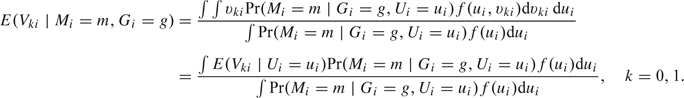(3.2)

We again use Gaussian quadrature to evaluate these integrals.

We use the same data structure as in Section 3.1 except that [log(Y_ij)∣Y_ij > 0]∼N(β₀ + β₁t_ij + β₂G_i + V_0i + V_1it_ij,σ_e²), and the random intercepts and slope (U_i,V_0i,V_1i) follow a trivariate normal distribution as in (3.9). We draw similar contour plots as in Section 3.1 to examine the asymptotic bias for the intercept term β₀, the time effect β₁, and the treatment effect β₂. We find that there are large positive biases for β₀ and β₁ and smaller negative bias for β₂ when the positive correlations increase and θ₀ decreases. Details are given in Section 1.2 of the supplementary material available at Biostatistics online.

4. MONTE CARLO SIMULATION

Simulation studies were done to investigate the performance of different 2-part mixed models in practice. For semicontinuous data with true zeros only, biases of different magnitude are observed for the regression coefficients in the continuous part of the model when the positive correlation of the random effects is ignored. In addition, the variance component in the continuous part is underestimated. For the data with additional artificial zeros, we observe biases for regression coefficients and variance components in both the binary and the continuous parts when the correlation is set to zero. Details are given in Section 2 of the supplementary material available at Biostatistics online.

5. ANALYSIS OF THE HAQ DATA

The HAQ data described in Section 1.1 can be modeled using a 2-part mixed model. The random-intercept logistic model (2.1) is used to model a binary indicator of a nonzero HAQ score, and the random-intercept linear mixed model (2.2) is used for nonzero HAQ scores. For the linear mixed model, residual plots suggest a symmetric error distribution. Thus, no transformation is applied to the nonzero HAQ scores and the results are therefore comparable to those in Husted and others (2007), where these data were modeled with an assumption of independent random intercepts. We refit this simple model and term it the “misspecified model.”

The same set of explanatory variables is included in both model parts, but the coefficients are allowed to differ. These include age at onset of PsA (standardized), sex, PsA disease duration in years, total number of actively inflamed joints, total number of clinically damaged joints, psoriasis area and severity index (PASI) score (standardized), morning stiffness (coded as either present or absent), standardized erythrocyte sedimentation rate (ESR), and highest medication level ever used prior to a visit, grouped based on a medication pyramid Gladman and others (1995), Munro and others (1998). Since there is particular interest in differential effects of both the number of actively inflamed joints and the number of clinically deformed joints on physical functioning over PsA duration, interaction terms for PsA duration with both variables are included in the model.

Prior to formal model fitting, an empirical check casts doubt on the assumption of independent random effects. When the empirical Bayes estimates of the random intercepts in the binary part are introduced as an additional explanatory variable in the linear mixed model for the continuous part, the associated coefficient is significantly positive (p < 0.001). Thus, we also fit a 2-part mixed model with correlated random intercepts (referred to as the “full model”). For estimation, the SAS NLMIXED procedure was used with the maximum number of adaptive Gaussian quadrature points in the quasi-Newton algorithm held at 31. The results are given in Tables 1 and 2.

Table 1.

Parameter estimates in the binary part of the model for the HAQ data

Parameters	Misspecified model		Full model		Latent process model
	Estimate (SE)	p	Estimate (SE)	p	Estimate (SE)	p
Intercept	– 1.0199 (0.4079)	0.0129	– 1.0015(0.3746)	0.0078	– 0.9909(0.3556)	0.0056
Age at onset of PsA	0.6031 (0.1743)	0.0006	0.6266(0.1611)	0.0001	0.6392(0.1538)	< 0.0001
Sex
Male
Female	1.9944(0.3603)	< 0.0001	2.0080 (0.3276)	< 0.0001	2.0037(0.3149)	< 0.0001
PsA disease duration	– 0.0027 (0.0259)	0.9169	0.0156(0.0232)	0.5027	0.0166(0.0220)	0.4501
Actively inflamed joints	0.1758 (0.0513)	0.0007	0.1566(0.0495)	0.0017	0.1380(0.0465)	0.0032
Clinically deformed joints	– 0.0161 (0.0321)	0.6165	0.0120(0.0260)	0.6441	0.0179(0.0238)	0.4531
PASI score	0.1941 (0.1257)	0.1233	0.1754(0.1086)	0.1071	0.1543(0.1017)	0.1299
Morning stiffness
No
Yes	1.5953 (0.2319)	< 0.0001	1.5777(0.2112)	< 0.0001	1.5691(0.2018)	< 0.0001
ESR	0.3030 (0.1310)	0.0213	0.2988(0.1164)	0.0106	0.2971(0.1103)	0.0074
Medications
None
NSAIDs	0.2998 (0.2743)	0.2751	0.2955(0.2529)	0.2435	0.2960(0.2439)	0.2257
DMARDs	0.3074 (0.2508)	0.2211	0.3100(0.2295)	0.1776	0.3138(0.2197)	0.1541
Steroids	0.9945 (0.4698)	0.0350	0.9946(0.4458)	0.0263	0.9927(0.4355)	0.0232
Interaction of actively inflamed	0.0002 (0.0034)	0.9502	– 0.0003(0.0033)	0.9403	0.0003(0.0031)	0.9300
joints with arthritis duration
Interaction of clinical deformed	0.0032 (0.0016)	0.0442	0.0022(0.0013)	0.0844	0.0018(0.0011)	0.1102
joints with arthritis duration
σu2	4.2519 (0.8549)	< 0.0001	4.3930(0.8924)	< 0.0001	4.2641(0.9001)	< 0.0001
ρ	(ρ = 0)		0.9423(0.0373)	< 0.0001	(ρ = 1)

SE, standard error.

Table 2.

Parameter estimates in the continuous part of the model for the HAQ data

Parameters	Misspecified model		Full model		Latent process model
	Estimate (SE)	p	Estimate (SE)	p	Estimate (SE)	p
Intercept	0.3176(0.0567)	< 0.0001	0.2149(0.0556)	0.0001	0.1748(0.0555)	0.0018
Age at onset of PsA	0.1011(0.0242)	< 0.0001	0.1009(0.0245)	< 0.0001	0.0984(0.0250)	0.0001
Sex
Male
Female	0.1811(0.0505)	0.0004	0.2225(0.0512)	< 0.0001	0.2461(0.0523)	< 0.0001
PsA disease duration	0.0039(0.0033)	0.2272	0.0035(0.0032)	0.2726	0.0044(0.0032)	0.1719
Actively inflamed joints	0.0219(0.0028)	< 0.0001	0.0239(0.0027)	< 0.0001	0.0243(0.0027)	< 0.0001
Clinically deformed joints	0.0058(0.0031)	0.0627	0.0052(0.0031)	0.0957	0.0051(0.0031)	0.1034
PASI score	0.0128(0.0140)	0.3636	0.0247(0.0134)	0.0667	0.0257(0.0134)	0.0553
Morning stiffness
No
Yes	0.1502(0.0274)	< 0.0001	0.1573(0.0263)	< 0.0001	0.1620(0.0262)	< 0.0001
ESR	0.0395(0.0132)	0.0028	0.0388(0.0127)	0.0024	0.0374(0.0126)	0.0033
Medications
None
NSAIDs	– 0.0240 (0.0289)	0.4065	– 0.0177(0.0281)	0.5288	– 0.0181(0.0280)	0.5194
DMARDs	0.0224(0.0280)	0.4252	0.0235(0.0272)	0.3889	0.0226(0.0272)	0.4064
Steroids	0.0457(0.0453)	0.3135	0.0493(0.0441)	0.2641	0.0481(0.0441)	0.2761
Interaction of actively inflamed	– 0.0004(0.0002)	0.0290	– 0.0004(0.0002)	0.0072	– 0.0005(0.0002)	0.0042
joints with arthritis duration
Interaction of clinical deformed	0.0002(0.0001)	0.1122	0.0003(0.0001)	0.0330	0.0003(0.0001)	0.0351
joints with arthritis duration
σv2	0.1587(0.0154)	< 0.0001	0.1732(0.0166)	< 0.0001	—	—
σv/σu	—	—	—	—	0.2074 (0.0210)	< 0.0001
σe2	0.0785(0.0040)	< 0.0001	0.0774(0.0039)	< 0.0001	0.0779(0.0039)	< 0.0001
ρ	(ρ = 0)		0.9423(0.0373)	< 0.0001	(ρ = 1)
– 2 log- likelihood (both parts)		2116.0		2018.1		2022.2
AIC		2178.0		2082.1		2084.2

SE, standard error.

As shown in Table 1, the estimated coefficients in the binary part are approximately the same in both the full and the misspecified models and suggest the same explanatory variables of functional difficulty. There is no differential effect of actively inflamed joints on functioning difficulty over PsA duration, but some evidence that the effect of deformed joints increases with disease duration. The parameter estimates for the random-intercept distribution in the binary part are also similar.

The estimated correlation between random intercepts of the 2 parts of the full model is positive and close to one (). This large estimate suggests that there might be a single unmeasured latent process which influences the 2 processes of the mixed model, corresponding to perfectly correlated random intercepts. Therefore, we also fit a 2-part model such that the correlated random intercepts follow V_i = αU_i and σ_v² = α²σ_u² and refer to this model as the “latent process model.” A similar approach is implemented in the Mplus software Brown and others (2005), Muthén and Muthén (1998–2007). The estimates from the binary part of this model are listed in the last 2 columns of Table 1 and are similar to those from the other 2 models.

As expected, the misspecified model overestimates the intercept term and underestimates the time-invariant sex effect in the continuous part (Table 2). For other time-varying explanatory variables, the estimates are approximately the same except that the coefficients for PASI score and the interaction between clinically deformed joints and PsA duration are larger in the full model, with correspondingly smaller p-values. The random-intercept variance of the continuous part in the misspecified model is underestimated and error variance estimates are similar, consistent with our simulation results. Thus, the qualitative conclusions do not change across models. In particular, the positive effects of actively inflamed joints and clinically deformed joints differ over PsA duration: the effect of the former decreases while the effect of the latter increases over time.

The deviance and Akalike Information Criterion (AIC) values in Table 2 indicate that the full model and latent process model provide a better fit to the data. A likelihood ratio test of the hypothesis of zero correlation generates a p-value less than 0.001.

6. REMARKS ON VARIANCE COMPONENT ESTIMATION IN 2-PART MIXED MODELS

In preliminary analysis, we observed that, with some important explanatory variables omitted (e.g. age at onset of PsA, sex, and ESR) in the binary part of the model, estimation of the random-intercept variance σ_u² becomes unstable. For example, its point estimate can increase from 6.9 in a misspecified model (ρ = 0) to 10.8 in a full model with estimated correlation ρ close to one. As a result, estimates of subject-specific regression coefficients θ are inflated in the full model. However, the corresponding standard error estimate of σ_u² also increases and ratio-based statistics are approximately the same in both models. This behavior was not evident in our simulation results. We suspect that the reason for this instability is that the unaccounted variability represented by the variance component is large, and the likelihood surface is flat for the estimation procedure to locate the maximum. This can be investigated further through examination of the profile likelihood for σ_u² under scenarios where σ_u² is large.

We simulated data with N = 250 subjects, with n_i = 2, from the same logistic-lognormal mixture distribution as in (2.1) and (2.2) of the supplementary material available at Biostatistics online. The true values for the parameters were set to θ = (3,0,0,0) (or θ = (0,0,0,0)), β = (0.5,0,0,0), σ_u² = 4.5 (or σ_u² = 10.5), σ_v² = 0.2, σ_e² = 0.08, and ρ = 0.9. In obtaining the profile likelihood for σ_u² and ρ, we fixed σ_v² and σ_e² at their true values and let θ and β be estimated.

Figure 3 presents the contour plots of the profile likelihood (in terms of the deviance) for σ_u² and ρ from 4 simulated data sets. The top-left panel in Figure 3 displays flat profile likelihoods for σ_u² at different levels of ρ when the true between-subject heterogeneity is large (σ_u² = 10.5) and the proportion of zeros in the data is small (θ₀ = 3). The black dots, which are the corresponding restricted maximum likelihood estimates for σ_u², show an increasing trend as ρ increases. With σ_u² = 10.5 still, but the proportion of zeros now increased (θ₀ = 0), the profile likelihood surface shows slightly more curvature. The situation improves further when the true variance decreases to σ_u² = 4.5, but restricted maximum likelihood estimates for σ_u² when θ₀ = 3 still vary considerably. In contrast, with θ₀ = 0, the likelihood appears to be well behaved and estimates for σ_u² are relatively constant. Therefore, the sparseness of the occurrence indicator data also impacts on variance component estimation in the binary part of the mixed model.

Fig. 3.

Contour plots of profile likelihood (in terms of the deviance) occurrence random-intercept variance σ_u² and correlation ρ from 4 simulated data sets (N = 250) with different combinations of true values for σ_u² and θ₀; other variance components are fixed at their true values σ_v² = 0.20 and σ_e² = 0.08; the true value for β₀ is set as β₀ = 0.5; the black dots are maximum likelihood estimates of σ_u² at different values of ρ

These results help to explain the instability observed in our preliminary analyses. With important explanatory variables omitted in the binary part, the unexplained variability in the indicator of a positive HAQ score was unduly large, estimation of σ_u² was unstable, and point estimates and standard errors changed as the correlation ρ increased. Consequently, the estimates for subject-specific regression coefficients θ differed across the models. With a reasonable set of important explanatory variables in the final HAQ analysis, the estimates for both σ_u² and θ were stabler.

In summary, careful modeling of mean relationships is necessary to avoid unstable estimation of variance components and subject-specific regression coefficients when fitting 2-part mixed models. When the number of zeros in longitudinal semicontinuous data is small, caution is advised in fitting 2-part mixed models. Simpler alternatives, such as standard regression methods for the marginal distribution of outcomes, either truncated or bounded, should be considered.

7. DISCUSSION

For 2-part mixed modeling of longitudinal semicontinuous data, with true zeros only or with additional artificial zeros due to left censoring, an incorrect assumption of independence between random effects can induce bias in the estimation of regression coefficients and variance components in the continuous part of the model. This arises due to differential representation of nonzero values in the continuous part of the data. For illustration, we examined linear mixed models for the continuous part of the model, but the same issues apply to other GLMM. Model fitting with correlated random effects is computationally expensive, and the availability of more efficient software would therefore be welcome.

As pointed out by an associate editor, the extreme computing time experienced in the HAQ analysis might be alleviated by adopting a marginal approach for a 2-part model. As shown in Section 6, variance component estimation in the binary part can be unstable when the unexplained variability is large. Computing time can be considerable due to the difficulty of locating the maximum of a flat likelihood surface. In this case, we may choose marginal 2-part models such as in Moulton and others (2002) and Hall and Zhang (2004) rather than the mixed model approach. However, we emphasize that for marginal 2-part models of longitudinal or even cross-sectional semicontinuous data, bias can also be induced if important explanatory variables determining both the binary process and the process of nonzero values are excluded in the model for the continuous part. These important explanatory variables in marginal models are similar to the unmeasured explanatory variables represented by correlated random effects in mixed models. Therefore, the same problem of differential representation of nonzero values in the continuous part can arise even when these omitted explanatory variables are independent of other included explanatory variables in the continuous part. Thus, when building a model for mean structures in these marginal models, any important explanatory variables in the binary part should be included in the continuous part, at least initially, to reduce the possibility of bias.

The HAQ data analysis presented in this article is primarily illustrative. Alternative models might be preferred. The normality assumption of random intercepts was examined using empirical Bayes estimates. However, as with shared parameter models Tsonaka and others (2008), diagnostic checks based on empirical Bayes estimates are unreliable due to shrinkage (Verbeke and Molenberghs, 2001, Section 7.8). In practice, investigators might be only interested in the continuous part of the data and thus fit regression models ignoring the zeros. The bias illustrated in this article is then still present due to the differential representation of nonzero values across patients. The change of the primary inference target from (β,θ) to β does not solve the problem.

FUNDING

Funding to pay the Open Access publication charges for this article was provided by Medical Research Council (UK) (U.1052.00.009).

References

- Berk KN, Lachenbruch PA. Repeated measures with zeros. Statistical Methods in Medical Research. 2002;11:303–316. doi: 10.1191/0962280202sm293ra. [DOI] [PubMed] [Google Scholar]
- Breslow N, Clayton D. Approximate inference in generalized linear mixed models. Journal of the American Statistical Association. 1993;88:9–25. [Google Scholar]
- Brown E, Catalano C, Fleming C, Haggerty K, Abbot R. Adolescent substance use outcomes in the Raising Healthy Children Project: a two-part latent growth curve analysis. Journal of Consulting and Clinical Psychology. 2005;73:699–710. doi: 10.1037/0022-006X.73.4.699. [DOI] [PubMed] [Google Scholar]
- Bruce B, Fries JF. The Stanford health assessment questionnaire: dimensions and practical applications. Health and Quality of Life Outcomes. 2003;1:1–20. doi: 10.1186/1477-7525-1-20. [DOI] [PMC free article] [PubMed] [Google Scholar]
- Duan N, Manning WG, Morris CN, Newhouse JP. A comparison of alternative models for the demand for medical care. Journal of Business and Economic Statistics. 1983;1:115–126. [Google Scholar]
- Gladman D, Farewell VT, Nadeau C. Clinical indicators of progression in psoriatic arthritis: multivariate relative risk model. The Journal of Rheumatology. 1995;22:675–679. [PubMed] [Google Scholar]
- Gladman DD, Shuckett R, Russell ML, Thorne J, Schachter RK. Psoriatic arthritis (PsA)––an analysis of 220 patients. The Quarterly Journal of Medicine. 1987;62:127–141. [PubMed] [Google Scholar]
- Hall DB, Zhang Z. Marginal models for zero inflated clustered data. Statistical Modelling. 2004;4:161–180. [Google Scholar]
- Henderson R, Diggle P, Dobson A. Joint modelling of longitudinal measurements and event time data. Biostatistics. 2000;1:465–480. doi: 10.1093/biostatistics/1.4.465. [DOI] [PubMed] [Google Scholar]
- Husted JA, Tom BD, Farewell VT, Schentag CT, Gladman DD. A longitudinal study of the effect of disease activity and clinical damage on physical function over the course of psoriatic arthritis: does the effect change over time? Arthritis & Rheumatism. 2007;56:840–849. doi: 10.1002/art.22443. [DOI] [PubMed] [Google Scholar]
- Moulton LH, Curriero FC, Barroso PF. Mixture models for quantitative HIV RNA data. Statistical Methods in Medical Research. 2002;11:317–325. doi: 10.1191/0962280202sm292ra. [DOI] [PubMed] [Google Scholar]
- Munro R, Hampson R, McEntegart A, Thomson EA, Madhock R, Capell H. Improved functional outcome in patients with early rheumatoid arthritis treated with intramuscular gold: results of a five year prospective study. Annals of the Rheumatic Diseases. 1998;57:88–93. doi: 10.1136/ard.57.2.88. [DOI] [PMC free article] [PubMed] [Google Scholar]
- Muthén LK, Muthén BO. Mplus User's Guide. 5th edition. Los Angeles, CA: Muthén & Muthén; 1998–2007. [Google Scholar]
- Olsen MK, Schafer JL. A two-part random-effects model for semicontinuous longitudinal data. Journal of the American Statistical Association. 2001;96:730–745. [Google Scholar]
- Saha C, Jones MP. Asymptotic bias in the linear mixed effects model under non-ignorable missing data mechanisms. Journal of the Royal Statistical Society, Series B. 2005;67:167–182. [Google Scholar]
- Stiratelli R, Laird N, Ware JH. Random-effects models for serial observations with binary response. Biometrics. 1984;40:961–971. [PubMed] [Google Scholar]
- Stroud AH, Secrest D. Gaussian Quadrature Formulas. Englewood Cliffs, NJ: Prentice-Hall; 1966. [Google Scholar]
- Tooze JA, Grunwald GK, Jones RH. Analysis of repeated measures data with clumping at zero. Statistical Methods in Medical Research. 2002;11:341–355. doi: 10.1191/0962280202sm291ra. [DOI] [PubMed] [Google Scholar]
- Tsonaka R, Verbeke G, Lesaffre E. A semi-parametric shared parameter model to handle nonmonotone nonignorable missingness. Biometrics. 2008 doi: 10.1111/j.1541-0420.2008.01021.x. doi: 10.1111/j.1541–0420.2008.01021.x. [DOI] [PubMed] [Google Scholar]
- Tu W, Zhou XH. A Wald test comparing medical costs based on log-normal distributions with zero valued costs. Statistics in Medicine. 1999;18:2749–2761. doi: 10.1002/(sici)1097-0258(19991030)18:20<2749::aid-sim195>3.0.co;2-c. [DOI] [PubMed] [Google Scholar]
- Verbeke G, Molenberghs G. Linear Mixed Models for Longitudinal Data. New York: Springer; 2001. [Google Scholar]
- Wolfinger R, O'Connell M. Generalized linear models. Journal of Statistical Computer Simulation. 1993;48:233–243. [Google Scholar]
- Wu M, Bailey K. Estimation and comparison of changes in the presence of informative right censoring: conditional linear model (corr:v46 p889) Biometrics. 1989;45:939–955. [PubMed] [Google Scholar]
- Wu M, Carroll R. Estimation and comparison of changes in the presence of informative right censoring by modeling the censoring process. Biometrics. 1988;44:175–188. [Google Scholar]
- Zhou XH, Tu W. Comparison of several independent population means when their samples contain log-normal and possibly zero observations. Biometrics. 1999;55:645–651. doi: 10.1111/j.0006-341x.1999.00645.x. [DOI] [PubMed] [Google Scholar]
Associated Data
This section collects any data citations, data availability statements, or supplementary materials included in this article.