Evaluating Predictors of Geographic Area Population Size Cut-offs to Manage Re-identification Risk

Abstract

Objective

In public health and health services research, the inclusion of geographic information in data sets is critical. Because of concerns over the re-identification of patients, data from small geographic areas are either suppressed or the geographic areas are aggregated into larger ones. Our objective is to estimate the population size cut-off at which a geographic area is sufficiently large so that no data suppression or further aggregation is necessary.

Design

The 2001 Canadian census data were used to conduct a simulation to model the relationship between geographic area population size and uniqueness for some common demographic variables. Cut-offs were computed for geographic area population size, and prediction models were developed to estimate the appropriate cut-offs.

Measurements

Re-identification risk was measured using uniqueness. Geographic area population size cut-offs were estimated using the maximum number of possible values in the data set and a traditional entropy measure.

Results

The model that predicted population cut-offs using the maximum number of possible values in the data set had R² values around 0.9, and relative error of prediction less than 0.02 across all regions of Canada. The models were then applied to assess the appropriate geographic area size for the prescription records provided by retail and hospital pharmacies to commercial research and analysis firms.

Conclusions

To manage re-identification risk, the prediction models can be used by public health professionals, health researchers, and research ethics boards to decide when the geographic area population size is sufficiently large.

Introduction

Privacy legislation in Canada applies to identifiable information. This means that if health information is deemed sufficiently de-identified, then there is no legislative requirement to obtain consent from patients to collect it and use it. ¹ In addition, Research Ethics Boards (REBs) are more likely to waive the consent requirement if the information collected for research is deemed de-identified. ² The option to waive consent is important as there is evidence that currently used methods for obtaining opt-in consent can result in low recruitment and selection bias in health research. ^3–10 The ability to make precise claims about identifiability therefore is needed to inform this consent waiver decision.

It is obvious that variables such as name and address would have to be removed, or not collected to start off with, to de-identify a data set. However, beyond the elimination of such variables, the definition of identifiability is often vague and remains an active area of research. ¹¹

The inclusion of geographic information (geocoding) in health data sets is critical for public health investigations and health services research. ^12–17 However, the inclusion of geographic details in a data set also makes it much easier to re-identify patients. ^18,19 The more specific the geographic detail included, the easier it is to use the other variables/information in the data to uniquely identify an individual. In fact, recently the federal court accepted evidence that the inclusion of the “Province” field in Health Canada's adverse drug events database can potentially re-identify individuals. ²⁰ Therefore, the province where the adverse event occurred cannot be disclosed by Health Canada in response to an access to information request. It has also been shown that patient addresses can be re-identified from published maps. ^21–23 Consequently, there is a risk that geographic detail in health data sets makes Canadians identifiable.

To protect privacy one can mask geocodes, ^24,25 or control geographic area population size (GAPS) to minimize the risk of re-identification. Due to its relative simplicity, controlling GAPS has been adopted widely in practice. Controlling GAPS means either that data about individuals living in areas with small populations are suppressed, or that areas with small populations are aggregated into larger ones. Suppression results in the direct loss of data, and aggregation reduces the utility of a data set. ^26–28 This is justified because of the demonstrated empirical relationship between GAPS and re-identification risk ^29–31 : re-identification risk tends to be higher in areas with smaller populations.

Examples of GAPS cut-off use include the United States Health Insurance Portability and Accountability Act (HIPAA) Privacy Rule. The HIPAA Privacy Rule defines 18 variables in the Safe Harbor List that need to be removed or generalized to ensure that a data set is de-identified. One of these 18 items stipulates that the first three numbers of the ZIP code can be collected/disclosed if the population living within that geographic area is greater than 20,000 people. The US Bureau of the Census has a 100,000 GAPS cut-off for releasing public use microdata files. ^32–34 That same cut-off is used for making disclosure control decisions with public health data sets. ^35,36 Only data from areas with a population of 120,000 or more are released as microdata from the British census. ³⁷ Similarly, Statistics Canada uses a 70,000 population size cut-off for health regions to control the risk of disclosure when releasing data from the Canadian Community Health Survey (CCHS). ³⁸ It has been suggested that different GAPS cut-offs should be applied depending on the user, with a 25,000 cut-off for data disclosed to researchers, and a 100,000 cut-off for data disclosed to the public. ³⁹

The dearth of evidence supporting the specific cut-offs that are used in practice, and the “real research need to develop empirical evidence to justify recommendations regarding geographic specificity” ¹⁹ make the continued search for GAPS cut-offs important. Furthermore, existing GAPS cut-offs do not account for the fact that a cut-off is inherently dependent on the number and nature of the variables under consideration. ^31,40 For example, the cut-off to apply when one has two variables will be smaller than a cut-off to apply when there are 15 variables. When the variables have few response categories, the cut-off will be smaller than when they have many response categories. Therefore, many GAPS cut-offs in current use (summarized above), may be overprotecting data sets or not protecting them enough depending on the specific variables in question.

The purpose of our study is to provide an empirically grounded basis for using GAPS cut-offs. The primary contributions of this work are to (a) provide models for predicting the GAPS cut-offs that explicitly account for re-identification risk and the variable characteristics based on two simple metrics: the number of possible combinations of data fields and entropy, (b) validating these models using Canadian census data, and (c) demonstrating their applicability with two examples of pharmacy prescription data.

Methods

Definitions and Preliminaries

Quasi-identifiers

When considering re-identification risk, we are only interested in a subset of variables in a data set. ⁴¹ These are called the quasi-identifiers. ⁴² They are variables that make individuals unique in the population and are possibly publicly known. Therefore, they do not directly identify an individual, but can be used for indirect re-identification. While there is no universal definition of what constitutes a quasi-identifier, there are some quasi-identifiers that have been studied more extensively than others such as gender, date of birth, ethnicity, income, years of education, and geocodes. In addition, quasi-identifiers may differ across data sets. For example, gender will not be a meaningful quasi-identifier if all of the individuals in a data set are female. Lastly, in this study, the quasi-identifiers that are assessed have a finite set of possible discrete values.

Uniqueness as a Measure of Re-identification Risk

We define a unique individual as the one individual with specific values on the quasi-identifiers in a particular geographic area. For example, if there is only one 95-year-old male in a postal code, then that individual is unique within that postal code. The uniqueness of individuals is often used as a surrogate measure for re-identification risk: unique records in a data set are more likely to be re-identified by an intruder than non-unique records. ⁴³ We therefore use uniqueness as our measure of re-identification risk.

Nested Geographic Areas

Geographic area aggregation implies a nesting relationship among those areas. For example, if we decide that re-identification risk is too high when we geocode using full postal codes, then we can aggregate the geographic area to Forward Sortation Areas (FSA), which are the first three characters of the postal code. Postal codes are nested within FSAs.

Determining the GAPS Cut-offs

Geographic areas can be measured in terms of the physical area or population size. In this paper we refer only to the population size of the geographic area.

Previous research has identified two characteristics of the relationship between uniqueness and GAPS: ^29–31

• • Uniqueness in a data set is inversely proportional to the population size of the geographic area. This means that the proportion of unique individuals in a large area will be smaller than in a nested smaller area. As smaller areas are aggregated into larger areas, the proportion of uniques goes down (see ▶).

• • Once GAPS reaches a certain point, uniqueness tends to plateau. This trend applies irrespective of the quasi-identifiers in question.

Figure 1.

Illustration of how the GAPS cutoff is calculated. Uniqueness is computed as the proportion of individuals who are unique on the values of the quasi-identifiers. For example, a uniqueness of 0.02 for a geographic area of 10,000 individuals on age, ethnicity, and gender means that 200 individuals have unique values on the combination of these three variables. At the limit, with an infinitely sized area, the uniqueness approaches zero. The delta value is the uniqueness at the GAPS cutoff value.

A case has been made that the 100,000 GAPS cut-off used by the Census Bureau is justified by computing the uniqueness plateau noted above (i.e., the point at which uniqueness no longer changes). ²⁹ The rationale is that increasing the size of the geographic area any further has little impact on uniqueness, and hence little impact on re-identification risk. ^29–31 For example, if the uniqueness plateau is reached at 100,000 then this means the re-identification risk changes insignificantly between 100,000 and 110,000. Therefore, there is no disclosure control benefit in increasing the size of the geographic region or of aggregation beyond 100,000, and a reasonable cut-off would be 100,000.

In our analysis we build on a methodology used in a previous study at the Census Bureau ^29,31 and proceed as follows:

• • Define a quasi-identifier model as a specific quasi-identifier or combination of quasi-identifiers and evaluate its uniqueness.

• • Plot uniqueness against GAPS and compute the cut-off point as the point where the derivative approaches zero (illustrated in ▶).

Let the geographic areas under consideration be indexed by 1..K, and their population size denoted by S_i where i:1..K. The area indexed by i is nested within the area indexed by i+1. Consequently, we also have S_i < S _i+1 for all i. We denote the percentage of individuals on a particular quasi-identifier model that are unique in an area i by U(S _i). Because of the monotonically decreasing relationship between GAPS and uniqueness, we expect the following relationship to hold: U(S _i) > U(S _i+1). The GAPS cut-off was then defined as the value of S_i where the approximate derivative, the change in the percentage of uniques, is close to zero ³¹ :

(1)

This approach, however, may identify local plateaus where the uniqueness remains temporarily steady, followed by a more substantial decrease to reach the asymptotic value. To address this we adopted a model building approach where the uniqueness function is defined as U(S_i) = β₀ × S _i ^β₁, where the β₀ and β₁ are estimated using ordinary least squares regression. We then take the derivative of this function and compute the cut-off as the size value where the derivative approaches zero:

(2)

The cut-off values were computed separately for central Canada (which includes Ontario and Quebec), western Canada (which includes all territories and provinces west of Ontario), and eastern Canada (which includes all provinces east of Quebec).

Data Source

The data set used for our study is the 2001 Canadian census Public Use Microdata File (PUMF) made available by Statistics Canada. ⁴⁴ The PUMF represents approximately 2.7% of the Canadian population. The variable subset that is analyzed is shown in ▶. These are common demographics that are often available in health data sets. There are 10 quasi-identifiers. These variables were selected because they can be used to link with other databases, because they describe attributes which are visible on individuals, or because they describe attributes which would make individuals easily identifiable. ⁴¹

Table 1.

Table 1 Quasi-identifiers to be Included in the Models for the Three Regions of Canada

		Number Response Categories ∗
Variable Name in the Census File	Definition	Western and Central Canada	Eastern Canada
SEXP	sex	2	2
AGEP	single years of age from 0 to 84, 85+	86	86
HLNPA	language: the language spoken most often at home by the individual	14	4
ETHNICRA	ethnic or cultural group to which respondent's ancestors belong	41	26
ABSRP	aboriginal identity	4	4
TOTSCHP	total years of schooling	9	9
MARST	marital status (legal)	5	5
RELIGRPA	religious denomination	11	3
TOTINCP	total income: we defined categories of total income in $ 15-K intervals	11	11
VISMINP	visible minority	4	4

^∗ The Number of response categories excludes nonspecific responses such as missing value, not available, or “other”.

Disclosure control was already applied to the PUMF by Statistics Canada. The specifics that are relevant to this study consist of: (a) suppression for some variables for the Eastern region of Canada, and (b) the age variable was top coded at 85 years. As a result, there were three variables in the Eastern region, as seen in ▶, which corresponded to variables in the West and Central regions but with a smaller number of response categories, where these response categories were coarsened.

Quasi-identifier Models

A quasi-identifier model consists of one or more quasi-identifiers (qids). To manage the scope, we only consider combinations of up to five quasi-identifiers.

There are some similarities among the ethnicity related variables, and therefore they were treated as a group: variables ETHNICRA, HLNPA, RELIGRPA, VISMINP. Whenever the ethnicity variable appears in a model it was replaced by one of the above individual variables. Each substitution represented a different model. This gives 7 distinct qids: sex, age, ethnicity, schooling, marital status, total income, and aboriginal identity.

Categorizing the 7 distinct qids by their sensitivity and availability to an intruder gives the following two types:

• • Easily used and available for re-identification: sex and age

• • Possibly usable for re-identification/sensitive: ethnicity, schooling, marital status, total income, and aboriginal identity

The value for gives the number of possible combinations of size r from a larger group of size n. The different models will be defined by the number of qids in the model with both age and gender being included in each model. That is, models containing:

• • 5 qids: have age and gender and 10 combinations of 3 of the 5 sensitive qids.

• • 4 qids: have age and gender and 10 combinations of 2 of the 5 sensitive qids.

• • 3 qids: have age and gender and each of the 5 sensitive qids.

• • 2 qids: have age and gender only—there is only one model.

This gives 26 models for the 7 distinct qids. Substituting each of home language, religion and visible minority for ethnicity then gives us 18 (3 × 6) models for 5 qids (ethnicity appears in 6 of the 10 models), 12 (3 × 4) models for 4 qids (ethnicity appears in 4 of the 10 models), and 3 (1 × 3) models for 3 qids. The subtotal for this group is 59 models.

We repeated the above process by using each one of age or gender in combination with the sensitive qids. That is, models containing:

• • 5 qids: have age and 5 combinations of 4 of the 5 sensitive qids.

• • 4 qids: have age and 10 combinations of 3 of the 5 sensitive qids.

• • 3 qids: have age and 10 combinations of 2 of the 5 sensitive qids.

• • 2 qids: have age and each of the 5 sensitive qids only.

This gives 30 models. Similarly to the previous group, by taking into account the ethnicity related variables gives a subtotal for this group of 75 models. For the last group, age is replaced with gender for an additional 75 models.

Therefore, in total we tested 209 different quasi-identifier models.

Varying Region Size

We performed a simulation following the nested sampling method described by Greenberg and Voshell. ^30,31 We took a simple random sample of 200,000 individuals from western Canada, 200,000 from central Canada, and 60,000 from eastern Canada. For each of these three regions of Canada, we varied the size of the region by randomly removing individuals in 5,000 decrements. For example, for central Canada, we started with a random sample of 200,000 individuals, then a subsample of 195,000 was randomly selected, and then another subsample with 190,000 individuals, and so on. For each subsample we computed the proportion of unique records on each of the 209 quasi-identifier models described above. The cut-off was selected when the derivative was less than 0.001 using Eq (2).

This simulation approach has been shown to produce results that are quite similar to using actual contiguous areas (e.g., Census Tracts). ^30,31 Furthermore, it has been argued that this simulation approach ensures that the results are controlled, replicable, and generalizable. ³¹

When computing the cut-off using the derivative (Eq 2), the potential cut-offs were evaluated only within the GAPS range in our data set (i.e., 5–200 k for western and central Canada, and 5–60 k for eastern Canada) to ensure that we did not extrapolate beyond the original data used to build the models.

Predicting the GAPS Cut-off

We developed a prediction model to have the results of the simulation be more practical for an end-user, such as a privacy analyst or epidemiologist, to calculate the GAPS cut-off for their particular study or data set. As noted earlier, we expected that a cut-off is related to the quasi-identifiers that are being considered. The following are two traditional ways used to characterize the quasi-identifiers:

Entropy. A previous study formulated an entropy measure that captures the dispersion in the quasi-identifiers. ³¹ This was found to be strongly related to uniqueness within a region. We computed the standard information theoretical entropy measure from the full samples using 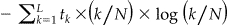where t_k is the number of equivalence classes of size k, L is the size of the largest equivalence class, and N the total number of records in the sample. An equivalence class is defined as a possible value on the quasi-identifiers, for example, “50 year old male” is an equivalence class. We found that entropy computed from sub-samples were very strongly correlated, therefore, they produce similar results as full sample entropy.

MaxCombs. The maximum number of possible different values for the quasi-identifiers. For example, if we have two quasi-identifiers, say, age and gender, and assume that age has 86 possible values and gender has 2 values, 86 × 2 = 172 is the maximum number of different possible combinations of values for these two quasi-identifiers. It is expected that the greater the maximum number of combinations the more uniques will be in a data set. ³¹

We constructed two prediction models, each with a single independent variable: Entropy, or MaxCombs. An examination of the data indicated an obvious logarithmic relationship between each of these variables and the GAPS cut-off, giving us the following two linear models: log (GAPS_CUTOFF) ∼ β₀ + β₁log (Entropy) and log (GAPS_CUTOFF) ∼ β₀ + β₁log (MaxCombs). For each of the two prediction models we had 209 observations representing the quasi-identifier models.

The GAPS cut-off value is truncated from below at 5,000 because that is the smallest subsample that was selected. It is also truncated at the top at 200,000 for central and western Canada, and 60,000 for eastern Canada because that was the size of the total sample that we used. Neither Entropy nor MaxCombs is truncated. A suitable modeling technique for such a censored data set is Tobit regression. ^45–47

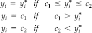
Let y denote the actual value of the GAPS cut-off, the point at which the approximate derivative is close to zero, produced during our simulations. We have y ≥ c ₁ and y ≤ c ₂, where c ₁ and c ₂ are the bottom and top truncation threshold values respectively. Also, let there be an underlying latent variable of which y is the realized observation, such that , where x_i is a matrix with the first column equal to 1 and the second value is the independent variable we are using to predict the GAPS cut-off, β is a vector of parameters, and ɛ_i are independent and normally distributed errors with zero mean and constant variance. The latent variable is the value that we would expect to observe if there was no censoring.

The Tobit model takes the form:

Maximum likelihood estimators were computed using SAS version 9.1 (proc LIFEREG).

To determine the goodness of fit of the models, we used the pseudo-R² of McKelvey and Zavoina, ⁴⁸ which was shown to be valid for the Tobit model. ⁴⁹ A Monte Carlo simulation compared different pseudo-R² measures for the Tobit model and found this one to be the best, ⁵⁰ with the main criterion being equivalence to the R² measure that would be obtained using ordinary least squares regression if there was no censoring in the data.

Validation of GAPS Cut-off Predictions Models

To validate the GAPS cut-off values that we used, the delta score was computed for each of the three regions of Canada. This score indicates how far the uniqueness at the GAPS cut-off was from the asymptotic value. Small values of the delta score indicate that uniqueness is close to zero, and that any additional geographic area aggregation would have an insignificant impact on uniqueness.

An end-user can enter either the Entropy or MaxCombs values in the Tobit models to predict the GAPS cut-off value for their study. To validate the accuracy of the prediction models, we used the Tobit models to predict the GAPS cut-off using 10-fold cross-validation. ^51,52 That is, we divided the data sets into deciles and used one decile in turn for validation, and the remaining nine deciles to build the model.

The predicted cut-off used for validation was the unconditional value of the realized variable y—the full equation for this estimate is provided in the literature. ^45–47 Using y in the validation ensured that the predicted value was also censored. The quality of the prediction was evaluated by considering the median and trimmed mean of the error (y−y) and the relative error, defined as (y−y)/y.

Applying the Prediction Models

Since an end-user does not need to worry about censoring (which is an artifact of our simulation), the predicted value of the latent variable would be used instead, y#x002A;. This is given by y* = e ^β₀ Entropy ^β₁ or yб* = e ^β₀ MaxCombs ^β₁ where β ₀ and β ₁ are the model parameter estimates.

After presenting the results in the next section, the application of the prediction models in several real examples pertaining to the disclosure of retail and hospital pharmacy data to commercial data aggregators is illustrated in the discussion.

Results

An example of the relationship between GAPS and proportion uniqueness is shown in ▶. A similar pattern was observed for all regions and variable combinations. As illustrated in ▶, the cut-off was calculated from such a graph by fitting a model and taking its derivative. The cut-off values were then used to develop the prediction models, as described in the previous section.

Figure 2.

Example showing the actual relationship between geographic area size and proportion uniques in the central region for the three variables: age, gender, and ethnicity.

▶ shows the delta scores, which indicate how far uniqueness was from the asymptotic value at the various GAPS cut-offs that were calculated. As can be seen, there is very little difference in uniqueness across the regions, suggesting that there is little disclosure control benefit in increasing area sizes beyond the cut-offs that were calculated.

Table 2.

Table 2 Table Showing the Delta Scores for the Three Regions. The Delta Score Represents the Proportion of Uniques at the Computed Geographical Area Population Size (GAPS) Cutoff Value. For Example, 0.0036 of the Individuals in Western Canada Were Unique at the GAPS Cutoff (median value)

	West	Central	East
Trimmed mean	0.007	0.0068	0.0061
Median	0.0036	0.0033	0.0037

In ▶ ▶ we show the model parameters and diagnostics to predict the GAPS cut-off as a function of Entropy and MaxCombs, respectively. As is clear, all of the parameters are statistically significant, and the goodness of fit is high.

Table 3.

Table 3 Tobit Model Results for the Three Canadian Regional Models Using Entropy and Validation Accuracy Expressed in Terms of the Prediction Error and Relative Prediction Error

Entropy Prediction Model (Western)
Pseudo-R2		0.89
Intercept		6.3; p < 0.0001
Log (entropy) parameter est.		2.8; p < 0.0001
Prediction error (10-fold)		Relative prediction error (10-fold)
Trimmed mean	−4,433	Trimmed mean	0.012
Median	−1,500	Median	−0.02
Entropy Prediction Model (Central)
Pseudo-R2		0.8
Intercept		6.5; p < 0.0001
Log (entropy) parameter est.		2.6; p < 0.0001
Prediction error (10-fold)		Relative prediction error (10-fold)
Trimmed mean	−1,218	Trimmed mean	−0.015
Median	−7,405	Median	0.019
Entropy Prediction Model (Eastern)
Pseudo-R2		0.9
Intercept		7.0; p < 0.0001
Log (entropy) parameter est.		1.8; p < 0.0001
Prediction error (10-fold)		Relative prediction error (10-fold)
Trimmed mean	−1,284	Trimmed mean	0.0024
Median	−524	Median	−0.019

Table 4.

Table 4 Tobit Model Results Using MaxCombs for the Three Canadian Regions and Validation Accuracy Expressed in Terms of the Prediction Error and Relative Prediction Error

MaxCombs Prediction Model (Western)
Pseudo-R2		0.9
Intercept		7.4; p < 0.0001
Log (MaxCombs) parameter est.		0.4; p < 0.0001
Prediction error (10-fold)		Relative prediction error (10-fold)
Trimmed mean	−2,175	Trimmed mean	−0.012
Median	−1,325	Median	−0.016
MaxCombs Prediction Model (Central)
Pseudo-R2		0.9
Intercept		7.3; p < 0.0001
Log (MaxCombs) parameter est.		0.4; p < 0.0001
Prediction error (10-fold)		Relative prediction error (10-fold)
Trimmed mean	−2,472	Trimmed mean	−0.0002
Median	−1,156	Median	−0.013
MaxCombs Prediction Model (Eastern)
Pseudo-R2		0.9
Intercept		7.6; p < 0.0001
Log (MaxCombs) parameter est.		0.3; p < 0.0001
Prediction error (10-fold)		Relative prediction error (10-fold)
Trimmed mean	−920	Trimmed mean	−0.007
Median	−445	Median	−0.015

For both the Entropy and MaxCombs prediction models, the prediction errors are quite small. While the MaxCombs models have a slightly higher goodness-of-fit than the entropy models, the accuracy of the prediction for both are very similar.

Discussion

The results suggest that the three regional models we have constructed for predicting the GAPS cut-off from both the Entropy and MaxCombs values can be quite accurate. They also make clear that having a single GAPS cut-off would be a serious oversimplification and that the appropriate cut-off is a function of the quasi-identifiers that will be collected and the region of Canada.

Geographic areas that are larger than the GAPS cut-off represent low re-identification risk since they are close to the asymptotic risk value of zero, and there is also no disclosure control benefit in aggregating areas beyond the cut-off.

The prediction accuracy results were similar for MaxCombs and Entropy. One would expect Entropy to perform better given that it represents more information about the data distribution. However, there may be a ceiling effect in that the accuracy for either variable is sufficiently high that it is difficult for Entropy to outperform MaxCombs.

In practice, the MaxCombs value is easier to compute than the Entropy value. It is also possible to compute MaxCombs at the outset of a study during the design phase before any data are collected. We therefore recommend using the MaxCombs results in practice since in terms of accuracy they are very comparable to the Entropy results.

To apply these results an analyst first needs to compute the maximum number of combinations for the quasi-identifiers in the data set. Once this MaxCombs value is determined, the prediction models in ▶ can be used to compute the GAPS cut-off. If the cut-off is deemed too large then the analyst can look at ways to reduce the value of MaxCombs by collapsing or coarsening the response categories. This process can be repeated until the cut-off is sensible for the particular study.

Table 5.

Table 5 Prediction Models to Use for Determining the Smallest Region Size Using MaxCombs

Region of Canada	GAPS Cut-off
Western	1588×MaxCombs0.42
Central	1436×MaxCombs0.43
Eastern	1978×MaxCombs0.304

GAPS = geographical area population size.

Applying the Results

The following disclosure control example is about the re-identification of patients from their prescription records—it illustrates the application of our results. Many retail and hospital pharmacies across Canada provide prescription data to commercial data aggregators (we will refer to these data as “prescription records”). Prescription records are used to produce reports on physician prescription patterns and drug use ⁵³ These reports are then sold primarily to the pharmaceutical industry and government agencies.

In practice, the prescription records provided to commercial data aggregators do not contain directly identifying information about the patients (e.g., patient names and telephone numbers). However, it has been argued that the patient information that is disclosed in such records can still re-identify patients, ^54,55 and that this possible re-identification jeopardizes the confidentiality of Canadians' health information. ⁵⁴

The relevant quasi-identifiers in the prescription record are summarized in ▶. We relied on five sources to construct this table: (1) the Canadian Pharmacists Association (CPhA) Pharmacy Claim Standard which defines all fields in the pharmacy electronic record used for claims adjudication, ⁵⁶ (2) a report provided to us on the variables collected by the data management group at IMS Health Canada Inc, one of the largest commercial data aggregators in Canada, ⁵⁷ (3) the investigation report by the Office of the Information and Privacy Commissioner of Alberta (OIPCA) which listed the 37 fields that are collected by commercial data aggregators, ⁵⁸ (4) the results of a survey of provincial pharmacy regulatory authorities, ⁵⁴ and (5) a specification of the data collected by Brogan Inc from Canadian hospital pharmacies (Brogan is another large commercial data aggregator in Canada). ⁵⁹

Table 6.

Table 6 Fields That can be Used to Re-identify Patients in the Prescription Record According to Our Five Sources. For Hospital Pharmacies Other Data, Such as Dates for Admission and Discharge, are Collected. However, Here We Focus on the Variables That are Common Between Retail and Hospital Pharmacies

Variable	CPhA Standard		IMS 57	Field in OIPCA Report? 58	Disclosed According to Survey? 54	Brogan 59	Additional Explanations
	Defined in CPhA Std? 56	CPhA Mandatory? 56
Patient gender	Y	O	R	Y	Y ∗∗	Y	All sources indicate that patient gender is collected.
Patient year of birth	Y	O	R	Y	Y ∗∗	Y	The survey suggests that some provinces collected the full date of birth. 54 But both the OIPCA report 58 as well as the IMS Health Reports 57 indicate that only the year of birth is collected.
Patient postal code	Y	O	—	—	n ∗∗∗	Y†	The survey indicated that only PEI allowed the collection of postal codes. 54 When we contacted the pharmacy registrar in PEI it was made clear that if geographic information was disclosed by pharmacies, only the FSA was being disclosed rather than the full postal code. The IMS health report indicated that neither the full postal code nor FSA are collected from any province. 57 The Brogan document indicated that the FSA was being collected. 59
Pharmacy postal code	Y	M	Y	Y	—	Y	Brogan's data are from hospital pharmacies, therefore the pharmacist is known.
Prescriber postal code	Y	O	Y ∗	Y	Y¶	Y	Prescriber group is in the record layout for the Brogan data.

^∗ whether this field is collected depends on the arrangement with a particular pharmacy and on the province (not collected in BC, MN, QC).

^∗∗ except MN, QC, NS.

^∗∗∗ except PEI.

^¶ except BC, SK, MN, Nfld.

^† Brogan collects the patient FSA as part of its record layout.

M = Mandatory field in the CPhA claims standard; O = optional field. These fields will not necessarily be available for every pharmacy submitting data; CPhA = Canadian Pharmacists Association; SD = standard deviation; OIPCA = Office of the Information and Privacy Commissioner of Alberta; R = The field is required by IMS health Canada from all pharmacies submitting data, but if it is missing that would not invalidate the record.

The field is not defined or collected at all.

Key variables that are disclosed pertaining directly to patients are gender and year of birth.

Brogan also collects the patient FSA, but IMS Health does not do so directly. However, it is often possible to infer new information about individuals from variables that already exist in a record: ¹¹ it may be possible to infer the patient (residence) postal code from the postal code of their pharmacy or the prescriber if one assumes that there is some regularity in the distances that patients travel to see their general practitioner, specialist, or pharmacist. A simulation concluded that a patient would have to live at most within a 100-m radius from the pharmacy or prescriber to be able to accurately predict the full postal code in urban areas. ¹¹ For rural areas, the distance varies from 1 km in Nova Scotia, 5 km in Ontario, to 10 km in Alberta. ¹¹ We conducted a similar simulation to determine the accuracy of inferring the FSA and concluded that this can be accurately predicted if the patient lives within 10 km of the pharmacist/prescriber for rural areas, and within 1 km for urban areas in Nova Scotia and Alberta, and 0.5 km in Ontario.

In our analysis, we therefore made the assumption that the FSA was being collected or that it was reasonable to accurately infer the FSA for some of the patients if it is not collected.

Example 1

In this example, the prediction models were applied to assess patient re-identification risk for pharmacy prescription records in ten Canadian provinces, for the two quasi-identifiers of age and gender. The MaxCombs value is 172; the number of all possible values of age (86) × gender categories (2). For each of the three regions of Canada the GAPS cut-off was computed using the values in ▶. The percentage of FSAs whose population size is above the predicted cut-off for each province along with the percentage of the population that resides in these FSAs was then calculated.

The results are summarized in ▶, and compared to the three other cut-offs that were being used: the 20,000 cut-off used in HIPAA (in practice the HIPAA Privacy Rule is sometimes used in Canada ⁶⁰ ), the Statistics Canada 70,000 cut-off for the CCHS, and the Census Bureau 100,000 cut-off. These data show that, except for New Brunswick, the vast majority of the provincial populations live in FSAs that are larger than the GAPS cut-off and therefore there is no disclosure control benefit in aggregating the geography any further.

Table 7.

Table 7 The Percentage of FSAs and the Provincial Populations That Would be Above the GAPS Cut-off for an Age × Gender Quasi-identifier Combination for All Ten Canadian Provinces. These Counts are Based on the 2001 Census FSA Population Numbers Provided by Statistics Canada

Province	Our GAPS Models		20,000 Cut-off		70,000 Cut-off		100,000 Cut-off
	FSA	Pop	FSA	Pop	FSA	Pop	FSA	Pop
Alberta	55%	84%	38%	71%	1.4%	5%	0.00	0
British Columbia	68%	87%	46%	70%	1.1%	4.%	0.00	0
Manitoba	59%	88%	39%	68%	0	0	0.00	0
New Brunswick	20%	51%	4.5%	19%	0	0	0.00	0
New found land	55%	83%	30%	62%	0	0	0.00	0
Nova Scotia	47%	82%	16%	43%	0	0	0.00	0
Ontario	69%	91%	49%	76%	1.4%	5%	0.20%	1%
PEI	57%	90%	43%	79%	0	0	0.00	0
Quebec	59%	84%	36%	63%	1%	5%	0.25%	0
Saskatchewan	60%	93%	49%	84%	2%	7%	0.00	2%

FSA = forward station area; GAPS = geographical area population size; PEI = Prince Edward Island.

For commercial data aggregators, there are three possible options:

• 1 Suppress the FSAs that are smaller than the cut-off. For example, in Ontario data from 31% (100–69%) of FSAs would need to be suppressed. These 31% of FSAs represent 9% of the Ontario population.

• 2 Given that sex and gender are collected, determine what level of geographic aggregation would be suitable to avoid suppression of any data.

• 3 The analyst coarsens or collapses the response categories of the quasi-identifiers given that the level of geography is fixed at the FSA.

Suppression of data from small FSAs means that pharmacists would not be permitted to provide that data to the commercial data aggregators. Nevertheless, there would be far less FSA suppression using our models compared to the other cut-offs in current use: our models take into account the characteristics of the variables and calibrate the cut-off. For some provinces, no data would be released at all if some of the other GAPS cut-offs are applied.

For the second option described above, one can aggregate FSAs to the postal region, the first character of the postal code. We found that all postal regions in the ten provinces are above the GAPS cut-off. Therefore, inclusion of the sex and gender variables in the prescription record is possible as long as the geographic detail is at the postal region level, since this level of geography is always higher than the cut-off. The advantage of this option is that no data needs to be suppressed at all; however the disadvantage is that the aggregated geographic unit is quite large.

For the third option described above, it is assumed that the FSA geographic detail needs to be retained—the question then is which one of sex and gender is to be coarsened and the interval for grouping the coarsened age categories. For example, instead of disclosing the age in years, age can be disclosed as part of a 2-year interval, a 5-year interval, or a 10-year interval. The results for such coarsened categories are shown in ▶. As expected the percentage of FSAs that can be disclosed increases as the amount of coarsening increases. However, for smaller provinces, such as New Brunswick, the proportion of the population in large FSAs remains low even with 10-years age intervals. ▶ also shows the effect of coarsening the categories for age in terms of the percentage of the population. With 5-years age intervals, 98% of the Ontario population would be living in regions that are larger than the cut-off.

Table 8.

Table 8 The Percentage of FSAs and the Provincial Populations That Would be Above the GAPS Cut-off for an Age × Gender Quasi-identifier Combination for All Ten Canadian Provinces When the Age Variable is Coarsened to Different Sized Intervals

Province	Original Variables		2-yrs Age Intervals		5-yrs Age Intervals		10-yrs Age Intervals
	FSA	Pop	FSA	Pop	FSA	Pop	FSA	Pop
Alberta	55%	84%	68%	92%	79%	96%	84%	98%
British Columbia	68%	87%	78%	93%	90%	99%	93%	99%
Manitoba	59%	88%	66%	92%	72%	95%	78%	98%
New Brunswick	20%	51%	26%	59%	37%	70%	45%	75%
Newfoundland	55%	83%	70%	91%	79%	95%	88%	98%
Nova Scotia	47%	82%	54%	86%	66%	93%	72%	95%
Ontario	69%	91%	78%	96%	84%	98%	87%	99%
PEI	57%	90%	71%	97%	71%	97%	71%	97%
Quebec	59%	84%	70%	91%	82%	96%	88%	99%
Saskatchewan	60%	93%	69%	97%	69%	97%	71%	98%

FSA = forward station area; GAPS = geographical area population size; PEI = Prince Edward Island.

Example 2

In this example we consider a specific data set from a hospital pharmacy. Records for all prescriptions dispensed from the Children's Hospital of Eastern Ontario pharmacy during the period beginning January 2007 to the end of June 2008 were obtained following institutional ethics approval. In total there were 94,100 records. These represent 10,259 patient visits and 6,902 unique patients.

The MaxCombs value for these data are 54 since the patient ages in years range from 0 to 26. Also, almost all of the patients of the hospital come from Ontario and Quebec. Therefore, we used the Central Canada model from ▶.

The results were that 95% of the patients in the prescription record database reside in FSAs that are larger than the cut-off. However, for pediatric hospital patients it is important to know the age in weeks for patients younger than 1 year. Here, the MaxCombs value is 156, and the result is that 89% of the patients live in FSAs that are larger than the Central Canada cut-off.

Summary

These examples show that using the MaxCombs prediction models given in ▶ provide a straightforward technique to determine the GAPS cut-offs for datasets so the re-identification risk is managed while allowing for an increased amount of data to be available to the health researcher.

Relationship to Other Work

There have been previous descriptive studies of uniqueness in the United States population on basic demographic variables, such as age and gender. ^61,62 However, these studies did not explicitly consider the impact of nested geographic areas and their population size on uniqueness.

We used uniqueness as the measure for re-identification risk. Another common criterion for evaluating re-identification risk is k-anonymity. ^63,64 This criterion considers that non-unique records are also risky. However, even under k-anonymity, unique records are still those with the highest probability of re-identification. Therefore, managing the risk of re-identification from uniques remains an important objective in disclosure control.

Earlier work at the United States Census Bureau evaluated nested geographic areas, and provided the basic methodology for our study. ^29,31 This work did not document a general model that can be applied by individuals outside the bureau and that takes into account the characteristics of the quasi-identifiers, which is what we did in this study.

Limitations

The prediction models we present here should be considered as one element in a toolbox of heuristics that can be used for disclosure control. Some other heuristics have been described in previous work. ^65,66

Although we contend that the ten quasi-identifiers we considered represent basic demographics that are quite common in health research, they will not cover all possible quasi-identifiers that may be used in practice. Thus, our results are limited to the specific variables that we have considered in our analysis.

Conclusions

Data custodians often use general population size cut-offs to determine the level of geographic information to disclose in a data set. For example, the HIPAA Privacy Rule's Safe Harbor list allows the release of the first three digits of the ZIP code only if that area has 20,000 or more individuals living in it. National statistical agencies in the United States, UK, and Canada also use such cut-offs as part of their disclosure control practices. The primary rationale for such cut-offs is that there is no disclosure control benefit for aggregating geographic areas beyond that size.

In this paper we performed an empirical evaluation of such cut-offs using Canadian census data. Our results indicate that the appropriate cut-off depends on characteristics of the variables included in the data set; therefore there is not a single cut-off. We developed and validated models to predict such population size cut-offs for Canada. The model which predicted population cut-offs using the maximum number of possible values in the data set had R² values approaching 0.9, and relative error of prediction less than 0.02 across all regions of Canada. Our prediction models were then applied in a risk assessment of the prescription records that are provided by Canadian pharmacies to commercial data aggregators. This assessment indicated that for most of the Canadian population, that there is no disclosure control benefit to aggregating geography beyond the FSA when releasing patient age and gender.

References

- 1.Platt P, Hendlisz L, Intrator D. Privacy Law in the Private Sector: An Annotation of the Legislation in CanadaCanada Law Book; 2004.
- 2.Willison D, Emerson C, Szala-Meneok K, et al. Access to medical records for research purposes: Varying perceptions across Research Ethics Boards J Med Ethics 2008;34:308-314. [DOI] [PubMed] [Google Scholar]
- 3.Woolf S, Rothemich JR S, Marsland D. Selection bias from requiring patients to give consent to examine data for health services research Arch Fam Med 2000;9:1111-1118. [DOI] [PubMed] [Google Scholar]
- 4.Junghans C, Feder G, Hemingway H, Timmis A, Jones M. Recruiting patients to medical research: Double blind randomised trial of ‘opt-in' versus ‘opt-out' strategies Br Med J 2005;331(7522):940Oct 22; Epub 2005 Sep 12. [DOI] [PMC free article] [PubMed] [Google Scholar]
- 5.Jacobsen S, Xia Z, Campion M, et al. Potential effect of authorization bias on medical records research Mayo Clin Proc 1999;74(4):330-338. [DOI] [PubMed] [Google Scholar]
- 6.Nelson K, Rosa E, Brown J, et al. Do patient consent procedures affect participation rates in health services research? Med Care 2002;40(4):283-288. [DOI] [PubMed] [Google Scholar]
- 7.McKinney P, Jones S, Parslow R, et al. A feasibility study of signed consent for the collection of patient identifiable information for a national paediatric clinical audit database Br Med J 2005;330(7496):877-879Apr 16; Epub 2005 Mar 18. [DOI] [PMC free article] [PubMed] [Google Scholar]
- 8.Tu J, Willison D, Silver F, et al. Impracticability of informed consent in the Registry of the Canadian Stroke Network N Engl J Med 2004;350(14):1414-1421. [DOI] [PubMed] [Google Scholar]
- 9.Armstrong D, Kline-Rogers E, Jani S, et al. Eagle. Potential impact of the HIPAA privacy rule on data collection in a registry of patients with acute coronary syndrome. Arch Intern Med 2005;165:1125-1129. [DOI] [PubMed] [Google Scholar]
- 10.Al-Shahi R, Vousden C, Warlow C. Bias from requiring explicit consent from all participants in observational research: Prospective, population based study Br Med J 2005;331:942. [DOI] [PMC free article] [PubMed] [Google Scholar]
- 11.El Emam K, Jonker E, Sams S, et al. Pan-Canadian de-identification guidelines for Personal health information Available at: http://www.ehealthinformation.ca/documents/OPCReportv11.pdf]. Archived at: http://www.webcitation.org/5Ow1Nko5C]. Accessed: May 18, 2007.
- 12.Boulos M. Towards evidence-based, GIS-driven national spatial health information infrastructure and surveillance services in the United Kingdom Int J Health Geographics 2004;3(1). [DOI] [PMC free article] [PubMed]
- 13.O'Dwyer LA, Burton DL. Potential meets reality: GIS and Public health research in Australia Aust N Z J Pub Health 1998;22(7):819-823. [DOI] [PubMed] [Google Scholar]
- 14.Ricketts TC. Geographic information systems and public health Annu Review Pub Health 2003;24:1-6. [DOI] [PubMed] [Google Scholar]
- 15.Cromley EK. GIS and disease Annu Review Pub Health 2003;24:7-24. [DOI] [PubMed] [Google Scholar]
- 16.Brindley P, Maheswaran R. My favourite software: Geographic information systems J Pub Health Med 2002;24(2):149. [DOI] [PubMed] [Google Scholar]
- 17.Richards TB, Croner CM, Rushton G, Brown CK, Fowler L. Geographic information systems and public health: Mapping the future Pub Health Rep 1999;114:359-373. [DOI] [PMC free article] [PubMed] [Google Scholar]
- 18.Mugge R. Issues in protecting confidentiality in national health statistics Proceedings of the Social Statistics Section, American, Statistical Association. 1983.
- 19.Mackie C, Bradburn N. Improving Access to and Confidentiality of Research Data: Report of a WorkshopNational Academies; 2000.
- 20.Justice Gibson. Mr. Mike Gordon and the Minister of Health and Privacy Commissioner of Canada, Federal Court of Canada, February 27 2008.
- 21.Brownstein J, Cassa C, Mandl K. No place to hide—Reverse identification of patients from published maps N Engl J Med 2006;355(16):1741-1742. [DOI] [PubMed] [Google Scholar]
- 22.Brownstein J, Cassa C, Kohane I, Mandl K. An unsupervised classification method for inferring original case locations from low-resolution disease maps Int J Health Geographics 2006;5(56). [DOI] [PMC free article] [PubMed]
- 23.Curtis A, Mills J, Leitner M. Spatial confidentiality and GIS: Re-Engineering mortality locations from published maps about Hurricane Katrina Int J Health Geographics 2006;5(44). [DOI] [PMC free article] [PubMed]
- 24.Armstrong M, Rushton G, Zimmerman D. Geographically masking health data to preserve confidentiality Stat Med 1999;18:497-525. [DOI] [PubMed] [Google Scholar]
- 25.Zimmerman D, Pavlik C. Quantifying the effects of masking metadata disclosure and multiple releases on the confidentiality of geographically masked health data Geogr Anal 2008;40:52-76. [Google Scholar]
- 26.Fefferman N, O'Neil E, Naumova E. Confidentiality and confidence: Is data aggregation a means to achieve Both? J Pub Health Pol 2005;16:430-449. [DOI] [PubMed] [Google Scholar]
- 27.Willenborg L, Mokken R, Pannekoek J. Microdata and disclosure risks Proceedings of the Annual Research Conference of United States Bureau of the Census. 1990.
- 28.Olson K, Grannis S, Mandl K. Privacy protection versus cluster detection in spatial epidemiology Am J Pub Health 2006;96(11):2002-2008. [DOI] [PMC free article] [PubMed] [Google Scholar]
- 29.Hawala S. Enhancing the “100,000” rule: on the variation of percent of uniques in a microdata sample and the geographic area size identified on the file Proceedings of the Annual Meeting of the American, Statistical Association. 2001.
- 30.Greenberg B, Voshell L. Relating risk of disclosure for microdata and geographic area size Proceedings of the Section on Survey Research Methods, American Statistical Association. 1990.
- 31.Greenberg B, Voshell L. The geographic component of disclosure risk for microdata Bureau of The Census 1990.
- 32.Zayatz L, Massell P, Steel P. Disclosure limitation practices and research at the US Census Bureau Neth Off Statistics 1999;14(Spring):26-29. [Google Scholar]
- 33.Zayatz L. Disclosure Avoidance Practices and Research at the US Census Bureau: An UpdateUnited States Census Bureau; 2005.
- 34.Hawala S. Microdata disclosure protection research and experiences at the US Census Bureau. Proceedings of the Workshop on Microdata, 2003 Available at: http://www.census.gov/srd/sdc/microdataprotection.pdf]. Archived at: http://www.webcitation.org/5b7mPeVPi]. Accessed: September 26, 2008.
- 35.Rudolph B, Shah G, Love D. Small numbers, disclosure risk, security, and reliability issues in web-based data query systems J Pub Health Manag Practice 2006;12(2):176-183. [DOI] [PubMed] [Google Scholar]
- 36.Stoto M. Statistical issues in interactive web-based public health data dissemination systemsRAND Health; 2003.
- 37.Marsh C, Dale A, Skinner C. Safe data versus safe settings: Access to microdata from the British census Int Stat Review 1994;62(1):35-53. [Google Scholar]
- 38.Statistics Canada, Canadian Community. Health survey (CCHS). Cycles 2005;3:1 Public Use Microdata File (PUMF) User Guide. 2006.
- 39.Willenborg L, de Waal T. Statistical Disclosure Control in PracticeSpringer-Verlag; 1996.
- 40.Standards for Privacy of Individually Identifiable Health Information, in Federal Register, Dec 28, 2000 (Volume 65, Number 250). 2000. p. 82,511–82,560.
- 41.El Emam K. Overview of factors affecting the risk of Re-identification in Canada, 2006, Access to Information and Privacy Division, Health Canada.
- 42.Dalenius T. Finding a needle in a haystack or identifying anonymous census records J Off Stat 1986;2(3):329-336. [Google Scholar]
- 43.Bethlehem J, Keller W, Pannekoek J. Disclosure control of microdata J Am Stat Assoc 1990;85(409):38-45. [Google Scholar]
- 44. Statistics Canada. Census public use Microdata file: Individuals file user Documentation. 2001.
- 45.Long S. Regression Models for Categorical and Limited Dependent VariablesSage Publications; 1997.
- 46.Breen R. Regression Models for Censored, Sample-Selected, and Truncated DataSage Publications; 1996.
- 47.Maddala G. Limited-Dependent and Qualitative Variables in EconometricsCambridge University Press; 1983.
- 48.McKelvey R, Zavoina W. A statistical model for the analysis of ordinal level dependent variables J Math Sociol 1975;4:103-120. [Google Scholar]
- 49.Laitila T. A pseudo-R2 measure for limited and qualitative dependent variable models J Econ 1993;56:341-356. [Google Scholar]
- 50.Veall M, Zimmermann K. Goodness of fit measures in the Tobit model Oxf Bull Econ Stat 1994;56(4):485-499. [Google Scholar]
- 51.Cherkassky V, Muller F. Learning from DataWiley; 1998.
- 52.Alpaydin E. Introduction to Machine LearningMIT Press; 2004.
- 53.Kallukaran P, Kagan J. Data mining at IMS health: How we turned a mountain of data into a few information-rich molehills Proceedings of the 24th Annual SAS Users Group International Conference. 1999.
- 54.Zoutman D, Ford B, Bassili A. The confidentiality of patient and physician information on pharmacy prescription records CMAJ 2004;170(5):815-816. [DOI] [PMC free article] [PubMed] [Google Scholar]
- 55.Zoutman D, Ford B, Bassili A. Privacy of pharmacy prescription records (author response) CMAJ 2004;171(7):712. [DOI] [PMC free article] [PubMed] [Google Scholar]
- 56.Canadian Pharmaceutical Association Pharmacy claim standard (version 03). 2006.
- 57.Fineberg A. Information requested for “Re-identification Study”IMS Health Canada; 2006.
- 58.Office of the Information and Privacy Commissioner Order of Alberta. Order H2002-003: Alberta Pharmacies and Pharmacists. 2003.
- 59.Brogan, Inc. MedMap Drug Utilization Program, Program Overview, 2008.
- 60.El Emam K. Data Anonymization practices in clinical research: A descriptive StudyHealth Canada; 2006. Access to Inf and Privacy Division.
- 61.Sweeney L. Uniqueness of simple demographics in the US populationCarnegie Mellon University; 2000. Lab for Int Data Privacy.
- 62.Golle P. Revisiting the uniqueness of simple demographics in the US population Workshop on Privacy in the Electronic Society. 2006.
- 63.Samarati P. Protecting respondents' identities in microdata release IEEE Trans Knowl Data Eng 2001;13(6):1010-1027. [Google Scholar]
- 64.Sweeney L. k-anonymity: A model for protecting privacy Int J Uncertainty, Fuzziness and Knowl-Based Syst 2002;10(5):557-570. [Google Scholar]
- 65.El Emam K, Jabbouri S, Sams S, Drouet Y, Power M. Evaluating common de-identification heuristics for personal health information J Med Internet Res 2006;8(4):e28. [DOI] [PMC free article] [PubMed] [Google Scholar]
- 66.El Emam K. Heuristics for de-identifying health data IEEE Sec Privacy 2008:72-75.