Modulation of temporally coherent brain networks estimated using ICA at rest and during cognitive tasks

Abstract

Brain regions which exhibit temporally coherent fluctuations, have been increasingly studied using functional magnetic resonance imaging (fMRI). Such networks are often identified in the context of an fMRI scan collected during rest (and thus are called “resting state networks”); however, they are also present during (and modulated by) the performance of a cognitive task. In this article, we will refer to such networks as temporally coherent networks (TCNs). Although there is still some debate over the physiological source of these fluctuations, TCNs are being studied in a variety of ways. Recent studies have examined ways TCNs can be used to identify patterns associated with various brain disorders (e.g. schizophrenia, autism or Alzheimer's disease). Independent component analysis (ICA) is one method being used to identify TCNs. ICA is a data driven approach which is especially useful for decomposing activation during complex cognitive tasks where multiple operations occur simultaneously. In this article we review recent TCN studies with emphasis on those that use ICA. We also present new results showing that TCNs are robust, and can be consistently identified at rest and during performance of a cognitive task in healthy individuals and in patients with schizophrenia. In addition, multiple TCNs show temporal and spatial modulation during the cognitive task versus rest. In summary, TCNs show considerable promise as potential imaging biological markers of brain diseases, though each network needs to be studied in more detail. Hum Brain Mapp, 2008. © 2008 Wiley‐Liss, Inc.

INTRODUCTION

Functional magnetic resonance imaging (fMRI) has been used for about 15 years, primarily to extract signal from brain regions which are showing blood oxygen level dependent (BOLD) changes in response to a cognitive task. More recently there has been interest in temporally coherent, but not necessarily task‐driven activity, derived from fMRI data. Early studies performed using correlation of a seed voxel in rapidly sampled echo planar imaging (EPI) fMRI data revealed a significant degree of low frequency correlations with contralateral motor regions [Biswal et al., 1995]. These correlations, also present for visual and auditory cortices, appear to be related to both blood flow and to BOLD activity [Biswal et al., 1997] mostly at lower frequencies [Cordes et al., 2001]. Subsequently it was learned that whole brain data temporally sampled at a much lower rate also showed similar temporally coherent regions [Lowe et al., 1998]. There has been some interest in identifying to what degree these correlations are affected by cognitive tasks and previous work suggests that resting correlation are “not affected by tasks which activate unrelated brain regions” [Arfanakis et al., 2000] although early on Lowe did note that TCN's show modulation correlated with behavior in certain brain regions [Lowe et al., 2000]. More recently, Hampson et al. [ 2006] showed that task performance was positively correlated with connection between two brain regions both at rest and during a task. It remains to be seen to what degree a task actually can be considered to activate only an isolated brain region.

Beyond correlation, multivariate methods based upon independent component analysis (ICA) have also been applied to measure functional connectivity, and have the advantage of not requiring a seed voxel or temporal filtering [McKeown et al., 1998]. ICA was developed to solve problems similar to the “cocktail party” scenario in which individual voices must be resolved from microphone recordings of many people speaking at once [Bell and Sejnowski, 1995]. The algorithm, as applied to fMRI, assumes a set of spatially independent brain networks, each with associated time courses. The model used constrains the fluctuations of each voxel in a given component to have the same time course and thus each component can be considered to reveal a temporally coherent network (TCN).

Since the original observations, there have been multiple studies including manipulations of tasks versus a resting baseline or evaluating changes in the correlations in clinical groups. There is some evidence that the spatial maps reflecting TCNs may be more robust than those estimated during a standard approach based upon the general linear model [Calhoun, in press]. ICA has been used to identify several TCNs which are present in healthy subjects either at rest [Beckmann et al., 2005; Kiviniemi et al., 2003; Van de Ven et al., 2004] or during the performance of a task [Calhoun et al., 2001a, 2002; McKeown et al., 1998]. There has also been interest in using TCNs as biological disease markers, e.g., TCNs have been used to distinguish Alzheimer's disease from healthy aging [Greicius et al., 2004]. Two TCNs have been previously studied in schizophrenia [Bluhm et al., 2007; Calhoun et al., 2004a; Garrity et al., 2007]; one includes bilateral temporal lobe regions, which have previously been used to discriminate healthy controls from patients with schizophrenia [Calhoun et al., 2004a]. A second TCN, one of the most studied, includes regions thought to be engaged when the brain is idle, but whose activity decreases on performance of a cognitive task, and is termed the “default mode network” [McKiernan et al., 2003; Raichle et al., 2001].

The default mode network is believed to participate in an organized, baseline “idling” state of brain function that is diminished during specific goal‐directed behaviors [Raichle et al., 2001]. The default mode network has also been shown to decrease in proportion to task difficulty [McKiernan et al., 2003]. It is proposed that the default mode is involved in attending to internal versus external stimuli and is associated with the stream of consciousness, comprising a free flow of thought while the brain is not engaged in other tasks [Gusnard et al., 2001] however there are alternative explanations as well [Hampson et al., 2006]. We reported recently an approach utilizing both temporal lobe and default mode TCNs to differentiate schizophrenia, bipolar disorder, and healthy controls [Calhoun, in press]. Other than these two TCNs, others have been consistently identified [Beckmann et al., 2005] but not studied in detail. For clinical studies, the extraction of TCNs during task performance has been suggested as a way to constrain a participant's behavior beyond just “resting” and also to stimulate the brain with a task that both patients and controls can perform accurately and which is known to elicit robust brain function differences between the two groups [Calhoun, in press]. However it remains to be seen whether the presence of a task affects the resting state networks in a more pervasive manner. Collection of data during rest in subjects with neuropsychiatric disorders is a useful approach in several regards. First, ill subjects are often unable to perform tasks consistently in the scanner or to fully understand complex instructions. However, at rest, there are no such “task” demands. Second, abnormal task performance often occurs in schizophrenia, due to the cognitive disability associated with the disorder. This is often inevitably confounded with concomitant abnormal brain activation in a “chicken and egg” manner. At rest, when there is no task, this problem can be resolved. Finally, the occurrence of symptoms in the scanner, (for example auditory hallucinations in schizophrenia), is usually thought of as undesirable “noise” during performance of a cognitive task but at rest may actually be contributing useful diagnostic information.

In this work, we attempt to address three key questions. First, we wanted to study how similar TCNs identified during a task were to those identified from resting state data. Second, for networks identified both during a task and at rest, we were interested in assessing to what degree they are modulated spatially and temporally. Finally, we also incorporated a clinical group (patients with schizophrenia) to evaluate whether the same observations regarding task TCNs and resting TCNs held for both patients and controls.

We used ICA to analyze two data sets, one collected during rest and the second during the performance of an auditory oddball task [Kiehl et al., 2005a] collected on the same set of healthy controls and schizophrenia patients. The oddball task is one which both patients and controls can perform well. In addition, one of the most robust functional abnormalities in schizophrenia manifests as a decrease in the temporal lobe amplitude of the “oddball response” in event‐related potential (ERP) data [McCarley et al., 1991]. Similar findings have been shown for fMRI data as well, again particularly in temporal regions [Kiehl and Liddle, 2001]. For each condition we identified the TCNs and then defined paired TCNs by using spatial cross correlation to identify TCNs which were present in both experiments. We evaluated spatial and temporal differences due to the experiment (with and without a task) and differences between patients and controls.

To summarize the results, we identified the same TCNs in both tasks, the only difference being one TCN found to be present in the resting state, but not in the auditory oddball data. In addition, the oddball task modulated multiple TCNs spatially and temporally, some positively and some negatively. Finally, interesting patient versus control differences were identified in several of these networks as well.

METHODS

Participants

Participants consisted of 20 healthy controls, 20 chronic schizophrenia outpatients, all of whom gave written, informed, IRB approved consent at Hartford Hospital and were compensated for their participation. Schizophrenia was diagnosed according to the DSM‐IV TR criteria on the basis of a structured clinical interview administered by a research nurse and review of the medical file [First et al., 1995]. Exclusion criteria included any participants with auditory or visual impairment, mental retardation (full scale IQ < 70), traumatic brain injury with loss of consciousness greater than 15 min, presence or history of any neurological illness. Participants were also excluded if they met criteria for alcohol or drug dependence within the past 6 months or produced a positive (assessed by urine toxicology screen on the day of scanning). Patients were slightly older than controls (SZ age = 39.7 ± 10.1; HC age = 31.2 ± 10.9). All but three patients and one control were right handed. All participants were able to perform the oddball task successfully during practice prior to the scanning session. Healthy participants were free of any DSM‐IV TR Axis I disorder or psychotropic medication.

Experimental Design

All participants were scanned during both an auditory oddball task and while resting. The auditory oddball task (AOD) consists of detecting an infrequent sound within a series of regular and different sounds. The task consisted of two runs of auditory stimuli presented to each participant by a computer stimulus presentation system (VAPP) via insert earphones embedded within 30‐dB sound attenuating MR compatible headphones. The standard stimulus was a 500‐Hz tone, the target stimulus was a 1,000‐Hz tone, and the novel stimuli consisted of nonrepeating random digital noises (e.g., tone sweeps, whistles). The target and novel stimuli each occurred with a probability of 0.10; the standard stimuli occurred with a probability of 0.80. The stimulus duration was 200 ms with a 1,000, 1,500, or 2,000 ms interstimulus interval. All stimuli were presented at ∼80 dB above the standard threshold of hearing. All participants reported that they could hear the stimuli and discriminate them from the background scanner noise. Prior to entry into the scanning room, each participant performed a practice block of 10 trials to ensure understanding of the instructions. The participants were instructed to respond as quickly and accurately as possible with their right index finger every time they heard the target stimulus and not to respond to the nontarget stimuli or the novel stimuli. An MRI compatible fiber‐optic response device (Lightwave Medical, Vancouver, BC) was used to acquire behavioral responses for both tasks. The stimulus paradigm data acquisition techniques and previously found stimulus‐related activation are described more fully elsewhere [Kiehl et al., 2001, 2005a]. Participants also performed a 5‐min resting state scan (REST) and were instructed to rest quietly without falling asleep with their eyes open (eyes were open to avoid the possibility that participants would fall asleep).

Image Acquisition

Scans were acquired at the Olin Neuropsychiatry Research Center at the Institute of Living/Hartford Hospital on a Siemens Allegra 3T dedicated head scanner equipped with 40 mT/m gradients and a standard quadrature head coil. The functional scans were acquired transaxially using gradient‐echo echo‐planar‐imaging with the following parameters (repeat time (TR) = 1.50 s, echo time (TE) = 27 ms, field of view = 24 cm, acquisition matrix = 64 × 64, flip angle = 70°, voxel size = 3.75 × 3.75 × 4 mm³, slice thickness = 4 mm, gap = 1 mm, 29 slices, ascending acquisition). Six “dummy” scans were performed at the beginning to allow for longitudinal equilibrium, after which the paradigm was automatically triggered to start by the scanner. The auditory oddball task consisted of two 8‐min runs and the resting state scan consisted of one 5‐min run.

Preprocessing

Data were preprocessed using the SPM5 software package (http://www.fil.ion.ucl.ac.uk/spm/software/spm5/). Data were motion corrected using INRIalign—a motion correction algorithm unbiased by local signal changes [Freire et al., 2002], spatially normalized into the standard Montreal Neurological Institute space, and spatially smoothed with a 10 × 10 × 10 mm³ full width at half‐maximum Gaussian kernel. For reporting in tabular form, coordinates were converted to the standard space of Talairach and Tournoux [ 1988]. Following spatial normalization, the data (originally acquired at 3.75 × 3.75 × 4 mm³) were slightly subsampled to 3 × 3 × 3 mm³, resulting in 53 × 63 × 46 voxels. Group spatial ICA [Calhoun et al., 2001b] was used to decompose all the data into components using the GIFT software (http://icatb.sourceforge.net/) as follows. Dimension estimation, to determine the number of components, was performed using the minimum description length (MDL) criteria, modified to account for spatial correlation [Li et al., in press]. Note the MDL approach is data driven and hence not dependent upon whether data is collected at rest or during a task. Using this approach, the auditory oddball and the resting data were both estimated to have 19 components. The impact of order selection (estimating the number of components) can have an impact on the number of TCNs identified. In this article, we chose the number of components to match the number estimated using an information theoretic approach [Li et al., in press]. Once the estimate of the number of components was determined we applied ICA to the data using group ICA [Calhoun et al., 2001b] as follows. Data from all subjects were concatenated and this aggregate data set reduced to 19 temporal dimensions using PCA, followed by an independent component estimation using the infomax algorithm [Bell and Sejnowski, 1995].

Creation of Spatial Maps and Time Courses

For each participant, spatial maps were then reconstructed and converted to Z values, hence the intensities of the image provide a relative strength of the degree to which the component contributes to the data [Beckmann et al., 2005]. Each of the 19 components was manually inspected for the presence of obvious artifacts (e.g. edges, ventricles). A final list of 11 components for oddball and 12 components for resting state were then selected for further analysis. It is possible to automatically detect known networks by spatially sorting the components in GIFT using masks derived from the wake forest university pick atlas (http://www.fmri.wfubmc.edu/download.htm) [Correa et al., 2007], however for the purpose of this paper we wanted to ensure finding all relevant TCNs. A voxel‐wise one‐sample t‐test was computed for each group and both components (this treats each subject as a random effect and hence provides a statistical threshold on the maps) [Calhoun et al., 2001b]. Results are shown in Figure 1 and thresholded at P < 0.001 (corrected for multiple comparisons). To compute the degree of task‐relatedness of the brain mode time courses, regressors modeling the target and novel stimuli were created (calculated by convolving the ideal timing of the events with a canonical hemodynamic response function) using the SPM5 software. These regressors were fit to the calibrated time courses for each individual using GIFT and the average percent signal change was computed for each group.

Figure 1.

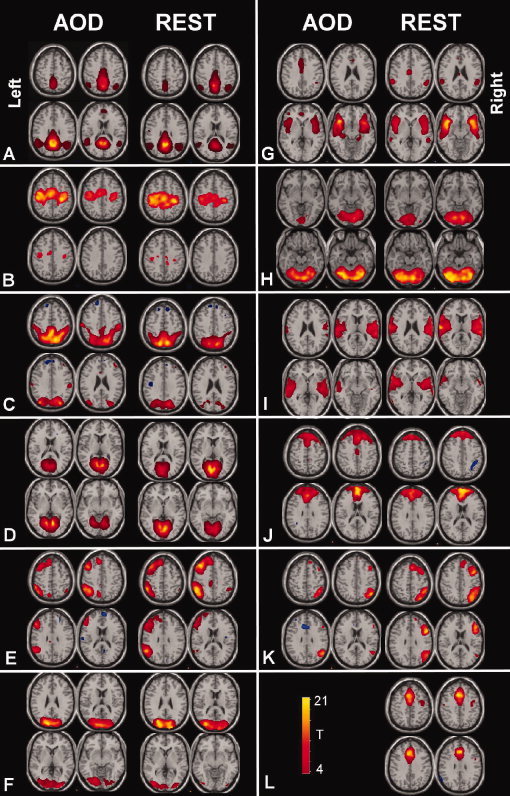
TCNs identified for the auditory oddball task and during the resting state: TCNs identified for AOD (left side of each column) and the most spatially correlated component for REST (right side of each column). Each TCN was entered into a 1‐sample t test and is thresholded at P < 1e‐5 (corrected for multiple comparisions using the family wise error approach implemented in the SPM5 software). Four slices from each TCN are shown.

Comparisons Performed

We compared the auditory oddball TCNs and the resting state TCN both spatially and temporally. A spatial cross‐correlation was used to rank order the spatial similarity of all the TCNs estimated from the two tasks using the TCN maps averaged across all participants. The TCNs which were highly similar were then compared directly for auditory oddball versus resting using a paired t‐test. We also tested for an interaction between auditory oddball versus resting data and patients versus controls. Next, the spectral similarity of the TCN timecourses was determined by computing a binned power spectral density [Garrity et al., 2007]. For each of these measures we also compared differences between patients and controls.

RESULTS

After removing components which showed obviously artifactual patterns or ventricle regions, spatial correlation revealed 11 common TCNs between the two tasks. The TCNs are shown in Figure 1 and spatial cross‐correlation values are shown in Table I. Eight of the 11 TCNs were similar to those identified in previous work [Beckmann et al., 2005]. We give initial labels to the TCNs based upon the regions involved. The identified networks were labeled as follows: (A) default mode network, (B) sensorimotor system, (C) posterior parietal, (D) medial visual areas, (E) left lateral frontoparietal, (F) lateral visual areas, (G) anterior temporal lobe, (H) cerebellum, (I) temporal lobe, (J) medial frontal, (K) right lateral frontoparietal, (L) limbic lobe. One TCN (L) was identified in the resting scan data but did not have a corresponding TCN in the auditory oddball task.

Table I.

Spatial cross‐correlation of TCNs between auditory oddball and resting state data

Comp#		Description	Corr
Oddball	Rest
16	19	A: Default mode	0.9577
11	9	B: Motor	0.9156
13	12	C: Sup parietal	0.9142
10	6	D: Medial visual	0.8628
12	7	E: Left lateral frontoparietal	0.8557
14	2	F: Temporal2	0.8170
17	13	G: Cerebellum	0.8135
8	11	H: Temporal1	0.8059
1	15	I: Frontal	0.8048
4	16	J: Right lateral frontoparietal	0.7838
2	4	K: Lateral visual	0.8170
	5	L: Anterior cingulate	0.0350

Results from the spatial cross‐correlation of the TCNs for auditory oddball and resting data. Eleven TCNs were strongly correlated, one TCN was present in the resting data but not in the auditory oddball data.

For the auditory oddball task, we can utilize the paradigm information to identify the task‐relatedness of each TCN. We used the temporal sorting available in GIFT (http://www.icatb.sourceforge.net), which utilizes a multiple regression fit to each subjects' ICA timecourses (one for each component). Regressors included targets, novels, and standards for both runs as well as their temporal derivatives. Task relatedness can be assessed by performing an analysis of the resulting fit parameters. A TCN is considered task‐related if the regressor parameter fit survives a one‐sample t‐test. Table II shows the T‐values and corresponding p‐values for the target (Tar) and novel (Nov) stimuli (all P‐values are corrected for multiple comparisons using the false discovery rate [FDR]) [Genovese et al., 2002]. We allowed for varying hemodynamic delay by incorporating the temporal derivative term and computed the same measures (not shown), but this did not change the results [Calhoun et al., 2004b]. The last two columns show the patient versus control differences in targets (Tar HC > SZ) and novels (Nov HC > SZ). Significant comparisons are indicated in bold font.

Table II.

Task‐relatedness of auditory oddball TCNs

Description	Tar	Nov	Tar HC > Sz	Nov HC > Sz
A: Default mode	−8.44 (1.4e‐9)	−5.79 (5.6e‐6)	−0.40 (1.0)	−2.87 (3.6e‐2)
B: Motor	4.62 (2.3e‐4)	1.11 (1.0)	−2.43 (1.1 e ‐1)	2.77 (4.6e‐2)
C: Sup parietal	2.51 (8.9e‐2)	−3.50 (6.5e‐3)	−4.51 a (3.2e‐4)	−0.60 (1.0)
D: Medial visual	1.09 (1.0)	0.12 (1.0)	−5.72 a (6.9e‐6)	0.42 (1.0)
E: Left lateral fronto	2.41 (1.1e‐1)	1.21 (1.0)	2.55 (8.1e‐2)	2.33 (1.4e‐1)
F: Temporal2	10.29 (6.2e‐12)	7.76 (1.1e‐8)	5.44 (1.7e‐5)	5.19 (3.7e‐5)
G: Cerebellum	4.09 (1.1e‐3)	−2.59 (7.4e‐2)	2.71 (5.5e‐2)	0.89 (1.0)
H: Temporal1	13.67 (1.2e‐15)	9.30 (1.1e‐10)	1.79 (4.5e‐1)	6.07 (2.3e‐6)
I: Frontal	−2.55 (8.1e‐2)	−3.28 (1.2e‐2)	1.48 (8.1e‐1)	2.53 (8.6e‐2)
J: Right lateral fronto	−12.00 (6.3e‐15)	−3.89 (2.1e‐3)	−0.47 (1.0)	−3.07 (2.1e‐2)
K: Lateral visual	−4.34 (5.4e‐4)	−3.92 (1.9e‐3)	−0.68 (1.0)	1.09 (1.0)

T‐values and corresponding P‐values (in parentheses) for the target (Tar) and novel (Nov) stimuli (FDR corrected for multiple comparisons). The last two columns show the patient versus control differences in targets (Tar HC > SZ) and novels (Nov HC > SZ). Significant comparisons are indicated in bold font.

^aGroup differences were not interpreted because the TCN was not significantly task‐related.

We examined the frequency response of the TCNs during the auditory oddball task and while at rest. For each TCN, we computed a power spectral density (psd). Next, we reduced the psd to six frequency bins to perform comparisons. In this comparison we were specifically interested in testing whether the difference we found previously in patients versus controls in the default mode network during a task was also present at rest or in different TCNs. Specifically we previously found that patients showed significantly more high‐frequency fluctuations and controls showed significantly more low‐frequency fluctuations [Garrity et al., 2007]. Two‐sample t tests were performed on each of the six bins for patients versus controls and results are shown in Table III and Figure 2. Surprisingly, all TCNs for both AOD and REST showed a similar pattern of significantly more low frequency power in controls and significantly more high frequency power in patients.

Table III.

Frequency content of patients versus controls for each TCN

Description	Comp#	Low					High
Oddball
A: Default mode	16	5.63 (1.6E‐06)	1.63 (1.1E‐01)	−5.13 (7.8E‐06)	−6.33 (1.6E‐07)	−5.31 (4.4E‐06)	5.63 (1.6E‐06)
B: Motor	11	4.54 (5.1E‐05)	1.72 (9.3E‐02)	−4.39 (8.1E‐05)	−6.72 (4.6E‐08)	−3.75 (5.6E‐04)	4.54 (5.1E‐05)
C: Sup parietal	13	6.93 (2.3E‐08)	6.07 (3.8E‐07)	−7.32 (6.7E‐09)	−9.4 (1.1E‐11)	−9 (3.7E‐11)	6.93 (2.3E‐08)
D: Medial visual	10	2.7 (1.0E‐02)	8.87 (5.4E‐11)	−3.58 (9.2E‐04)	−4.97 (1.3E‐05)	−5.92 (6.1E‐07)	2.7 (1.0E‐02)
E: Left lateral frontoparietal	12	6.86 (2.9E‐08)	1.06 (3.0E‐01)	−3.47 (1.3E‐03)	−6.6 (6.8E‐08)	−6.73 (4.5E‐08)	6.86 (2.9E‐08)
F: Temporal2	14	6.55 (8.0E‐08)	2.76 (8.7E‐03)	−4.27 (1.2E‐04)	−4.39 (8.1E‐05)	−3.41 (1.5E‐03)	6.55 (8.0E‐08)
G: Cerebellum	17	4.71 (3.0E‐05)	3.39 (1.6E‐03)	−3.98 (2.8E‐04)	−5.87 (7.2E‐07)	−5.84 (7.9E‐07)	4.71 (3.0E‐05)
H: Temporal1	8	6.08 (3.6E‐07)	4.93 (1.5E‐05)	−1.94 (5.9E‐02)	−5.79 (9.3E‐07)	−5.88 (7.0E‐07)	6.08 (3.6E‐07)
I: Frontal	1	5.04 (1.0E‐05)	−3.21 (2.6E‐03)	−5.09 (8.9E‐06)	−7.34 (6.3E‐09)	−4.42 (7.4E‐05)	5.04 (1.0E‐05)
J: Right lateral frontoparietal	4	6.81 (3.5E‐08)	1.96 (5.7E‐02)	−2.94 (5.4E‐03)	−3.78 (5.1E‐04)	−6.76 (4.1E‐08)	6.81 (3.5E‐08)
K: Lateral visual	2	7.86 (1.2E‐09)	3.26 (2.3E‐03)	−4.61 (4.1E‐05)	−8.08 (6.2E‐10)	−6.65 (5.8E‐08)	7.86 (1.2E‐09)
Rest
A: Default mode	19	6.64 (6.0E‐08)	10.51 (4.5E‐13)	−2.69 (1.0E‐02)	−7.42 (4.9E‐09)	−5.66 (1.4E‐06)	6.64 (6.0E‐08)
B: Motor	9	4.97 (1.3E‐05)	−0.62 (5.4E‐01)	−0.93 (3.6E‐01)	−6.77 (3.9E‐08)	−5.03 (1.1E‐05)	4.97 (1.3E‐05)
C: Sup parietal	12	5.85 (7.7E‐07)	2.79 (8.0E‐03)	−5.64 (1.5E‐06)	−6.91 (2.5E‐08)	−7.17 (1.1E‐08)	5.85 (7.7E‐07)
D: Medial visual	6	4.55 (4.9E‐05)	5.13 (7.8E‐06)	1.46 (1.5E‐01)	−5.47 (2.6E‐06)	−5.72 (1.2E‐06)	4.55 (4.9E‐05)
E: Left lateral frontoparietal	7	8.47 (1.8E‐10)	−3.55 (1.0E‐03)	−7.34 (6.3E‐09)	−8.35 (2.7E‐10)	−5.36 (3.7E‐06)	8.47 (1.8E‐10)
F: Temporal2	2	6.16 (2.8E‐07)	2.37 (2.3E‐02)	−4.66 (3.5E‐05)	−8.21 (4.1E‐10)	−5.69 (1.3E‐06)	6.16 (2.8E‐07)
G: Cerebellum	13	3.74 (5.8E‐04)	3.25 (2.3E‐03)	−5.46 (2.7E‐06)	−9.83 (3.2E‐12)	−4.63 (3.8E‐05)	3.74 (5.8E‐04)
H: Temporal1	11	5.4 (3.3E‐06)	2.59 (1.3E‐02)	−3.16 (3.0E‐03)	−6.74 (4.3E‐08)	−6.02 (4.4E‐07)	5.4 (3.3E‐06)
I: Frontal	15	5.14 (7.6E‐06)	−0.55 (5.9E‐01)	−0.39 (7.0E‐01)	−6.98 (2.0E‐08)	−5.02 (1.1E‐05)	5.14 (7.6E‐06)
J: Right lateral frontoparietal	16	4.22 (1.4E‐04)	−0.27 (7.9E‐01)	−2.81 (7.6E‐03)	−4.44 (6.9E‐05)	−3.73 (5.9E‐04)	4.22 (1.4E‐04)
K: Lateral visual	4	5.42 (3.1E‐06)	0.58 (5.7E‐01)	−3.96 (3.0E‐04)	−8.06 (6.6E‐10)	−4.47 (6.3E‐05)	5.42 (3.1E‐06)
L: Anterior cingulate	5	3.91 (3.5E‐04)	−1.72 (9.3E‐02)	−3.57 (9.5E‐04)	−7.5 (3.8E‐09)	−2.16 (3.7E‐02)	3.91 (3.5E‐04)

Results from a two‐sample t‐test for controls versus patients for each of six frequency bins are shown. Paired TCNs for oddball and rest are shown in the same row.

Figure 2.

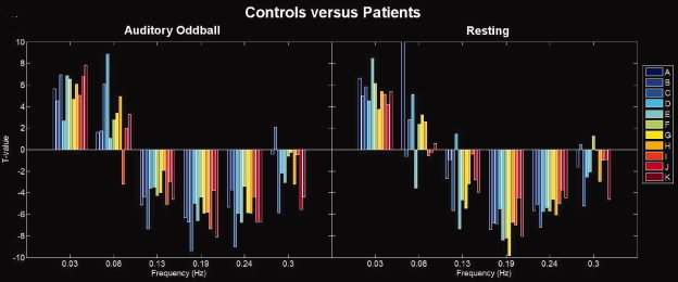
Differences in spectral power for controls versus patients: TCN timecourses for each subject were divided into six frequency bins (the upper range is plotted on the figure, hence the first bin is from [0–0.03 Hz.). For each bin the controls were compared to the patients using a two‐sample t test. Each TCN is plotted in a different color. Positive bars indicate frequency bins where controls are greater than patients, negative bars indicate frequency bins where patients are greater than controls. The overall pattern for all TCNs is that controls show more low frequency power and patients show more high frequency power.

We also determined the degree to which the spatial maps for the TCNs change during rest versus a task, even for those networks which are not showing a strong temporal modulation by the task. We thus performed a paired t test on the spatial maps estimated for the auditory oddball task versus rest and also separately analyzed the patients and controls. Images showing significant differences between AOD and REST, separately for each group, are shown in Figure 3. Surprisingly, we found significant differences between AOD and REST for all of the TCNs and these differences also appeared to change as a function of which group was being compared. The former suggests that there are wide‐spread spatial differences in TCNs during the presence of a task, even for those networks which do not show a strong correlation with the task.

Figure 3.

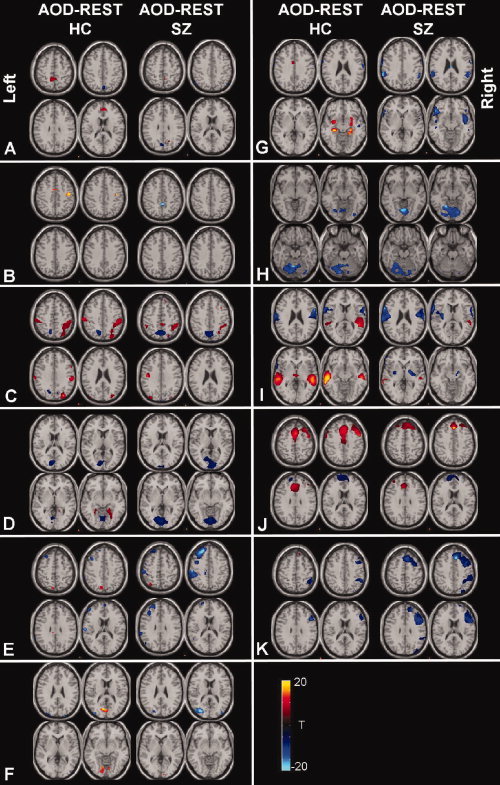
Spatial modulation of TCNs in patients and controls for auditory oddball versus rest: Each paired TCN for AOD and REST were compared by entering the single‐subject spatial maps into a voxelwise two‐sample t test (thresholded at P < 0.05, FDR corrected). Thus for a given voxel a positive value means that the auditory oddball TCN had a larger value at that voxel than the rest TCN. Separate comparisons were performed for healthy controls (left side of each column) and patients (right side of each column).

Figure 3 shows the differences between AOD and REST separately for patients and controls. A direct comparison of the interaction between AOD versus REST and healthy controls versus patients is shown in Figure 4. Regions which changed between AOD and REST but differently for patients and controls were found in several of the TCNs. The largest difference occurred in the first temporal lobe TCN with changes also occurring in the second temporal lobe TCN. For both temporal lobe TCNs controls showed greater temporal modulation by the task than patients. Changes were also observed in the posterior parietal/cingulate TCN, the task‐related right frontoparietal TCN, as well as the medial visual and cerebellar TCNs.

Figure 4.

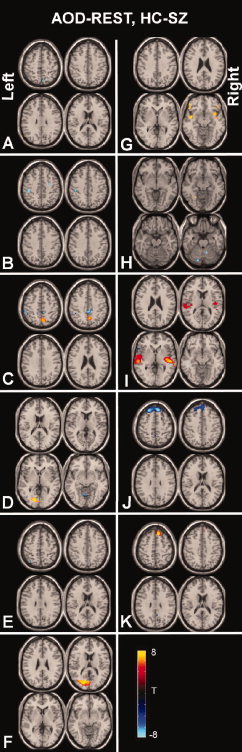
Patient versus control differences between auditory oddball and rest: A direct comparison of patient versus control differences is performed by subtracting each paired TCN for AOD and REST, then entering these into a two‐sample t‐test for patients versus controls (e.g. [(AOD‐REST)_HC−(AOD‐REST)_SZ]). Results are thresholded at P < 0.05 FDR corrected.

DISCUSSION

In this paper we examined TCNs revealed using ICA of fMRI data under two different conditions, during auditory oddball and rest. Results revealed a wide spread pattern of spatial and temporal changes in the TCNs, even for those networks which do not show a significant correlation with the auditory oddball task. This is in contrast to previous work suggesting that TCNs which are not task‐related are not affected by the task [Arfanakis et al., 2000]. In addition, we provide evidence that when using TCNs to study a patient group, an approach which is becoming widely used [Bluhm et al., 2007; Garrity et al., 2007; Greicius et al., 2004; Kiviniemi et al., 2000; Malaspina et al., 2004; Starck et al., 2006], one should also consider the impact that a task has on a TCN.

Results revealed 11 TCNs in common for AOD and REST and one TCN which was present only in REST. Eight of the 11 TCNs were similar to those described in a previous analysis of resting state data [Beckmann et al., 2005]. Of these 11 TCNs, the two temporal lobe networks were strongly related to both targets and novels, and these were the only two networks temporally modulated by the task which showed a difference in temporal modulation between patients and controls (controls showed larger responses than controls). This is consistent with previous work studying the auditory oddball task [Kiehl et al., 2005b]. In addition, the motor and cerebellar networks revealed a significant response only to the targets (consistent with the fact that a button press occurred only in response to target but not to novel stimuli). Two of the TCNs, default mode and right lateral frontal showed strong signal decreases in response to both targets and novels. The lateral visual areas also exhibited signal decreases. The classic default mode component (A) overlaps some with a more frontal component (J) which also shows task‐related decreases. This is interesting and suggests there may be more than one type of “default mode,” further study is warranted. It may also be interesting to explore the relationship of both of these networks with behavior as it is possible that an fMRI signal decrease may also reflect a particular type of engagement [Hampson et al., 2006].

In terms of spectral power, we found a similar pattern across all the TCNs showing higher power in controls at lower frequencies and higher power in patients at higher frequencies. This is consistent with results we reported recently for the default mode network [Garrity et al., 2007]. It is possible that schizophrenia manifests itself in more erratic (higher frequency) communications between brain regions. This is consistent with models of schizophrenia proposing cognitive dysmetria, or impairment of smooth coordination of mental processes and with “disconnection” hypotheses of the disorder [Andreasen et al., 1998]. It was striking to note that this frequency pattern was pervasive across TCNs and also present during both rest and task performance. The relationship between physiologic signals and TCNs is an important ongoing area of research. Some recent studies have attempted to address the issue of possible TCN confounds due to either cardiac or respiratory signals by removing fMRI signal correlated with cardiac or respiration [Birn et al., 2006; Shmueli et al., 2007], but no agreement on a “best approach” yet exists. Complicating the question further is that physiologic signals may be modulated in a top‐down manner via e.g. attention. More work is needed to better understand these issues. Unfortunately we did not measure physiologic information in our data set. However we did evaluate heart rate in a separate sample of chronic schizophrenia patients and healthy controls and found no differences (P = 0.3).

The comparison of AOD and REST reveals that the overall pattern of “activity” in the TCNs is largely consistent. Indeed, at least for the AOD task, no new networks, not present at rest, were identified. However, the spatial comparison of AOD and REST suggests that task performance has a widespread effect on the TCNs, whether they show temporal task‐relatedness or not. This has implications for how one interprets previous results, which typically reports on a particular TCN (e.g. default mode) extracted from a data set collected at rest or during a task. However, when studying subtle effects on each network (such as correlation with some subject‐specific variable), the presence of a task may itself result in a significant difference in the estimated signal. In addition, because the data collected during AOD contains task‐related variance it is difficult to know if the physiologic mechanism behind the patient versus control changes is the same for both paradigms and it may be that the AOD changes are a mixture of two different effects. It will be interesting to investigate aspect in future studies.

Finally, we found significant interactions between AOD versus REST and in patients versus controls. Hence, AOD and REST show small but significant differences in the spatial maps, but these differences are a function of the diagnostic group. That is, TCNs extracted from schizophrenia patients are modulated differently than those extracted from controls. This suggests an additional variable which might prove useful as a disease biomarker. It was also interesting that the data dimensionality was estimated to be the same for both AOD and REST. In future studies it will be interesting to study the estimated data dimensionality at rest and during different tasks in more detail.

In summary, we compared a number of TCNs identified during an auditory oddball task and during rest. Though the overall spatial patterns of each network are preserved, there appear to be widespread statistically significant differences in both AOD versus REST and in patient versus controls.

REFERENCES

- Andreasen NC,Paradiso S,O'Leary DS ( 1998): Cognitive dysmetria as an integrative theory of schizophrenia: A dysfunction in cortical‐subcortical‐cerebellar circuitry? Schizophr Bull 24: 203–218. [DOI] [PubMed] [Google Scholar]
- Arfanakis K,Cordes D,Haughton VM,Moritz CH,Quigley MA,Meyerand ME ( 2000): Combining independent component analysis and correlation analysis to probe interregional connectivity in fMRI task activation datasets. Magn Reson Imaging 18: 921–930. [DOI] [PubMed] [Google Scholar]
- Beckmann CF,de Luca M,Devlin JT,Smith SM ( 2005): Investigations into resting‐state connectivity using Independent Component Analysis. Philos Trans R Soc Lond B Biol Sci 360: 1001–1013. [DOI] [PMC free article] [PubMed] [Google Scholar]
- Bell AJ,Sejnowski TJ ( 1995): An information maximization approach to blind separation and blind deconvolution. Neural Comput 7: 1129–1159. [DOI] [PubMed] [Google Scholar]
- Birn RM,Diamond JB,Smith MA,Bandettini PA ( 2006): Separating respiratory‐variation‐related fluctuations from neuronal‐activity‐related fluctuations in fMRI. Neuroimage 31: 1536–1548. [DOI] [PubMed] [Google Scholar]
- Biswal B,Yetkin FZ,Haughton VM,Hyde JS ( 1995): Functional connectivity in the motor cortex of resting human brain using echo‐planar MRI. Magn Reson Med 34: 537–541. [DOI] [PubMed] [Google Scholar]
- Biswal BB,Van Kylen J,Hyde JS ( 1997): Simultaneous assessment of flow and BOLD signals in resting‐state functional connectivity maps. NMR Biomed 10: 165–170. [DOI] [PubMed] [Google Scholar]
- Bluhm RL,Miller J,Lanius RA,Osuch EA,Boksman K,Neufeld R,Theberge J,Schaefer B,Williamson P ( 2007): Spontaneous low‐frequency fluctuations in the BOLD signal in schizophrenic patients: Anomalies in the default network. Schizophr Bull 33: 1004–1012. [DOI] [PMC free article] [PubMed] [Google Scholar]
- Calhoun VD,Adali T,Pearlson GD,Pekar JJ ( 2001a): Spatial and temporal independent component analysis of functional MRI data containing a pair of task‐related waveforms. Hum Brain Mapp 13: 43–53. [DOI] [PMC free article] [PubMed] [Google Scholar]
- Calhoun VD,Adali T,Pearlson GD,Pekar JJ ( 2001b): A method for making group inferences from functional MRI data using independent component analysis. Hum Brain Mapp 14: 140–151. [DOI] [PMC free article] [PubMed] [Google Scholar]
- Calhoun VD,Pekar JJ,McGinty VB,Adali T,Watson TD,Pearlson GD ( 2002): Different activation dynamics in multiple neural systems during simulated driving. Hum Brain Mapp 16: 158–167. [DOI] [PMC free article] [PubMed] [Google Scholar]
- Calhoun VD,Kiehl KA,Liddle PF,Pearlson GD ( 2004a): Aberrant localization of synchronous hemodynamic activity in auditory cortex reliably characterizes Schizophrenia. Biol Psychiatry 55: 842–849. [DOI] [PMC free article] [PubMed] [Google Scholar]
- Calhoun VD,Stevens M,Pearlson GD,Kiehl KA ( 2004b): FMRI analysis with the general linear model: Removal of latency‐induced amplitude bias by incorporation of hemodynamic derivative terms. NeuroImage 22: 252–257. [DOI] [PubMed] [Google Scholar]
- Calhoun VD,Pearlson GD,Maciejewski P,Kiehl KA: Temporal lobe and default hemodynamic brain modes discriminate between Schizophrenia and Bipolar Disorder. Hum Brain Mapp (in press). [DOI] [PMC free article] [PubMed] [Google Scholar]
- Cordes D,Haughton VM,Arfanakis K,Carew JD,Turski PA,Moritz CH,Quigley MA,Meyerand ME ( 2001): Frequencies contributing to functional connectivity in the cerebral cortex in resting‐state data. AJNR Am J Neuroradiol 22: 1326–1333. [PMC free article] [PubMed] [Google Scholar]
- Correa N,Adali T,Calhoun VD ( 2007): Performance of blind source separation algorithms for fMRI analysis. Magn Reson Imaging 25: 684. [DOI] [PMC free article] [PubMed] [Google Scholar]
- First MB,Spitzer RL,Gibbon M,Williams JBW ( 1995): Structured Clinical Interview for DSM‐IV Axis I Disorders‐Patient Edition (SCID‐I/P,Version 2.0). New York: Biometrics Research Department, New York State Psychiatric Institute. [Google Scholar]
- Freire L,Roche A,Mangin JF ( 2002): What is the best similarity measure for motion correction in fMRI time series? IEEE Trans Med Imaging 21: 470–484. [DOI] [PubMed] [Google Scholar]
- Garrity A,Pearlson GD,McKiernan K,Lloyd D,Kiehl KA,Calhoun VD ( 2007): Aberrant default mode functional connectivity in Schizophrenia. Am J Psychiatry 164: 450–457. [DOI] [PubMed] [Google Scholar]
- Genovese CR,Lazar NA,Nichols T ( 2002): Thresholding of statistical maps in functional neuroimaging using the false discovery rate. Neuroimage 15: 870–878. [DOI] [PubMed] [Google Scholar]
- Greicius MD,Srivastava G,Reiss AL,Menon V ( 2004): Default‐mode network activity distinguishes Alzheimer's disease from healthy aging: Evidence from functional MRI. Proc Natl Acad Sci USA 101: 4637–4642. [DOI] [PMC free article] [PubMed] [Google Scholar]
- Gusnard DA,Akbudak E,Shulman GL,Raichle ME ( 2001): Medial prefrontal cortex and self‐referential mental activity: Relation to a default mode of brain function. Proc Natl Acad Sci USA 98: 4259–4264. [DOI] [PMC free article] [PubMed] [Google Scholar]
- Hampson M,Tokoglu F,Sun Z,Schafer RJ,Skudlarski P,Gore JC,Constable RT ( 2006): Connectivity‐behavior analysis reveals that functional connectivity between left BA39 and Broca's area varies with reading ability. Neuroimage 31: 513–519. [DOI] [PubMed] [Google Scholar]
- Kiehl KA,Liddle PF ( 2001): An event‐related functional magnetic resonance imaging study of an auditory oddball task in schizophrenia. Schizophr Res 48: 159–171. [DOI] [PubMed] [Google Scholar]
- Kiehl KA,Laurens KR,Duty TL,Forster BB,Liddle PF ( 2001): Neural sources involved in auditory target detection and novelty processing: An event‐related fMRI study. Psychophysiology 38: 133–142. [PubMed] [Google Scholar]
- Kiehl KA,Stevens M,Laurens KR,Pearlson GD,Calhoun VD,Liddle PF ( 2005a): An adaptive reflexive processing model of neurocognitive function: Supporting evidence from a large scale (n = 100) fMRI study of an auditory oddball task. NeuroImage 25: 899–915. [DOI] [PubMed] [Google Scholar]
- Kiehl KA,Stevens MC,Celone K,Kurtz M,Krystal JH ( 2005b): Abnormal hemodynamics in Schizophrenia during an auditory oddball task. Biol Psychiatry 57: 1029–1040. [DOI] [PMC free article] [PubMed] [Google Scholar]
- Kiviniemi V,Jauhiainen J,Tervonen O,Paakko E,Oikarinen J,Vainionpaa V,Rantala H,Biswal B ( 2000): Slow vasomotor fluctuation in fMRI of anesthetized child brain. Magn Reson Med 44: 373–378. [DOI] [PubMed] [Google Scholar]
- Kiviniemi V,Kantola JH,Jauhiainen J,Hyvarinen A,Tervonen O ( 2003): Independent component analysis of nondeterministic fMRI signal sources. Neuroimage 19: 253–260. [DOI] [PubMed] [Google Scholar]
- Li Y,Adali T,Calhoun VD: Estimating the number of independent components for fMRI data. Hum Brain Mapp (in press). [DOI] [PMC free article] [PubMed] [Google Scholar]
- Lowe MJ,Mock BJ,Sorenson JA ( 1998): Functional connectivity in single and multislice echoplanar imaging using resting‐state fluctuations. NeuroImage 7: 119–132. [DOI] [PubMed] [Google Scholar]
- Lowe MJ,Dzemidzic M,Lurito JT,Mathews VP,Phillips MD ( 2000): Correlations in low‐frequency BOLD fluctuations reflect cortico‐cortical connections. Neuroimage 12: 582–587. [DOI] [PubMed] [Google Scholar]
- Malaspina D,Harkavy‐Friedman J,Corcoran C,Mujica‐Parodi L,Printz D,Gorman JM,Van HR ( 2004): Resting neural activity distinguishes subgroups of Schizophrenia patients. Biol Psychiatry 56: 931–937. [DOI] [PMC free article] [PubMed] [Google Scholar]
- McCarley RW,Faux SF,Shenton ME,Nestor PG,Adams J ( 1991): Event‐related potentials in Schizophrenia: Their biological and clinical correlates and a new model of Schizophrenic pathophysiology. Schizophr Res 4: 209–231. [DOI] [PubMed] [Google Scholar]
- McKeown MJ,Makeig S,Brown GG,Jung TP,Kindermann SS,Bell AJ,Sejnowski TJ ( 1998): Analysis of fMRI data by blind separation into independent spatial components. Hum Brain Mapp 6: 160–188. [DOI] [PMC free article] [PubMed] [Google Scholar]
- McKiernan KA,Kaufman JN,Kucera‐Thompson J,Binder JR ( 2003): A parametric manipulation of factors affecting task‐induced deactivation in functional neuroimaging. J Cogn Neurosci 15: 394–408. [DOI] [PubMed] [Google Scholar]
- Raichle ME,MacLeod AM,Snyder AZ,Powers WJ,Gusnard DA,Shulman GL ( 2001): A default mode of brain function. Proc Natl Acad Sci USA 98: 676–682. [DOI] [PMC free article] [PubMed] [Google Scholar]
- Shmueli K,van Gelderen P,de Zwart JA,Horovitz SG,Fukunaga M,Jansma JM,Duyn JH ( 2007): Low‐frequency fluctuations in the cardiac rate as a source of variance in the resting‐state fMRI BOLD signal. Neuroimage 38: 306–320. [DOI] [PMC free article] [PubMed] [Google Scholar]
- Starck T,Littow H,Anttola L,Greicius MD,Tervonen O,Isohanni M,Kiviniemi VJ ( 2006): Impaired default‐mode network activity in Schizophrenia: A resting‐state fMRI Study In: Proc. ISMRM, p 530. [Google Scholar]
- Talairach J,Tournoux P ( 1988): A Coplanar Sterotaxic Atlas of a Human Brain. Thieme, Stuttgart: Georg Thieme Verlag. [Google Scholar]
- Van de Ven VG,Formisano E,Prvulovic D,Roeder CH,Linden DE ( 2004): Functional connectivity as revealed by spatial independent component analysis of fMRI measurements during rest. Hum Brain Mapp 22: 165–178. [DOI] [PMC free article] [PubMed] [Google Scholar]