

Abstract
The hydrophobic association of two parallel graphene sheets is studied using the 3D-RISM HNC integral equations with several theoretical methods for the solvent distribution functions. The potential of mean force is calculated to study the effects of the aqueous solvent models and methods on the plates as a function of distance. The results of several integral equations (IE) are compared to MD simulations for the same model. The 3D-IEs are able to qualitatively reproduce the nature of the solvent effects on the potential of mean force but not quantitatively. The local minima in the potential of mean force occur at distances allowing well defined layers of solvent between the plates but are not coincident with those found in simulation of the same potential regardless of the theoretical methods tested here. The dewetting or drying transition between the plates is generally incorrectly dependent on steric effects with these methods even for very hydrophobic systems without solute-solvent attractions, in contradiction with simulation.
I. Introduction
Since the conception and implementation of the three dimensional – reference interaction site model (3D-RISM) integral equation (IE) method, the theory has been applied to large anisotropic models to obtain structural details not possible using the analogous one dimensional theory1-3. The solutions to the IEs are used to predict the thermodynamic properties of the solution as well as the spatial distribution of the solution species4, 5. Studies of the conformational stability of molecular solutes based on thermodynamic considerations have shown the structural stability to depend on a delicate balance between competing forces among the solution species6. This is especially true for biomolecules where the folding mechanism and stability are determined by thermodynamic interactions within and between the solute and solvent which help to direct the folding of the native structure along a converging path7-10.
The phenomenological forces responsible for stabilizing the folded macromolecule and its association with other biomolecules usually include electrostatic interactions, covalent cross-linking and hydrophobic interactions6. Many models of the stability for macromolecules have implicated effective hydrophobic interactions in the interior of the folded structure consisting mainly of constituents of varying hydrophobicity7, 8. The effective interactions between individual hydrophobic moieties are relatively small but the collective effects of these interactions and the consequences of desolvation in large regions in the interior or at an interface provide the stability seen in biomolecules containing a hydrophobic core. The degree to which the 3D-IEs predict these forces for different solution mixtures is somewhat ambiguous and the study of more basic models is warranted to ascertain the qualitative predictions of the theory. These types of studies are needed for two reasons: to gain an understanding of the predictive quality of the present theory, and to provide a path for relevant advancements to the theory.
A great deal of recent work has been applied to understanding the nature of hydrophobic effects at a fundamental level11-16. The nature of the shorter ranged attractions, less than a few molecular diameters, of hydrophobic species has been described with multiple mechanisms over the years17-23. Authors have attributed the nature of the hydrophobic interactions to arise from either a gain of entropy due to release of solvent structured at the hydrophobic interface22, disruption of the H-bonding network of the aqueous solvent21, the entropic cost of forming the cavity with respect to the size of the solvent19, 20, 23, or combinations of these. A more detailed discussion of these theories is given in the recent review by Ball17. Biochemically, hydrophobicity referrers to a variable with a significant range and is not a property which is binary, i.e. on or off as defined by, for instance, a single contact angle criterion.
In addition to these shorter ranged interactions, a much longer less well understood interaction has been observed at length scales up to a few thousand molecular diameters24, 25. Current explanations for such forces include the existence of microscopic bubbles causing a collapse of the inter-solute region24, 26, and an electrostatic mechanism due to an induced dipole-dipole state from the slow reorientation of the polar solvent at the liquid-solid interface27, 28. There are still differences in how different fields of science define hydrophobicity and the hydrophobic effect29. Here we concentrate on nanoscopic plates larger than atoms but still on the nanoscopic scale which have surface areas in the range of protein-protein contacts.
Simulations and theory have generated literature on a variety of solutes with varying hydrophobicity in polar solvents discussing the factors effecting the magnitude, the length scales of the interactions, and the time dependent kinetics15, 16, 30-32. For solutes in close proximity the factors contributing to the crossover from the solvent separated state to the contact states have been extensively studied15, 18, 33. The length scale of the crossover has been shown to be highly dependent on the solute–solvent attractive interactions15, 33. For models with a repulsive or quite weak attractive interaction the inter-solute region has been shown to go through a drying phase at larger distances of two or three solvent diameters33, 34. The region between the solutes becomes depleted of the polar solvent and ultimately collapses through capillary evaporation. This inter-solute collapse following dewetting, whether for hard sphere systems or for systems where dewetting is purely steric, is thermodynamically characterized by a large positive change in entropy due to the solvent being able to recoup some of the translation and rotational entropy due to the region being released to the bulk solvent.
Simulations of models having realistic solute-solvent attractive terms behave qualitatively differently than their purely repulsive models33-35. The state of hydration in the inter-solute regions in simulations has been shown to be highly dependent on a number of factors characterized by the solute properties such as shape and interaction strength. For example, water was shown to exist in a stable one dimensional hydrogen bonded chain in the interior of a carbon nanotube with sufficient attractive solute-solvent interactions but less so with lower attractions36, 37. Other studies with small attractive interaction terms have shown a two dimensional layer of water to be unstable when confined in a hydrophobic region at close contact15, 38, 39. A systematic analysis33 used the calculated potential of mean force as a function of solute-solvent attraction and distance to determine the full range of hydrophobic effects on the association of 2-D sheets of atoms in aqueous solvent. Those authors showed the hydration state corresponding to the PMF at contact depends critically on the potential. They also observed that the stability of the monolayer of water between the plates at a separation consistent with the atomic diameters of the constituents of the plate-water-plate layers is strongly interaction potential strength dependent.
Simulations of solvation effects are considered the most accurate means to study such model systems at the molecular level but they are computationally intensive. Once the solvent structure is determined via the pair distribution functions (PDF) the thermodynamic properties may be calculated. Many less expensive methods exist for such calculations, which vary in their qualitative and quantitative accuracy, but one of the most promising methods which still accounts for the atomistic nature of the solution species is based on integral equations4. Integral equations based on Ornstein-Zernike (OZ) like constructs are attractive as an economical method for calculating the approximate pair distribution functions for the constituents of a solution40-42. The distribution functions predicted by the IEs can be used to describe much of the thermodynamics of the solution mixture but remain inherently approximate. Statistical thermodynamics provides convenient analytical expressions for the solution thermodynamics using the site-site distribution functions43, 44. Some recent advances in IE theory offer more rigor and accuracy but have yet to be extended to aqueous systems41.
Extensions of the traditional one-dimensional (1D) radial methods to three dimensional (3D) grid calculations show promise for the popular interaction site models1-3, 45 to obtain the solute molecule-solvent site pair distribution functions for a solute molecule at infinite dilution. The 3D-RISM theory which is an extension of 1D-RISM theory46, requires the solvent-solvent correlations from a one dimensional, radial theory, and are used on a 3D grid to calculate the solute molecule-solvent site distributions. The distributions obtained from 3D-RISM provide an approximate angular distribution description of the solvent structure around solute molecules compared to the simple radial distribution functions (RDF) from 1D methods.
Some recent applications of the 3D-IEs have focused on elucidating the thermodynamic role the solvent plays on the conformational stability of large biomolecules such as proteins9, 47, 48. These studies considered the origin of the energetic and entropic contributions to the free energy, and confirmed how the entropic part is a significant driving force in protein folding. An insightful discussion by those authors demonstrated the qualitative and quantitative nature of the results based on modern day solvation mechanisms. Other applications include the prediction of the spatial positioning of solvent species throughout possible cavities in the interior of large biomolecules, where cavities are not always accessible during MD simulation time scales and the results may be expected to show ensemble dependence49-51. In principle this is one of the advantages such methods have over molecular dynamics simulations outside of the grand canonical ensemble; they are able to sample all of configuration space where as NVE and NPT MD simulations can suffer from sampling errors due to time constraints.
The IEs and their closures are only approximations and little has been discussed in the literature on the deficiencies of the 3D-IE theory as compared to volumes written on 1D theories compared with other methods (simulation or experiment). Comparison with the same Hamiltonian or potential model used in simulation for a non-pathological system eliminates the ambiguity of comparison with experiment. Once the accuracy of the theory for a given model is known, comparison with experiment can establish the precision of the model with confidence.
Here we address the question as to how accurately 3D-RISM equations describe a particular well studied system of interest, namely the 2D plates considered by this group earlier via simulation[11,30,33,35]. Some of the primary focus is on the dewetting transition seen in the simulation results and how the 3D-IEs coupled with the HNC closure will handle this transition. Expectations are limited since the HNC closure, like many other closures, is incapable of predicting coexisting phases[52]. This is mathematically shown in density functional theory to due with the 2nd order truncation of the expansion in density of the thermodynamic potential and the reality that only a single minimum with respect to density occurs in a quadratic function52. The solvent behavior as described by IEs for small hydrophobic solutes has been studied in numerous papers12, 14, 53-55. The IE approach provides convenient analytical expressions for the solution thermodynamics using the site-site distribution functions43, 44. The IEs in these studies generally provided qualitative descriptions of the solvation of small species. We also wish to quantitatively compare the effect of the solvent-solvent correlations from several IEs on the results for 2D plates. We will quantitatively compare the free energy from IE results for the state of hydration for various models of water near 2D plates of varying hydrophobicity with the exhaustive simulation data.
The IE approach is many orders of magnitude more computationally efficient than simulations, but questions about the accuracy and precision of the numerical solutions are still outstanding5. Numerical solutions for larger solutes which require a larger spatial grid can be difficult to obtain and can exhaust large amounts of memory. The convergence and memory issues are the dominating factors in considering which numerical method to use. Direct inversion of the iterative subspace (DIIS) 56-59 methods are known as being well balanced between memory requirements and convergence of the solutions. However the method is not an exact minimization routine. It is only as good as the solutions being used in its iterative subspace. Methods based on a Newton-Raphson type iterative routine are exact in that they will minimize the residual if the starting solution is within the radius of convergence. The negative aspect of these routines is dealing with a potentially large Jacobian matrix which has to be calculated, stored and inverted60. In this paper we will present a method based on an exact iterative routine which does not require the storage of the full Jacobian or the costly matrix inversion.
In section II of this paper an introduction to the integral equations, the thermodynamic equations and the numerical method used in this study are given. Section III describes the model interactions used in this study and in the corresponding simulation. In section IV the hydration structure and thermodynamics predicted by 3D-IEs is compared with simulation results to show the qualitative nature of the IE methods. Section V contains our conclusion.
II. Theory and Methods
A. Equations
The three-dimensional molecular solute–solvent site distributions were calculated using the 3D-RISM IEs1, 3, 45 for a multi-component fluid using various approximations for the solvent distributions. For a solute molecule at infinite dilution the equation can be expressed as,
| (1) |
where huv(r) is the 3D solute-solvent pair total correlation function, cuv(r) is the 3D solute-solvent direct correlation function, ρ is the particle number density of the solvent, wvv(r) is the intra-molecular correlation function of the solvent, and hvv(r) is the solvent site-site distribution functions which we obtained from and will compare among various theories including RISM46, DRISM61, 62,and closure optimized PISM variants40. The matrix convolution integral in real space is represented by *. The hyper-netted chain (HNC) equation was used in the 3D calculations as a closure. The HNC equation, although not exact, is computational convenient and gives more reliable results for charged and polar species over a broader range of solution species than some other closure relations 63. The HNC equation is defined for each component as,
| (2) |
where t(r) is the indirect correlation function, t(r)=h(r)-c(r), u(r) is the pair potential between the molecular solute and solvent site, and β is the inverse product of the solution temperature and Boltzmann’s constant. We use this in the traditionally renormalized form.
The solvent site-site distributions in eq 1, hvv, constitute a completely separate problem and are solved independently of the 3D calculations. The RISM equation for the solvent-solvent distributions is
| (3) |
where the correlation functions have the same meaning as in eq 1. Solutions based on XRISM theory are obtained from using eq 3 closed with the HNC (eq 2) in renormalized form64-66. For solution mixtures containing charged sites the correct screening due to the solvent is more accurately represented using dielectrically consistent RISM theory (DRISM)61, 67. DRISM theory is similar to RISM theory but an ad hoc bridge term correcting the long range behavior of the solvent is included in the closure. Methods based on RISM are not formally exact in that the graphical expansion of the RISM equations and includes incorrect terms and excludes other correct ones63. The proper interaction site method (PISM) is a formal improvement over RISM and more accurately represents the graphical expression, but generally provides less accurate results68, 69.
The hydration free energy (HFE) was calculated using the Morita-Hiroike HNC formula43, 44 on the 3D grid as,
| (4) |
The chemical potential can be decomposed into its partial molar enthalpic, Δε, and entropic, Δs, parts using
| (5) |
where the entropic part can be calculated by taking the temperature derivative of the chemical potential (eq 6)53. The entropy is calculated using a finite difference method with a temperature step of 5 K.
| (6) |
B. Numerical methods
The correlation functions ultimately must be computed on a grid of sufficient resolution to capture the details of the finest physical length scales defined by the problem. With atomic diameters and bond lengths defined by angstroms, the grid size needs to be a fraction of an angstrom and the extent of the grid must be well beyond the correlation lengths induced by the solute in the solvent. Given an appropriate grid, coarse solutions to eqs 1 and 2 could be calculated using a Newton-Raphson type numerical scheme on a smaller or reduced grid followed by Picard iterations on the full grid to refine the solution to the desired accuracy. Obtaining solutions in this manner however is usually not feasible due to memory constraints and the time required for large matrix inversions56. We have dealt with both of these issues to make these types of algorithms more tractable. The method presented here is an extension of the multigrid idea developed by Gillian70 where a coarse solution is represented by a subset of points on a finer grid. The projection of the fine grid onto the coarse grid represents a significant reduction in the number of points used to describe the major features of the fluid. The coarse grid does not describe all the fine details in the solutions, but can aid in the reduction of the number of Picard iterations needed on the fine grid to refine the solutions. On returning to the coarse grid values are calculated by averaging the functions at points in the fine grid 60.
To reduce the computationally exhaustive task of inverting large matrices we used an iterative routine to approximate solutions for the linear equations. The algorithm we implemented for the solution to the linear equation, Jx=F, where J is the Jacobian matrix, x is our desired solution and F is the residual error, is the GMRes method71. Methods of this type, based on solving Newton’s equations,
are more stable than Picard or relaxation iterations and when implemented correctly accelerate the convergence of the solution72. The Generalized Minimal Residual (GMRes) routine iteratively forms an approximate solution to x using x0+z, where x0 is an initial starting guess and z is the incremental solution in Krylov space. The approximating solution converges to the exact solution x as the Krylov subspace approaches the rank of the transformation matrix A representing the full set of equations. At each iteration a new approximation to x is formed by minimizing the residual norm in the Krylov subspace, Kk = span(v1,Av1, …, Ak-1v1).
The kth iterative solution to x using z is of the form xk = x0 + Vkyk, where z = Vkyk. The matrix Vk consists of k columns, which are the l2-orthonormal basis (v1, v2, …,vk) of the Krylov subspace and yk consists of the coefficients for the basis set. For each iteration the size of the Krylov subspace is increased by one and the basis set coefficients are calculated to minimize the residual norm. This is continued until the residual norm meets some predetermined convergence criterion. The number of operations needed for each iteration is O(n2), where n is the number of grid points. The number of iterations needed to converge to a solution depends on the initial basis set and the predetermined convergence criterion. An advantage to this routine is that the Jacobian matrix does not have to be stored, if one can efficiently generate the elements of the Jacobian (Appendix I). However, the matrix consisting of the l2-orthonormal basis should be stored, and increases linearly in size with the number of iterations. A common variant of the GMRes routine is one that allows restarting. Once the number of basis vectors gets too large, the GMRes routine is restarted with the last approximate solution to x as the new initial starting solution, x0.
C. Numerical Procedure
After situating the solute coordinates in the approximate center of the 3-D grid, the steps used in our implementation are as follows:
Calculate the potential energy interactions between solute sites and solvent grid points.
Guess initial correlation functions.
If necessary perform a few initial Picard iterations.
Decompose correlation functions into their basis set coefficients and their fine displacements.
Calculate the residual vector.
Calculate the Jacobian elements on the coarse grid.
Perform GMRes routine until predetermined convergence criterion is met.
Calculate new basis coefficients.
Check residual vector to determine if another iteration on the coarse grid is needed (if so return to step 4) or to continue to fine grid (next step).
Calculate fine grid values from the basis set representation and the fine displacements.
Use Picard iterations to refine direct correlation, c(r), solution in the fine grid.
Calculate fine grid residual vector fi+1(r). If this value meets our convergence criteria, the solution to the desired error has been obtained.
Numerical methods similar to the one presented here, which are based on the GMRes method, have previously been successfully applied to 1D site-site IEs72, 73. A final thought on these types of numerical routines is that the responsibility of calculating the solution to the desired criterion is up to the fine grid iterations. For solutions to non-stiff problems a coarser grid can be used to decrease the amount of time needed per iteration, and for stiff problems where convergence issues are the main concern more points should be used in the coarse grid.
III. Model
In this study the integral equations described above are used to study the effective interactions between two planar hydrophobic solutes in a polar solvent of H2O. The results are then compared with simulation results for the same model33. The solute and solvent parameters are identical to the simulation study. The pair potential between the sites is modeled with the Lennard-Jones (LJ) plus coulomb potential. The potential for the solute–solvent interactions in this study is calculated using
| (7) |
The subscripts specify the species of the solvent defined on a grid for the 3D calculations. The symbols σ, ε and q are the usual LJ plus Coulomb parameters: the diameter, the well depth and the charge on the atomic sites, respectively. The H2O molecules are represented by the SPC/E model74. The LJ parameters for this SPC/E H2O model have the values of σOO=3.1655 Å, εOO=0.1554 kcal mol-1 and qO=-0.8476 for the sites characterizing the oxygen atom, and σHH=0.4 Å, εHH=0.02 kcal mol-1 and qH=0.4238 for the sites characterizing the hydrogen atoms. The attractive part of the Lennard-Jones potential is excluded for interactions involving the solvent hydrogen atoms as is consistent with previous usage. The two molecular plates are represented by flat graphene sheets of carbon atoms, the same used by Choudhury and Pettitt33. The sheets consisted of 60 carbon atom sites each and measured ~11 × 12 Å. The carbon atoms have been placed in a rigid hexagonal graphite like pattern with distances of 1.4 Å between nearest neighbors. The LJ parameters for the carbon atoms are σCC=3.4 Å, εCC= 0.3598 kJ mol-1 and the sites are uncharged. These parameters represent sp2 carbon atoms from the AMBER 96 force field from the hydrophobic aromatic peptide residues. The Lorentz-Berthelot combination rules, σOC = (σOO+ σCC)/2 and εOC = (εOO εCC)1/2, are used to calculate the LJ parameters for site-site interacts between different species. For some calculations the solute-solvent attractions are turned off by using this same potential with a Week-Chandler-Anderson decomposition5. The number density of the bulk H2O was 0.03334 Å-3 and the temperature is 298.15 K.
The site-site radial distributions for the H2O solvent, hvv, are calculated using XRISM, DRISM and optimized PISM theories40, 61, 66, 67. The results between XRISM and DRISM are quantitatively indistinguishable for the charge free solutes used here (see Fig. 1) so only the distributions from DRISM theory are shown in the results after Fig. 1. The radial solvent-solvent distributions are calculated on a fine grid of 16,364 points over a range of 40 Å (Δr = 0.00244 Å) to minimize errors when transferred to the 3D grids. To limit the errors in the authenticity of the solution and the thermodynamic variables calculated from 3D distributions the calculations are routinely converged to a relative residual error of 10-12. The 3D calculations are performed in a cubic box measuring 40 Å to a side. The fine grid is defined by a linear grid consisting of 1283 points and the coarse grid consisted of 193 points. We note that some poor initial guesses for thermodynamic values not in a stable part of the phase diagram, result in solutions that initially appear to start to converge down to a relative tolerance of 10-3 or 10-4. These solutions then diverge on further attempts to refine them and so are rejected in our work as unphysical unless stable solutions at our most stringent criteria are met.
Figure 1.
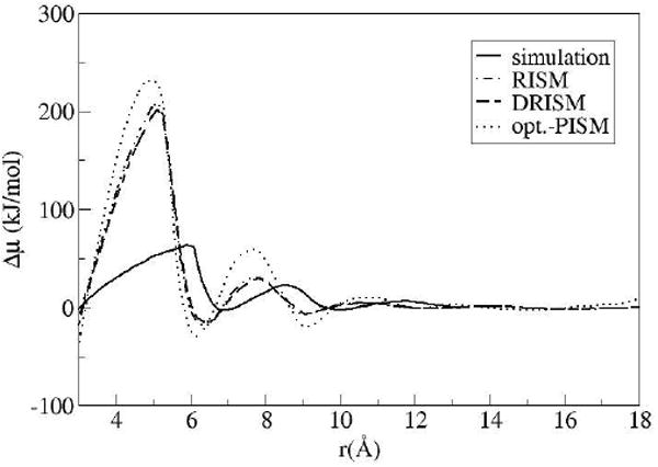
Solvent contributions (HFE) to the PMF for different hvv H2O theories.
IV. Results and Discussion
The 3D distribution functions for the parallel graphene plates in solvent H2O were calculated for inter-solute distances ranging from 1.0–18.4 Å in increments of 0.1 Å. The HNC hydration free energies (HFE) from the 3D-RISM results shown in Figure 1 were calculated using the chemical potential formula44 from eq 4. The value for the infinitely separated plates was subtracted from each curve for each solvent theory. The sensitivity of RISM-like absolute free energies or chemical potentials is well known.
The three sets of data in Figure 1 correspond to the different solvent-solvent distributions obtained from XRISM, DRISM and optimized PISM theory. All of the IE results show qualitative features but are quantitatively disappointing in both the magnitude and phase of the oscillations. As mentioned above, the RISM and DRISM results are similar since graphite has no atomic site charges, so only the DRISM results are displayed throughout the remainder of the analysis. Optimized PISM theory is a recent method for calculating the distribution functions which compares to simulation better than DRISM for pure solvents40. Optimized PISM theory has distributions which are more consistent with the simulation data for the solvent-solvent correlations. However, in this usage it appears to over represent the free energy contributions or features from the solvent when compared to the simulation and DRISM results. It should be mentioned that no separate solute-solvent closure optimization was done here as would be more consistent with that method40.
The HFE contains the contributions to the PMF from direct solvent interactions. The PMF obtained by the addition of the HFE and the direct solute-solute potential is shown in Figure 2 for the DRISM solvent.
Figure 2.
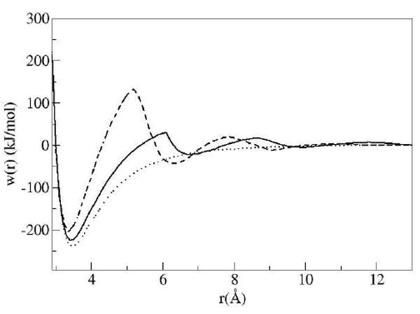
Potential of mean force for DRISM (dashed line) and MD (solid line) results plotted with the direct potential (dotted line) interaction between the plates.
The minimum in the potential of mean force for the solutes in the solute contact configuration (no intervening water layers) predicted by the 3D-RISM theory is 3.4 Å. This distance is ~0.1 Å less than the distance at which the minimum occurred in the PMF obtained from the MD simulation study[33]. Both distances are slightly less than the minimum shown in the direct potential. An explanation for these slightly shorter distances is due to the slope of the cavity potential as the plates are forced together which has been seen in RISM style calculations before75. The generally incorrect placement of the HFE to the direct potential for RISM-like theories has been noted previously and has a variety of consequences for the resulting PMF and properties75.
The PMF shown in Fig 2 for the DRISM solvent has three significant solvent stabilized minima occurring at distances of 6.5, 9.3 and 12.5 Å. These solvent stabilized minima occur at distances allowing well defined solvent layers between the plates as shown in Fig 3 and expected from simulation. The first, second and third solvent separated minima occur at configurations allowing one, two and three intervening water layers between the plates, respectively.
Figure 3.
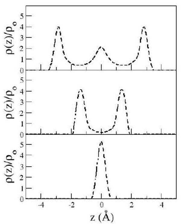
Solute-solvent (oxygen) distributions at the solvent stabilized solute configurations for DRISM at plate separations of 6.5 (bottom), 9.3 (middle), 12.5 (top)
The same characteristics are seen in the results from the simulation study33. However, the simulation results predicted these minima at slightly larger distances consistent with the phase shift in the PMF noted earlier. The DRISM and MD results33 for the solute-solvent oxygen site distributions perpendicular to the plate surfaces for the three minima corresponding to the distances at which the minima occur in the simulations are shown in Figure 4.
Figure 4.
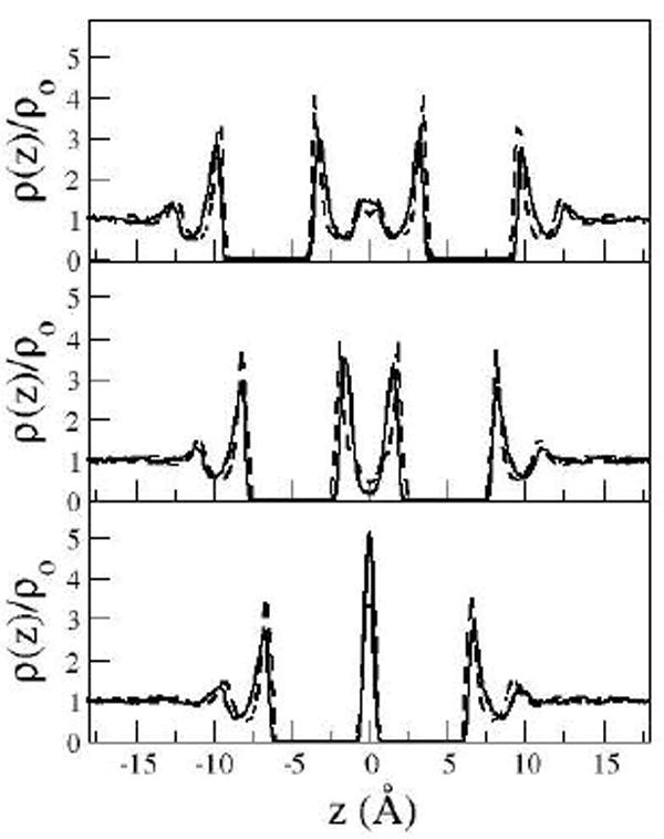
Oxygen site distributions for simulation and DRISM at distances of 6.8 A (bottom), 9.8 (middle), 13 A (top), corresponding the solvent stabilized minima observed in the PMF from simulation.
The distributions shown in Fig 4 from DRISM are structurally similar to the distributions obtained from MD simulations with some noted differences. For the inter-solute distances displayed in Fig 4 all theories predicted well defined peaks for the solvent in contact with the outer surface of the plates. Comparisons with simulation are most favorably made when considering the predicted PMF minima, however the minima are not found at identical distances.
The solvent distributions at the inter-solute distance corresponding to the first solvent separated minimum are characterized by a large single peak between the plates. This represents a well ordered monolayer between the plates. However, this minimum in the PMF for the MD simulation occurs at 6.8 Å which is larger than the DRISM results by about 0.3 Å. The distributions for the second solvent separated minimum are also qualitatively similar between the two methods and represent an ordered bi-layer of water between the plates. The distance between the peaks in the solvent distributions between the plates is 2.9 Å, which roughly corresponds to the peak for O-O distributions of water. However, the inter-plate distance of this feature in the DRISM calculations is about 0.5 Å less than the plate distance from the MD simulation.
There is a third solvent stabilized configuration corresponding to three layers of water between the plates which is also replicated by the IE method. The inconsistency in the locations of the solvent separated minima between IEs and simulation are more pronounced and appear to be due to differences in the effective widths of the solvent structure layers. The structure of the solvent layers for the configurations corresponding to the free energy barriers – the regions between the solvent separated minima – in the PMF are characterized by the expected zig-zag layering of water between the plates, which is also seen in the MD simulations76. The consequence of this layering is a loss of solute-solvent energetic interactions at each surface facing the interior region.
The most prominent characteristic of the PMF from the IEs is the large free energy barrier between the contact state and the first solvent separated state. The IE approach estimates the magnitude of this free energy barrier to be significantly larger than the barrier seen in simulations. The other obvious feature observed in the PMF for both the theories and simulation is a cusp that occurs at the start of the steric drying distance. The solute-solvent interaction energy helps explain the changes occurring in the free energy (Fig 2).
The qualitative energetic features of the solute-solvent interactions in the interior region are reproduced by the 3D-IE theory when compared to MD simulations. As the inter-plate distance decreases from the first solvent separated state the rise in the PMF is mainly attributed to the loss of solute-solvent interactions in the interior region. The cusp in the PMF for MD simulations is sharper because of the well defined, steric-induced loss of these favorable energetic interactions as the monolayer of water is effectively excluded from the interior region. This feature can be seen in Figs 2 and 5 at ~6.0 Å. The cusp is not as sharp in the PMF from the IE theory because the IEs allow some probability of water molecules to remain in sterically forbidden positions located above the center of the hexagonal solute atom configuration (see below).
Figure 5.
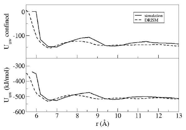
The solute-solvent total potential energy (bottom), and the potential energy between the plates and solvent in the inter-solute region (top) in kJmol-1 for IEs and simulation.
To better understand the factors contributing to the HFE and to investigate the reason for the large free energy barrier in the PMF from IEs, the HFE was separated into its enthalpic and entropic contributions. The partial molar entropy and enthalpy are shown in Figs 6 and 7.
Figure 6.
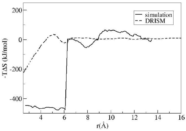
Entropic contribution to the HFE, (-T Δ S)
Figure 7.
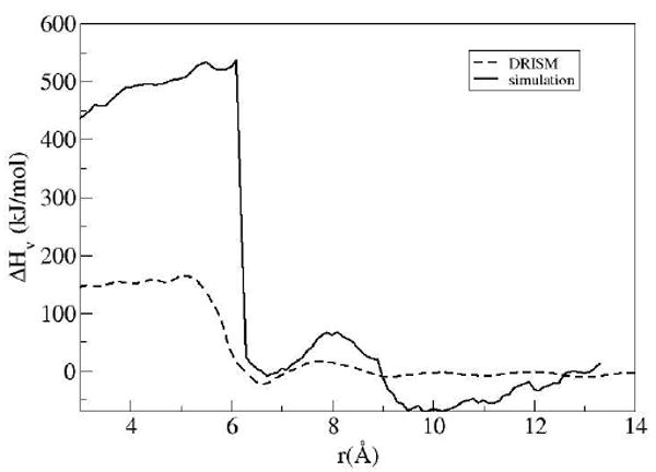
Enthalpic contributions to the HFE, Hv = Δεuv + Δεvv
The nature of the larger free energy barrier is obvious when comparing the factors contributing to the PMF from simulation and IEs. Both methods predict a large positive change in solute-solvent interactions as the solvent is forced from the inter-solute region upon decreasing the plate distance. However, in the simulation result there is a substantial favorable response in the entropy of the solvent which counteracts the energy lost in the solute-solvent interactions. This rapid change in entropy is not seen in the IE results; there is nonetheless a gradual gain in entropy as the inter-solute distance decreases, which is most likely attributed to the gain in translational and rotation entropy as the excluded volume regions overlap or shrink.
As stated earlier, one of the more difficult features of hydrophobic interactions is the length scale at which drying between the plates occurs. In the MD simulations with full solute-solvent interactions33 the smallest inter-plate distance at which water was allowed between the plates is 6.2 Å; any shorter a distance and all the water molecules were excluded due to steric effects. The sharp change in the number of water molecules between the plates was not duplicated by the 3D-IEs with any solvent theory used here. An observation of the distribution functions at these shorter distances shows that there is some nontrivial probability for the water molecules to be located in the sterically forbidden region. Although not explicitly observed by the number of water molecules between the plates, there is evidence that the IEs have a rough qualitative sense of the beginning of the steric drying transition as seen in the MD simulations. For the inter-plate region to be hydrated by water molecules in a hydrogen bonded network forming a two-dimensional sheet ~13 water molecules would be needed to cover the area. The distance at which the number of water molecules falls below 13 in the IEs is about 6.1 Å, as shown in Figure 8, which is near the same length of steric drying in the MD simulations. It is however, unphysically gradual and so the cavity contains significant density when just steric effects would have it be dry.
Figure 8.
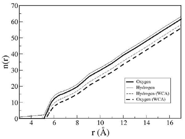
Water oxygen and the sum of hydrogen solvent sites between the plates from DRISM for the model presented and a model represented with the WCA interaction potential.
The number of solvent sites between the plates for a model with no solvent-solute attraction (via the WCA decomposition)77 is also shown in Figure 8. Here we expect to demonstrate the drying effects due to the lack of attraction of the plates. In contradiction to the finding from simulations, the lack of attraction with the IEs does not lead to drying starting at over 10 Å as has been seen and verified by simulation33, 34. In fact the dramatic effect of solute-solvent attractions seen in simulations is effectively suppressed. The lack of a transitional state for the coexistence of phases has been noted before for integral equation methods52. This brings into question the reliability of IEs in situations where a molecular sized cavity might not have sufficient interactions to stabilize a water molecule e.g. on the hydrophobic interior of a protein
Figure 8 also shows the inconsistency in the stoichiometry of the water oxygen and hydrogen sites expected from all XRISM-type theories[63]. Only half the hydrogen site densities are shown so the ratio should be 1:1, but there are consistently more hydrogen atoms between the plates. This behavior continues past the point where all water oxygen sites are excluded from the inter-solute region – the number of hydrogen sites observed should then be zero by stoichiometry. Figure 9 shows the location of the nonzero probability of these rogue hydrogen atoms between the plates. Note that no dissociation is possible for the model and thus this is a pure artifact of the methods.
Figure 9.

Water hydrogen sites between the plates at a separation of 3.0 Å. Shows the existence of finite probabilities of hydrogen between the plates when no oxygens are present, i.e. in carbon-carbon contact.
This stoichiometric problem has been noted for XRISM class theories for some time78. Another property of the solvent in the inter-plate region observed in the MD simulation, which is also computable in the 3D-IE theories, is the orientation of water and the static hydrogen bonding occurring between the plates with a single water layer. The iso-surface plot shown in Fig 10 shows the oxygen atoms (red) tend to occupy the positions directly above the center of the hexagonal pattern. There is both a steric hole as well as an attractive maximum in the potential in these positions.
Figure 10.
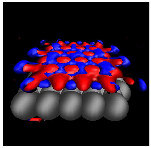
Isosurface of the water oxygen (red) and hydrogen (blue) sites between the plates at a separation of 6.8 Å.
The hydrogen atoms (blue) tend to occupy the positions between the oxygen atoms forming a hydrogen bonding network. The overall orientation of the water molecules is for the plane through HOH to be just above or below the surface of the oxygens which is the same orientational preference observed in MD simulations and in good accord.
Conclusion
In this study we used the 3D-RISM IEs with XRISM, DRISM, and optimized PISM solvent-solvent distributions to calculate the free energies and distribution functions of the solvent water sites around large graphene plates. The graphene sheets were modeled by Lennard-Jones potentials from Amber describing sp2 carbon atom sites with and without the WCA decomposition. The SPC/E water model was used for the solvent. The PMF as a function of inter-plate distance was calculated to determine the ability of the IEs to predict the physical behavior of the solute/solvent combination types presented. The thermodynamic values and structural properties obtained by the IEs were compared to the same from MD simulation results for the same model. The gross structural details of the solvent in contact with the hydrophobic surfaces were consistent between the theories and in reasonable accord with simulation with some notable exceptions. The structural layering of water between the sheets seen in the 3D-IEs was somewhat shifted in position and included stoichiometric deviations compared to the MD simulations.
The free energy barrier for the transition from the first solvent separated configuration to contact was qualitatively replicated by all the IE theories, but was off quantitatively. This barrier was significantly larger for the IE results compared to the MD simulation results. The barrier was shown to be dependent on the expected translation-rotation entropy effects for solvent release (increasing inter-solute distance), and solute-solvent interaction energies for association (decreasing inter-solute distance). The difference in the magnitude of the 1st free energy barrier from IEs and simulations was shown to arise from the inability of the IEs to accurately account for changes in the solvent entropy and the compensating solvent enthalpy when the solvent was excluded from the inter-plate region.
The abrupt change in the number of water molecules between the plates at the transition distance for simulation was not seen by the IE theory and may also reflect the standing controversy in the two-state versus glassy debate for such systems. However, the distance at which the number of water molecules between the plates predicted by the IE theory would not completely hydrate the surface was similar to the distance at which the MD simulations saw dramatic dewetting in the inter-solute region. The IEs were also shown to predict a reasonable orientation of water molecules in contact with the plate surfaces as compared with the MD simulations.
The calculations at high precision shown in this work were done with a combination of Picard/Newton-Raphson based method to obtain the solutions to the 3D-IEs. We showed how the problem of calculating and storing a large Jacobian can be replaced with a method to generate the analytically calculated Jacobian elements as they are needed for a smaller system of equations. Although this numerical method will not completely replace DIIS methods it can help to converge solutions which appear to be unstable with DIIS, especially in the early iterations.
The accuracy of the probability of water in confined spaces and on the interior of macromolecules predicted by this class of theories may suffer from problems found with our more ideal systems. The lack of sharp (first order) hydrophobic drying and inconsistent stoichiometry are problematic. Grand canonical simulations would more accurately quantify this in biomolecule interiors where entrance and escape by diffusion can be problematic.
Acknowledgments
Dr Marcelo Marucho is thanked for the optimized PISM results and many stimulating conversations. This work was supported by the National Institutes of Health (GM066813), the Robert A. Welch Foundation (E-1028), and a training fellowship to JJH from the Keck Center for Computational and Structural Biology of the Gulf Coast Consortia (NLM grant No. 5T15LM07093). BMP thanks Professor Fumio Hirata for a thoughtful discussion on this manuscript.
Appendix 1
To calculate the Jacobian elements we use the following equation, where the 2nd eq is shown in Fourier space and in matrix form.
| (A.1) |
| (A.2) |
The elements of the Jacobian matrix in this implementation are defined as,
| (A.3) |
where the superscripts denote the functions between the solute and the solvent sites, and the subscripts on r denote the position in coordinate space.
The partial derivatives can be calculated using the site-site representation of the HNC closure and the OZ eq in real space. The partial derivative can be calculated as,
| (A.4) |
To calculate the 2nd partial derivative in the last term we start with the OZ equation in momentum space, A.2, and expand into the components for all constituents,
| (A.5) |
Next we can rearrange and collect the constant terms into χba, which is calculated in Fourier space,
| (A.6) |
| (A.7) |
This equation maybe transformed back into real space to give,
| (A.8) |
where the integrals run over all space.
The equation on a discretized grid in Cartesian coordinates, letting r=(x,y,z) and r’=(x’,y’,z’) can be recast as,
| (A.9) |
| (A.10) |
| (A.11) |
for a=b, where i=(x,y,z) and j’=(x’,y’,z’),
| (A.12) |
| (A.13) |
and for a ≠ b
| (A.14) |
| (A.15) |
References
- 1.Beglov D, Roux B. Numerical solution of the hypernetted chain equation for a solute of arbitrary geometry in three dimensions. Journal of Chemical Physics. 1995;103(1):360–4. [Google Scholar]
- 2.Beglov D, Roux B. Integral Equation To Describe the Solvation of Polar Molecules in Liquid Water. Journal of Physical Chemistry B. 1997;101(39):7821–7826. [Google Scholar]
- 3.Cortis CM, Rossky PJ, Friesner RA. A three-dimensional reduction of the Ornstein-Zernike equation for molecular liquids. J Chem Phys. 1997;107(16):6400–6414. [Google Scholar]
- 4.Hirata F. Molecular Theory of Solvation. Vol. 24 Kluwer Academic Publishers; Dordrecht: 2003. [Google Scholar]
- 5.Hansen JP, McDonald IR. Theory of Simple Liquids. Academic Press; San Diego: 1986. [Google Scholar]
- 6.Pace CN, Shirley BA, McNutt M, Gajiwala K. Forces contributing to the conformational stability of proteins. FASEB Journal. 1996;10(1):75–83. doi: 10.1096/fasebj.10.1.8566551. [DOI] [PubMed] [Google Scholar]
- 7.Miranker AD, Dobson CM. Collapse and cooperativity in protein folding. Current Opinion in Structural Biology. 1996;6(1):31–42. doi: 10.1016/s0959-440x(96)80092-3. [DOI] [PubMed] [Google Scholar]
- 8.Itzhaki LS, Evans PA, Dobson CM, Radford SE. Tertiary Interactions in the Folding Pathway of Hen Lysozyme: Kinetic Studies Using Fluorescent Probes. Biochemistry. 1994;33(17):5212–20. doi: 10.1021/bi00183a026. [DOI] [PubMed] [Google Scholar]
- 9.Imai T, Harano Y, Kinoshita M, Kovalenko A, Hirata F. Theoretical analysis on changes in thermodynamic quantities upon protein folding: Essential role of hydration. Journal of Chemical Physics. 2007;126(22):225102/1–225102/9. doi: 10.1063/1.2743962. [DOI] [PubMed] [Google Scholar]
- 10.Onuchic JN, Wolynes PG. Theory of protein folding. Current Opinion in Structural Biology. 2004;14(1):70–75. doi: 10.1016/j.sbi.2004.01.009. [DOI] [PubMed] [Google Scholar]
- 11.Choudhury N, Pettitt BM. The Dewetting Transition and The Hydrophobic Effect. Journal of the American Chemical Society. 2007;129(15):4847–4852. doi: 10.1021/ja069242a. [DOI] [PMC free article] [PubMed] [Google Scholar]
- 12.Lum K, Chandler D, Weeks JD. Hydrophobicity at Small and Large Length Scales. Journal of Physical Chemistry B. 1999;103(22):4570–4577. [Google Scholar]
- 13.Pratt LR, Pohorille A. Hydrophobic Effects and Modeling of Biophysical Aqueous Solution Interfaces. Chemical Reviews (Washington, DC, United States) 2002;102(8):2671–2691. doi: 10.1021/cr000692+. [DOI] [PubMed] [Google Scholar]
- 14.Moghaddam MS, Chan HS. Pressure and temperature dependence of hydrophobic hydration: Volumetric, compressibility, and thermodynamic signatures. Journal of Chemical Physics. 2007;126(11):114507/1–114507/15. doi: 10.1063/1.2539179. [DOI] [PubMed] [Google Scholar]
- 15.Giovambattista N, Rossky PJ, Debenedetti PG. Effect of pressure on the phase behavior and structure of water confined between nanoscale hydrophobic and hydrophilic plates. Physical Review E: Statistical, Nonlinear, and Soft Matter Physics. 2006;73(41):041604/1–041604/14. doi: 10.1103/PhysRevE.73.041604. [DOI] [PubMed] [Google Scholar]
- 16.Huang DM, Chandler D. Temperature and length scale dependence of hydrophobic effects and their possible implications for protein folding. Proceedings of the National Academy of Sciences of the United States of America. 2000;97(15):8324–8327. doi: 10.1073/pnas.120176397. [DOI] [PMC free article] [PubMed] [Google Scholar]
- 17.Ball P. Water as an Active Constituent in Cell Biology. Chemical Reviews (Washington, DC, United States) 2008;108(1):74–108. doi: 10.1021/cr068037a. [DOI] [PubMed] [Google Scholar]
- 18.Pratt LR, Chandler D. Theory of the hydrophobic effect. Journal of Chemical Physics. 1977;67(8):3683–704. [Google Scholar]
- 19.Lee B. Solvent reorganization contribution to the transfer thermodynamics of small nonpolar molecules. Biopolymers. 1991;31(8):993–1008. doi: 10.1002/bip.360310809. [DOI] [PubMed] [Google Scholar]
- 20.Lee B. The physical origin of the low solubility of nonpolar solutes in water. Biopolymers FIELD Full Journal Title:Biopolymers. 1985;24(5):813–23. doi: 10.1002/bip.360240507. [DOI] [PubMed] [Google Scholar]
- 21.Blokzijl W, Engberts JBFN. Hydrophobic effects: opinion and fact. Angewandte Chemie. 1993;105(11):1610–48. (See also Angew Chem, Int Ed Engl. 1993;32(11):1545–79.)
- 22.Frank HS, Evans MW. Free volume and entropy in condensed systems. III. Entropy in binary liquid mixtures; partial molal entropy in dilute solutions; structure and thermodynamics in aqueous electrolytes. Journal of Chemical Physics. 1945;13:507–32. [Google Scholar]
- 23.Lucas M. Size effect in transfer of nonpolar solutes from gas or solvent to another solvent with a view on hydrophobic behavior. Journal of Physical Chemistry. 1976;80(4):359–62. [Google Scholar]
- 24.Parker JL, Claesson PM, Attard P. Bubbles, cavities, and the long-ranged attraction between hydrophobic surfaces. Journal of Physical Chemistry. 1994;98(34):8468–80. [Google Scholar]
- 25.Wood J, Sharma R. How Long Is the Long-Range Hydrophobic Attraction? Langmuir. 1995;11(12):4797–802. [Google Scholar]
- 26.Attard P. Bridging Bubbles between Hydrophobic Surfaces. Langmuir. 1996;12(6):1693–5. [Google Scholar]
- 27.Despa F, Berry RS. The origin of long-range attraction between hydrophobes in water. Biophysical Journal. 2007;92(2):373–378. doi: 10.1529/biophysj.106.087023. [DOI] [PMC free article] [PubMed] [Google Scholar]
- 28.Despa F, Fernandez A, Berry RS. Dielectric Modulation of Biological Water. Physical Review Letters. 2004;93(22):228104/1–228104/4. doi: 10.1103/PhysRevLett.93.228104. [DOI] [PubMed] [Google Scholar]
- 29.Maibaum L, Chandler D. Segue between Favorable and Unfavorable Solvation. Journal of Physical Chemistry B. 2007;111(30):9025–9030. doi: 10.1021/jp072266z. [DOI] [PubMed] [Google Scholar]
- 30.Choudhury N, Pettitt BM. Dynamics of Water Trapped between Hydrophobic Solutes. Journal of Physical Chemistry B. 2005;109(13):6422–6429. doi: 10.1021/jp045439i. [DOI] [PubMed] [Google Scholar]
- 31.Pratt LR. Molecular theory of hydrophobic effects: \“she is too mean to have her name repeated.\”. Annual Review of Physical Chemistry. 2002;53:409–436. doi: 10.1146/annurev.physchem.53.090401.093500. [DOI] [PubMed] [Google Scholar]
- 32.Walther JH, Jaffe R, Halicioglu T, Koumoutsakos P. Carbon nanotubes in water: Structural characteristics and energetics. Journal of Physical Chemistry B. 2001;105(41):9980–9987. [Google Scholar]
- 33.Choudhury N, Pettitt BM. On the Mechanism of Hydrophobic Association of Nanoscopic Solutes. Journal of the American Chemical Society. 2005;127(10):3556–3567. doi: 10.1021/ja0441817. [DOI] [PubMed] [Google Scholar]
- 34.Huang X, Margulis CJ, Berne BJ. Dewetting-induced collapse of hydrophobic particles. Proceedings of the National Academy of Sciences. 2003;100(21):11953–11958. doi: 10.1073/pnas.1934837100. [DOI] [PMC free article] [PubMed] [Google Scholar]
- 35.Choudhury N, Pettitt BM. Enthalpy-Entropy Contributions to the Potential of Mean Force of Nanoscopic Hydrophobic Solutes. Journal of Physical Chemistry B. 2006;110(16):8459–8463. doi: 10.1021/jp056909r. [DOI] [PMC free article] [PubMed] [Google Scholar]
- 36.Hummer G, Rasalah JC, Noworyta JP. Water conduction through the hydrophobic channel of a carbon nanotube. Nature (London, United Kingdom) 2001;414(6860):188–190. doi: 10.1038/35102535. [DOI] [PubMed] [Google Scholar]
- 37.Sansom MSP, Biggin PC. Biophysics: Water at the nanoscale. Nature (London, United Kingdom) 2001;414(6860):156–157. 159. doi: 10.1038/35102651. [DOI] [PubMed] [Google Scholar]
- 38.Wallqvist A, Berne BJ. Computer Simulation of Hydrophobic Hydration Forces on Stacked Plates at Short Range. Journal of Physical Chemistry. 1995;99(9):2893–9. [Google Scholar]
- 39.Wallqvist A, Gallicchio E, Levy RM. A Model for Studying Drying at Hydrophobic Interfaces: Structural and Thermodynamic Properties. J Phys Chem B. 2001;105(28):6745–6753. [Google Scholar]
- 40.Marucho M, Montgomery Pettitt B. Optimized theory for simple and molecular fluids. Journal of Chemical Physics. 2007;126(12):124107/1–124107/9. doi: 10.1063/1.2711205. [DOI] [PMC free article] [PubMed] [Google Scholar]
- 41.Dyer KM, Perkyns JS, Pettitt BM. A site-renormalized molecular fluid theory. Journal of Chemical Physics. 2007;127(19):194506/1–194506/14. doi: 10.1063/1.2785188. [DOI] [PMC free article] [PubMed] [Google Scholar]
- 42.Dyer KM, Perkyns JS, Pettitt BM. Effective density terms in proper integral equations. Journal of Chemical Physics. 2005;123(20):204512/1–204512/11. doi: 10.1063/1.2116987. [DOI] [PMC free article] [PubMed] [Google Scholar]
- 43.Morita T, Hiroike K. A New Approach to the Theory of Classical Fluids. III. Progress of Theoretical Physics. 1961;25(4):537–578. [Google Scholar]
- 44.Singer SJ, Chandler D. Free energy functions in the extended RISM approximation. Molecular Physics. 1985;55(3):621–5. [Google Scholar]
- 45.Kovalenko A, Hirata F. Three-dimensional density profiles of water in contact with a solute of arbitrary shape: a RISM approach. Chemical Physics Letters. 1998;290(123):237–244. [Google Scholar]
- 46.Chandler D, Andersen HC. Optimized cluster expansions for classical fluids. II. Theory of molecular liquids. Journal of Chemical Physics. 1972;57(5):1930–7. [Google Scholar]
- 47.Phongphanphanee S, Yoshida N, Hirata F. On the Proton Exclusion of Aquaporins: A Statistical Mechanics Study. Journal of the American Chemical Society. 2008;130(5):1540–1541. doi: 10.1021/ja077087+. [DOI] [PubMed] [Google Scholar]
- 48.Imai T, Harano Y, Kinoshita M, Kovalenko A, Hirata F. A theoretical analysis on hydration thermodynamics of proteins. Journal of Chemical Physics. 2006;125(2):024911/1–024911/7. doi: 10.1063/1.2213980. [DOI] [PubMed] [Google Scholar]
- 49.Yoshida N, Phongphanphanee S, Maruyama Y, Imai T, Hirata F. Selective Ion-Binding by Protein Probed with the 3D-RISM Theory. Journal of the American Chemical Society. 2006;128(37):12042–12043. doi: 10.1021/ja0633262. [DOI] [PubMed] [Google Scholar]
- 50.Imai T, Hiraoka R, Kovalenko A, Hirata F. Locating Missing Water Molecules in Protein Cavities by the Three-Dimensional Reference Interaction Site Model Theory of Molecular Solvation. Wiley InterScience. 2006;66:804–813. doi: 10.1002/prot.21311. [DOI] [PubMed] [Google Scholar]
- 51.Imai T, Hiraoka R, Kovalenko A, Hirata F. Water Molecules in a Protein Cavity Detected by a Statistical-Mechanical Theory. Journal of the American Chemical Society. 2005;127(44):15334–15335. doi: 10.1021/ja054434b. [DOI] [PubMed] [Google Scholar]
- 52.Evans R. Density functionals in the Theory of Nonuniform Fluids. In: Henderson D, editor. Fundamentals of Inhomogenous Fluids. Marcel Dekker, Inc.; New York: 1992. pp. 85–176. [Google Scholar]
- 53.Pettitt BM, Rossky PJ. Alkali halides in water: ion-solvent correlations and ion-ion potentials of mean force at infinite dilution. Journal of Chemical Physics. 1986;84(10):5836–44. [Google Scholar]
- 54.Akiyama R, Karino Y, Hagiwara Y, Kinoshita M. Remarkable solvent effects on depletion interaction in crowding media: analyses using the integral equation theories. Journal of the Physical Society of Japan. 2006;75(6):064804/1–064804/7. [Google Scholar]
- 55.Pratt LR, Chandler D. Hydrophobic solvation of nonspherical solutes. Journal of Chemical Physics. 1980;73(7):3430–3. [Google Scholar]
- 56.Kovalenko A, Ten-No S, Hirata F. Solution of three-dimensional reference interaction site model and hypernetted chain equations for simple point charge water by modified method of direct inversion in iterative subspace. Journal of Computational Chemistry. 1999;20(9):928–936. [Google Scholar]
- 57.Hamilton TP, Pulay P. Direct inversion in the iterative subspace (DIIS) optimization of open-shell, excited-state, and small multiconfiguration SCF wave functions. Journal of Chemical Physics. 1986;84(10):5728–34. [Google Scholar]
- 58.Pulay P. Improved SCF convergence acceleration. Journal of Computational Chemistry. 1982;3(4):556–60. [Google Scholar]
- 59.Pulay P. Convergence acceleration of iterative sequences. The case of SCF iteration. Chemical Physics Letters. 1980;73(2):393–8. [Google Scholar]
- 60.Kelley CT. Solving Nonlinear Equations with Newton’s Method. Society for Industrial and Applied Mathematics; Philadelphia: 2003. p. 118. [Google Scholar]
- 61.Perkyns J, Pettitt BM. A site-site theory for finite concentration saline solutions. Journal of Chemical Physics. 1992;97(10):7656–7666. [Google Scholar]
- 62.Perkyns J, Pettitt BM. A dielectrically consistent interaction site theory for solvent-electrolyte mixtures. Chemical Physics Letters. 1992;190(6):626–630. [Google Scholar]
- 63.Hansen JP, McDonald IR. Theory of Simple Liquids. Academic; London: 1976. [Google Scholar]
- 64.Hirata F, Pettitt BM, Rossky PJ. Application of an extended RISM equation to dipolar and quadrupolar fluids. Journal of Chemical Physics. 1982;77(1):509–20. [Google Scholar]
- 65.Pettitt BM, Rossky PJ. Integral equation predictions of liquid state structure for waterlike intermolecular potentials. Journal of Chemical Physics. 1982;77(3):1451–7. [Google Scholar]
- 66.Hirata F, Rossky PJ. An extended RISM equation for molecular polar fluids. Chemical Physics Letters. 1981;83(2):329–34. [Google Scholar]
- 67.Perkyns JS, Pettitt BM. A dielectrically consistent interaction-site theory for solvent-electrolyte mixtures. Chemical Physics Letters. 1992;190(6):626–30. [Google Scholar]
- 68.Chandler D, Silbey R, Ladanyi BM. New and proper integral equations for site-site equilibrium correlations in molecular fluids. Molecular Physics. 1982;46(6):1335–45. [Google Scholar]
- 69.Rossky PJ, Chiles RA. A complete integral equation formulation in the interaction site formalism. Molecular Physics. 1984;51(3):661–74. [Google Scholar]
- 70.Gillan MJ. A new method of solving the liquid structure integral equations. Molecular Physics. 1979;38(6):1781–1794. [Google Scholar]
- 71.Saad Y, Schultz MH. GMRES: A Generalized Minimal Residual Algorithm for Solving Nonsymmetric Linear Systems. SIAM J SCI STAT COMPUT. 1986;7(3):856–869. [Google Scholar]
- 72.Booth MJ, Schlijper AG, Scales LE, Haymet ADJ. Efficient solution of liquid state integral equations using the Newton-GMRES algorithm. Computer Physics Communications. 1999;119(23):122–134. [Google Scholar]
- 73.Kelley CT. A fast multilevel algorithm for integral equations. SIAM J Numer Anal. 1995;32(2):501–513. [Google Scholar]
- 74.Berendsen HJC, Grigera JR, Straatsma TP. The missing term in effective pair potentials. Journal of Physical Chemistry. 1987;91(24):6269–71. [Google Scholar]
- 75.Dang LX, Pettitt BM, Rossky PJ. On the correlation between like ion pairs in water. Journal of Chemical Physics. 1992;96(5):4046–7. [Google Scholar]
- 76.Lee CY, McCammon JA, Rossky PJ. The structure of liquid water at an extended hydrophobic surface. Journal of Chemical Physics. 1984;80(9):4448–55. [Google Scholar]
- 77.Chandler D, Weeks JD, Andersen HC. Van der Waals picture of liquids, solids, and phase transformations. Science (Washington, DC, United States) 1983;220(4599):787–94. doi: 10.1126/science.220.4599.787. [DOI] [PubMed] [Google Scholar]
- 78.Hirata F, Rossky PJ, Pettitt BM. The interionic potential of mean force in a molecular polar solvent from an extended RISM equation. Journal of Chemical Physics. 1983;78(6 Pt 2):4133–44. [Google Scholar]