Information-Processing Architectures in Multidimensional Classification: A Validation Test of the Systems Factorial Technology

Abstract

A growing methodology, known as the systems factorial technology (SFT), is being developed to diagnose the types of information-processing architectures (serial, parallel, or coactive) and stopping rules (exhaustive or self-terminating) that operate in tasks of multidimensional perception. Whereas most previous applications of SFT have been in domains of simple detection and visual–memory search, this research extends the applications to foundational issues in multidimensional classification. Experiments are conducted in which subjects are required to classify objects into a conjunctive-rule category structure. In one case the stimuli vary along highly separable dimensions, whereas in another case they vary along integral dimensions. For the separable-dimension stimuli, the SFT methodology revealed a serial or parallel architecture with an exhaustive stopping rule. By contrast, for the integral-dimension stimuli, the SFT methodology provided clear evidence of coactivation. The research provides a validation of the SFT in the domain of classification and adds to the list of converging operations for distinguishing between separable-dimension and integral-dimension interactions.

A fundamental issue in the psychology of perception concerns how information from multiple dimensions is processed in tasks such as detection, recognition, and classification (e.g., Ashby, 1992; Garner, 1974; Kantowitz, 1974; Lockhead, 1972; Schweickert, 1992; Sternberg, 1969; Townsend, 1984). Consider, for example, a simple detection paradigm in which there is a potential target in the left visual field and one in the right visual field. On each trial, the observer's task is to simply detect whether one of the targets is present. One basic question is whether the processing of the information operates in serial fashion or in parallel fashion. In serial processing, information from each visual field is gathered sequentially, one field at a time. By contrast, in parallel processing, information from both visual fields is gathered simultaneously. A second question is whether the processing is exhaustive or self-terminating. In the self-terminating case, processing would stop as soon as a single target is detected. By contrast, in the exhaustive case, processing would continue until the information has been gathered from both visual fields, regardless of whether a target had already been detected in one of them. A third question of interest in the present research is whether the processing may be coactive. In the present example, the intuition is that information from the separate visual fields may summate or be pooled into a common channel prior to an eventual decision-making stage (Colonius & Townsend, 1997; Diederich & Colonius, 1991; Miller, 1982; Townsend & Nozawa, 1995). This summed perceptual information may lead to more efficient decisions than if separate decisions are made for each individual field.

A growing methodology, known as the systems factorial technology (SFT), is being developed to diagnose the type of processing architecture that underlies performance in tasks of multidimensional perception, for example, whether processing is serial or parallel, exhaustive or self-terminating, and whether coactivation has occurred (e.g., Egeth & Dagenbach, 1991; Schweickert, 1985; Schweickert, Giorgini, & Dzhafarov, 2000; Townsend & Ashby, 1983; Townsend & Nozawa, 1995; Townsend & Wenger, 2004a).¹ For the most part, however, applications of the SFT have taken place in the context of simple detection and visual- and memory-search paradigms. One purpose of the present research was to extend the applications of SFT to multidimensional perceptual classification (cf. Fific, 2006; Thomas, 2006; Wenger & Townsend, 2001). In classification, the task is not to determine the presence or absence of targets. Rather, stimulus information is always present, and the task is to use the presented information to classify objects into categories.

An equally important goal of the present research was to use the classification paradigm to provide validation tests of the SFT methodology, particularly with regard to foundational issues in multidimensional perception. A fundamental distinction in multidimensional perceptual classification involves the contrast between integral and separable dimensions (Ashby & Maddox, 1994; Garner, 1974; Shepard, 1964). Integral dimensions are those that combine into relatively unanalyzable, unitary wholes. Examples are colors varying along dimensions of brightness, saturation, and hue. There is extensive converging evidence that observers process such stimuli in holistic fashion. Such evidence leads to the hypothesis that classification decision making for integral-dimension stimuli involves coactive processing of the dimensions. Our reasoning is that in the case of integral-dimension stimuli, the perceptual system apparently glues the individual dimensions into whole objects at an early stage of processing. Thus, rather than the information-processing system making decisions along separate channels, it seems more natural to conceive of the system as operating on a pooled, coactive source of perceptual evidence.

By contrast, separable dimensions are those that remain psychologically distinct when in combination. Examples of stimuli composed of separable dimensions are geometric forms that vary in their shape and in their color. For highly separable-dimension stimuli, it seems far less likely that coactive processing of the individual dimensions takes place. The key question that we pursued in the present research was whether the SFT methodology would reveal the signatures of the expected processing architectures for integral-dimension and separable-dimension stimuli in our classification experiments.

We believe that this goal of providing validation tests for the SFT in the domain of multidimensional perceptual classification is a highly significant one. First, note that much of the previous evidence for the integral-separable processing distinction comes from the results of Garner's (1974) well-known speeded classification tasks. In these tasks, subjects are required to name the level of a single component of a multidimensional stimulus. In the filtering task, the level of a second irrelevant dimension varies orthogonally across trials, whereas in the correlated task, the second dimension provides redundant information. For integral-dimension stimuli, one observes interference in response times (RTs) in the filtering task but facilitation in RTs in the correlated task (compared with a control condition in which the second dimension is held fixed across trials). By contrast, for separable-dimension stimuli, there is no interference in the filtering task and no facilitation in the correlated task. As noted by Ashby and Maddox (1994), although these speeded classification tests have a good deal of intuitive appeal, the resulting integral-separable distinction is only operationally defined. It is only recently that rigorous theoretical explanations have been sought for the empirical pattern of results in these tasks (e.g., Ashby & Maddox, 1994; Nosofsky & Palmeri, 1997a). The present applications of the SFT join in this effort to seek firm theoretical foundations for the integral-separable distinction by testing whether distinct mental-processing architectures are involved.

Second, in our view, the search for converging operations and validation methods is the sign of a maturing science. The SFT has thus far been applied mainly in stimulus-detection and visual–memory search domains, whereas the hypothesis that the classification of integral-dimension stimuli involves coactive processing of the dimensions was derived from independent sources of evidence. In our view, if the present validation tests succeed, they would provide strong converging evidence in favor of the SFT and for past theorizing involving the integral-separable distinction. Given such converging evidence and validation, the SFT could then be applied with even greater confidence to investigate more open-ended issues in perceptual classification. For example, Fific (2006) has initiated investigations with the SFT to determine whether the perceptual classification of face stimuli involves coactivation of individual features and whether such coactive processing may develop with extended practice in the task.

In the remainder of this article, we first briefly review the SFT as applied in the domain of simple detection. We then extend it to the domain of multidimensional classification and proceed to describing the validation tests.

SFT

Applications of SFT make use of the double-factorial paradigm (Townsend & Nozawa, 1995). Using stimulus detection as an example, we illustrate the structure of the paradigm in Figure 1. The stimuli vary along two dimensions. In our detection example, Dimension 1 might correspond to the left visual field, and Dimension 2 might correspond to the right visual field. In the present example, we will suppose that the task is to detect whether a target is present in either field. As illustrated in the figure, on each trial, there may be no target present in either field, a target present in one field but not in the other, or a target present in both fields.

Figure 1.

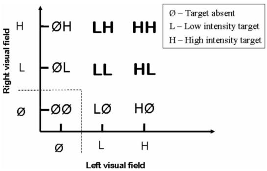
Schematic illustration of the double factorial paradigm in the domain of visual detection. Boldface symbols denote cases in which targets are present in both visual fields.

A key aspect of the paradigm is that a second variable, say the brightness of the targets, is manipulated factorially in each visual field. So, for example, a target that is present in the left visual field may be of either low or high intensity and likewise for a target that is present in the right visual field. It is assumed that the manipulations of light intensity “selectively influence” the processing of the targets in each field (e.g., Dzhafarov, 1999; Schweickert et al., 2000; Sternberg, 1969; Townsend, 1984; Townsend & Schweickert, 1989; Townsend & Thomas, 1994), with faster and more efficient processing of high-intensity targets than low-intensity targets. The selective-influence assumption means that increasing the light intensity in, say, the left visual field increases the processing rate in the left field but would not influence the processing rate in the right visual field.

Mean Interaction Contrasts

For present purposes, the key data of interest involve the trials in which both targets are present. As illustrated in Figure 1, there are four possible target combinations: LL, LH, HL, and HH (where L refers to low intensity and H refers to high intensity). We denote the mean RT for responding to each combination as RT(LL), RT(LH), RT(HL), and RT(HH), respectively. Again, assuming that high intensity leads to faster responding than does low intensity in each separate field, there are three main candidate patterns of mean RTs that one might observe. These patterns are illustrated schematically in Figure 2. The patterns have in common that HH trials lead to the fastest RTs, LH and HL trials lead to intermediate RTs, and LL trials lead to the slowest RTs.

Figure 2.

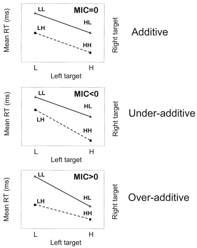
Schematic illustration of three main patterns of mean response times (RTs) and mean interaction contrasts (MICs). L = low-intensity target; H = high-intensity target.

The mean RT patterns illustrated in Figure 2 can be summarized in terms of an expression known as the mean interaction contrast (MIC):

$$\begin{array}{cc}\hfill \mathrm{MIC}=& [\mathrm{RT}\left(\mathrm{LL}\right)-\mathrm{RT}\left(\mathrm{LH}\right)]-[\mathrm{RT}\left(\mathrm{HL}\right)-\mathrm{RT}\left(\mathrm{HH}\right)]\hfill \\ \hfill & =\mathrm{RT}\left(\mathrm{LL}\right)-\mathrm{RT}\left(\mathrm{LH}\right)-\mathrm{RT}\left(\mathrm{HL}\right)+\mathrm{RT}\left(\mathrm{HH}\right).\hfill \end{array}$$

Note that the MIC simply computes the difference between the vertical distance between the leftmost points on each line, RT(LL) – RT(LH), and the vertical distance between the rightmost points on each line, RT(HL) – RT(HH). It is straightforward to see that the pattern of additivity (see Figure 2) is reflected by an MIC value equal to zero. Likewise, underadditivity is reflected by MIC < 0(a negative MIC), and overadditivity is reflected by MIC > 0 (a positive MIC).

Under quite general assumptions, the patterns of additivity, underadditivity, and overadditivity provide important clues concerning the processing architecture and stopping rules that underlie detection performance. The key results are summarized in Table 1. Formal proofs of the results (together with statements of more detailed technical assumptions) are provided by Townsend and Nozawa (1995). Here we provide only a brief review along with informal, intuitive explanations.

Table 1.

Summary of Mean and Survivor Interaction Contrast Predictions for Some Alternative Information-Processing Architectures and Stopping Rules

Architecture	Stopping rule	MIC	SIC(t)
Serial	Self-terminating	0, Additive	Zero (flat)
Serial	Exhaustive	0, Additive	Negative → Positive
Parallel	Self-terminating	>0, Overadditive	Positive
Parallel	Exhaustive	<0, Underadditive	Negative
Coactive		>0, Overadditive	Negative → Positive

Note. MIC = mean interaction contrast; SIC = survivor interaction contrast; t = time units.

If processing is strictly serial, then regardless of whether a self-terminating or exhaustive stopping rule is used, the MIC value will equal zero (i.e., the pattern of mean RTs will show additivity). The intuition here is straightforward. For example, for serial-exhaustive processing, LH trials will show some slowing relative to HH trials due to slower processing of the target in the left visual field. Likewise, HL trials will show some slowing relative to HH trials due to slower processing in the right visual field. If processing is serial exhaustive, then the increase in mean RTs for LL trials relative to HH trials will simply be the sum of the two individual sources of slowing, resulting in the pattern of additivity that is illustrated in Figure 2.

As indicated in Table 1, parallel exhaustive processing will result in a pattern of underadditivity of the mean RTs (MIC < 0). If processing is parallel exhaustive, then processing of both targets will occur simultaneously; however, a final response will not be provided until detection decisions have been made for both visual fields. Thus, the RT will be determined by the slower (i.e., maximum time) of the two individual detection decisions. Clearly, LH and HL trials will lead to slower mean RTs than will HH trials, because processing will tend to be slower if either visual field has a low-intensity target, leading to a slower final response. LL trials will lead to the slowest mean RTs of all, because the more opportunities for an individual detection decision to be slow, the slower on average the final response. The intuition, however, is that detection responses for the individual visual fields begin to run out of room for further slowing. That is, although the RT distributions are unbounded, once one channel has been slowed the probability of sampling a still slower response on the second channel diminishes. Thus, one observes the underadditive increase in mean RTs in this parallel exhaustive case.

Finally, both parallel self-terminating processing and coactive processing will lead to a pattern of overadditivity of the mean RTs (MIC > 0). For example, for parallel self-terminating processing, the speed of the final response will be determined by the faster (i.e., minimum time) of the two individual detection decisions.² Thus, if either visual field has a high-intensity target, responding will tend to be fast, because the decision maker does not need to wait for a potentially slow detection process to complete. Therefore, although LH and HL trials will tend to be somewhat slower on average than will HH trials, the overall slowing will not be very pronounced. By contrast, for LL trials, neither individual detection response will tend to be fast. Thus, the slowing for LL trials will be quite pronounced, leading to the pattern of overadditivity (MIC > 0) that is illustrated in Figure 2. A similar intuition can be developed for the case of coactive processing.³

SICs

Although results involving the MIC already provide important clues as to the processing architecture, this approach has limits in terms of its diagnosticity. For example, the MIC does not distinguish between the cases of serial exhaustive and serial self-terminating processing nor does it distinguish between the cases of parallel self-terminating processing and coactive processing (see Table 1).

More diagnostic power is provided when RTs are examined at the full distribution level. The survivor function, S, for a random variable T (which, in the present case, corresponds to the time of processing) is defined as the probability that the process T takes greater than t time units to complete, S(t) = p(T > t). Note that, for time-based random variables, when t = 0, it is the case that S(t) = 1; and as t approaches infinity, it is the case that S(t) approaches 0. Slower processing is associated with greater values of the survivor function across the time domain.

In a manner analogous to the mean RTs, one can compute the survivor functions associated with each of the four main types of target combinations, which we will denote S_LL(t), S_LH(t), S_HL(t), and S_HH(t). Naturally, because processing is presumably slower for low-intensity targets than for high-intensity targets, the survivor function for LL targets will tend to be of the highest magnitude, the survivor functions for LH and HL targets will tend to be of intermediate magnitude, and the survivor function for HH targets will be of the lowest magnitude. A schematic illustration is provided in Figure 3.

Figure 3.

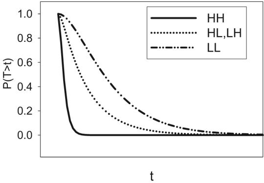
Schematic illustration of the expected ordering of survivor functions associated with each of the four main types of target combinations (HH, HL, LH, and LL). L = low-intensity target; H = high-intensity target; T = time of processing; t = time units.

The precise quantitative relations among the four survivor functions provide diagnostic information concerning the underlying processing architecture. In a manner analogous to the MIC, one can compute the quantity known as the survivor interaction contrast (SIC). Specifically, at each value of t, one computes

$$\begin{array}{cc}\hfill \mathrm{SIC}\left(t\right)=[S_{\mathrm{LL}}\left(t\right)-S_{\mathrm{LH}}\left(t\right)]& -[S_{\mathrm{HL}}\left(t\right)-S_{\mathrm{HH}}\left(t\right)]\hfill \\ \hfill & =S_{\mathrm{LL}}\left(t\right)-S_{\mathrm{LH}}\left(t\right)-S_{\mathrm{HL}}\left(t\right)+S_{\mathrm{HH}}\left(t\right)\hfill \end{array}$$

As illustrated in Figure 4 (and summarized in Table 1), the different processing architectures under consideration yield distinct predictions of the form of the SIC function. There is a close relation with the results from the MIC, because the value of the MIC is simply the integral of the SIC.⁴ However, the SIC also yields more fine-grained information. It would require extensive discussion to develop intuitions for the mathematical derivations of the predicted form of the SIC functions and so here we simply summarize the bottom-line results.

Figure 4.

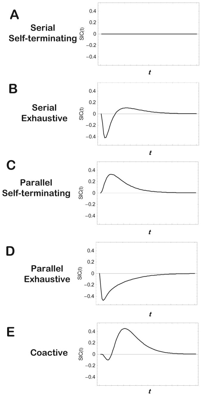
Schematic illustration of the survivor interaction contrast (SIC) functions associated with the different processing architectures and stopping rules. t = time units.

For serial self-terminating processing, the value of the SIC is equal to zero at all time values t (see Figure 4A). If processing is serial exhaustive, the SIC is negative at early values of t but positive thereafter, with the total area spanned by the negative portion of the function equal to the total area spanned by the positive portion (see Figure 4B). Note that for both the serial self-terminating and serial exhaustive cases, the integral of the SIC function (i.e., the MIC) is equal to zero (i.e., the case of mean RT additivity).

If processing is parallel self-terminating, then the value of the SIC is positive at all values of t (see Figure 4C). The integral of the SIC in this case is positive, corresponding to a pattern of mean RT overadditivity. By contrast, for parallel exhaustive processing, the SIC is negative at all values of t (see Figure 4D). The negative integral corresponds to the pattern of mean RT underadditivity.

Finally, for present research purposes, the most critical case involves the signature for coactive processing (see Figure 4E). In this case, the SIC shows a small negative blip at early values of t but then shifts to being strongly positive thereafter. The predicted pattern of overadditivity in the mean RTs is the same as for parallel self-terminating processing, but these two processing architectures are now sharply distinguished in terms of the form of their predicted SIC functions.

Making Provision for Error Responses

The formal results for the MIC and SIC that we have summarized are based on mathematical derivations that assume error-free processing of the multidimensional information. However, on the basis of simulation work that we have conducted, in which the component processes of the mental architectures are represented in terms of random-walk models that give rise to errors, we find that the pattern of predictions is robust (see also Townsend & Wenger, 2004b). We provide a presentation of this simulation work in Appendix A. In a nutshell, the simulations indicate that the serial and parallel architectures yield the expected MIC and SIC signatures even when error rates are very high (e.g., >.30 for the LL stimulus). The coactive architecture yields the expected MIC and SIC signatures for low and moderate error rates. However, depending on detailed parametric assumptions, the predicted pattern of overadditive RTs sometimes disappears when error rates are very high (i.e., >.30 for the LL stimulus). Our ultimate goal is to develop and test detailed processing models that account for the complete sets of RT-distribution and choice-probability data collected in the ensuing experiments. In this initial research, however, the focus was on the main qualitative pattern of predictions stemming from the SFT methodology. On the basis of our simulation work, these qualitative predictions appear to hold for the serial and parallel models even when error rates are very high and for the coactive model when error rates are low to moderate. We discuss the results from individual subjects with these caveats in mind.

Experiment 1: Classification of Separable-Dimension Stimuli

In the classification experiments that we conducted, the stimuli were arranged in the same double-factorial structure as in the detection example from our introduction. As will be seen, the paradigm thereby allowed application of the MIC and SIC tests to determine the type of information-processing architecture underlying classification decisions.

In both experiments, we used stimuli varying along two continuous dimensions, with three possible values along each dimension, as illustrated in Figure 5. In the present Experiment 1, the stimuli were composed of highly separable dimensions (color and position of a vertical line). To further increase psychological separability, for 5 of the subjects, we presented the component dimensions in distinct spatial locations. Specifically, each stimulus consisted of two spatially separated rectangular regions. The rectangle on the left had a red hue that varied in its saturation. The rectangular region on the right was framed by two long vertical lines, and there was a shorter vertical line that varied in its left–right placement within the interior of the region. For purposes of generality, we also tested two subjects in which the component dimensions were presented in an overlapping spatial location in a single rectangle. For ease of description, we denote the three possible values of saturation as S1, S2, and S3 and the three possible values of the vertical line as V1, V2, and V3.

Figure 5.

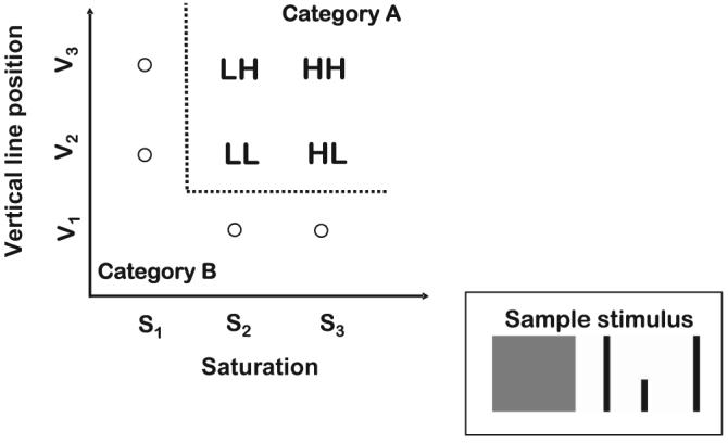
Schematic illustration of the conjunctive-rule category structure tested in Experiments 1 and 2. L = low-intensity target; H = high-intensity target.

The category structure is illustrated in Figure 5. Membership in Category A is defined by a conjunctive rule. A stimulus is a member of the category if it has a saturation value greater than or equal to S2 and has a vertical line value greater than or equal to V2. The remaining stimuli are members of Category B.

The four members of Category A have the same structure as illustrated previously for the double-target stimuli of the detection paradigm (cf. Figures 1 and 5). Values of S3 and V3 are easier to discriminate from the contrast category than are values of S2 and V2. Thus, values of S3 and V3 correspond to the high-salience values in the factorial manipulation, whereas values of S2 and V2 correspond to the low-salience values. The four stimuli S2-V2, S2-V3, S3-V2, and S3-V3 correspond to the LL, LH, HL, and HH stimuli, respectively.

Note that in the example in our introduction, the visual detection task had the form of an or paradigm. The task was to detect whether a target was present in either the left visual field or in the right visual field. By contrast, with respect to the category of LL, LH, HL, and HH stimuli, the present classification task involves use of an and paradigm. A stimulus is a member of Category A only if it has a sufficiently large magnitude on the saturation dimension and a sufficiently large magnitude on the vertical line dimension.⁵ Given the nature of the and paradigm, only a subset of the processing architectures discussed previously are plausible candidates for a classification strategy. In particular, it would be implausible to see evidence of any form of self-terminating processing in the present case. For example, classifying an item as having a saturation value of greater than or equal to S2 does not provide sufficient information to determine that it is a member of Category A. The item must also have a vertical line value of greater than or equal to V2. Both dimensions must be processed to allow appropriate Category A membership decisions. Thus, in the present case, the candidate processing architectures correspond to serial-exhaustive, parallel-exhaustive, or coactive processing of the dimensions. Because of the highly separable nature of the stimulus dimensions, however, our key hypothesis was that we would not see evidence of coactive processing in the present experiment.

Method

Subjects

The subjects were 7 graduate and undergraduate students associated with Indiana University. All subjects were under 40 years of age and had normal or corrected-to-normal vision. The subjects were paid $8 per session plus up to a $3 bonus per session depending on performance.

Stimuli

In the nonoverlapping condition, each stimulus consisted of two spatially separated rectangular regions. The left rectangle had a red hue that varied in its saturation, and the right rectangular region had an interior vertical line that varied in its left–right positioning. In the overlapping condition, the hue and the line were presented in a single rectangle.

As illustrated in Figure 5, there were eight stimuli composed of the factorial combination of three values of saturation and three values of vertical line position (with Stimulus S1-V1 deleted from the set). The saturation values were derived from the Munsell color system, and we generated them on the computer by using the Munsell color conversion program (WallkillColor, Version 6.5.1; Van Aken, 2006). According to the Munsell system, the colors were of a constant red hue (5R) and of a constant lightness (Value 5) but had saturation (chromas) equal to 10, 8, and 6, respectively. The resulting red–green–blue (RGB) values for the colors are reported in Table 2. Likewise, the distances of the vertical line relative to the leftmost side of the right rectangle are also presented in Table 2. The size of each rectangle was 133 × 122 pixels. In the nonoverlapping condition, the rectangles were separated by 45 pixels, and each pair of rectangles subtended a horizontal visual angle of about 6.4° and a vertical visual angle of about 2.3°. In the overlapping condition, the single rectangle subtended a horizontal visual angle of about 2.5° and a vertical angle of about 2.3°. We used a Pentium PC to run the study on a CRC monitor, with display resolution 1024 × 768 pixels.

Table 2.

Experiment 1: Red, Green, and Blue Values and Vertical-Line Distance (Measured in Pixels) for Each of the Stimuli in the Separable-Dimension Experiment

Stimulus	Red	Green	Blue	Distance
S1-V2	194	90	87	40
S1-V3	194	90	87	50
S2-V1	181	98	94	30
S2-V2	181	98	94	40
S2-V3	181	98	94	50
S3-V1	168	105	101	30
S3-V2	168	105	101	40
S3-V3	168	105	101	50

Note. S = saturation; V = vertical-line position.

Procedure

The stimuli were divided into two categories, A and B, as illustrated in Figure 5. On each trial, a single stimulus was presented, the subject was instructed to classify it into Category A or B as rapidly as possible without making errors, and corrective feedback was then provided.

At the start of the experiment, subjects were shown a picture of the complete stimulus set (in the form illustrated in Figure 5, except with the actual stimuli displayed). The subjects were provided with explicit instructions concerning the nature of the category structure. The instructions pointed out that the members of Category B each possessed one of two extreme values: They were either the most saturated with red or contained a vertical line that was positioned farthest to the left. By contrast, Category A consisted of items that had less extreme values on both dimensions. The reason for illustrating the full stimulus set and for providing explicit instructions about the category structure was to speed classification learning and to make the data collection process more efficient.

The experiment was conducted over five sessions, one session per day, with each session lasting approximately 45 min. In each session, subjects received 24 practice trials and then were presented with 744 experimental trials. Trials were grouped into six blocks, with rest breaks in between each block. Each stimulus was presented the same number of times within each session. Thus, for each subject, each stimulus was presented 93 times per session and 465 times over the course of the experiment. The order of presentation of the stimuli was randomized anew for each subject and session.

Subjects made their responses by pressing the right (Category A) and left (Category B) buttons on a computer mouse. The subjects were instructed to rest their index fingers on the mouse buttons throughout the testing session. RTs were recorded from the onset of a stimulus display up to the time of a response. Each trial consisted of the presentation of a central fixation point (crosshair) and a high-pitched warning tone for 1,770 ms, with the onset of the tone coming 1,070 ms after the fixation point (i.e., the duration of the tone was 700 ms). The stimulus was then presented on the screen and remained visible until the subject's response was recorded. In the case of an error, corrective feedback was provided for 2 s. The intertrial interval was 1,870 ms.

Results

Session 1 was considered practice, and these data were not included in the analyses. In addition, conditionalized on each individual subject and stimulus condition (HH, LH, HL, and LL), we removed from the analysis RTs greater than three standard deviations above the mean and also RTs of less than 100 ms. This procedure led to dropping less than 1.4% of the trials from analysis.

We examined the mean RTs for the individual subjects as a function of sessions of testing. Although there was a general speeding of RTs (see Figure 6), the basic pattern for the HH, HL, LH, and LL stimuli remained constant across sessions. Therefore, we combine the data across sessions in illustrating the results.

Figure 6.

Experiment 1: Mean response times (RTs) for the individual subjects (Sub) plotted as a function of sessions of testing.

The mean RTs for the HH, HL, LH, and LL stimuli are shown for the individual subjects in the leftmost column of Figure 7, and the error rates are reported in Table 3. It is clear from inspection that, for all 7 subjects, the manipulations of saturation and vertical-line position had the expected effects on the overall pattern of mean RTs, in the sense that the high-salience values led to faster RTs than did the low-salience values. The pattern of errors mirrored the RT results. That is, higher error rates were associated with slower mean RTs.

Figure 7.

(opposite) Experiment 1: The systems factorial technology (SFT) results for the separable-dimension stimuli. Shown are mean response times (RTs; left), survivor functions (middle), and survivor interaction contrast (SIC) function (right). L = low-intensity target; H = high-intensity target; T = time of processing; t = time units.

Table 3.

Experiment 1 (Separable Dimensions): Proportion of Classification Errors Observed for Each Subject in Each Factorial Condition

	Condition
Subject	HH	HL	LH	LL
Nonoverlapping spatial positions
1	.02	.06	.05	.12
2	.00	.01	.01	.04
3	.00	.04	.03	.07
4	.01	.09	.08	.39
5	.03	.11	.11	.27
Overlapping spatial positions
6	.00	.04	.01	.06
7	.00	.05	.03	.10

Note. H = high-intensity target; L = low-intensity target.

The critical question concerns the results for the MIC. Inspection of Figure 7 suggests an additive pattern for Subjects 1, 2, 3, 5, and 7 and an underadditive pattern for Subject 4 and perhaps Subject 6. This impression is confirmed by statistical test. Specifically, for each individual subject, we conducted three-way analyses of variance (ANOVAs) on the RT data using as factors session (2–5), level of saturation (H or L), and level of vertical-line position (H or L). The results of the ANOVAs are summarized in Table 4. The main effects of saturation and line position (not reported in the table) were highly significant for all subjects. The interaction between saturation and line position did not approach statistical significance for Subjects 1, 2, 3, 5, or 7, supporting the conclusion of an additive pattern of mean RTs (MIC = 0) for these subjects. This result suggests that these subjects engaged in serial processing of the dimensions (see Table 1). By contrast, the interaction between saturation and line position was statistically significant for Subject 4 and was marginally significant for Subject 6. The underadditive pattern of mean RTs suggests that Subject 4 and perhaps Subject 6 engaged in parallel-exhaustive processing to classify the Category A stimuli (see Table 1). The most critical result is that there is no evidence of an overadditive MIC for any of the subjects, indicating the absence of coactive processing of the dimensions. Because Subjects 4 and 5 had high error rates on the LL stimulus (see Table 3), we need to express caution about the processing architecture that we infer for them (see Appendix A). However, the remaining 5 subjects all had relatively low error rates for all of the stimuli, and these subjects too show no evidence of coactive processing.

Table 4.

Experiment 1 (Separable Dimension Stimuli): Individual Subject ANOVA Results

Subject and factor	df	F	p	ηp2
Nonoverlapping spatial positions
Subject 1
Session	3	9.789	.000	.022
Saturation × Line Position	1	.962	.327	.001
Saturation × Line Position × Session	3	.614	.606	.001
Error	1317
Subject 2
Session	3	85.491	.000	.156
Saturation × Line Position	1	.102	.749	.000
Saturation × Line Position × Session	3	.766	.513	.002
Error	1388
Subject 3
Session	3	210.501	.000	.318
Saturation × Line Position	1	.738	.391	.001
Saturation × Line Position × Session	3	.522	.667	.001
Error	1355
Subject 4
Session	3	143.022	.000	.264
Saturation × Line Position	1	6.477	.011	.005
Saturation × Line Position × Session	3	3.707	.011	.009
Error	1197
Subject 5
Session	3	107.128	.000	.208
Saturation × Line Position	1	.038	.846	.000
Saturation × Line Position × Session	3	1.565	.196	.004
Error	1222
Overlapping spatial positions
Subject 6
Session	3	5.287	.001	.012
Saturation × Line Position	1	2.989	.084	.002
Saturation × Line Position × Session	3	1.436	.230	.003
Error	1361
Subject 7
Session	3	7.916	.000	.017
Saturation × Line Position	1	.191	.662	.000
Saturation × Line Position × Session	3	.572	.633	.001
Error	1338

Note. The error row defines the degrees of freedom for the F test error term, for that subject. Each F test value has two degrees of freedom: one from its corresponding row, and the other from the error row.

The main effect of sessions was statistically significant for all subjects, reflecting a generalized speeding of performance (for most of the subjects) as a function of practice in the task (see Figure 6). However, with the exception of Subject 4, there were no interactions of session with the other factors, reflecting the fact that the overall pattern of RTs was fairly stable throughout testing. Closer inspection of Subject 4's data suggested that a pattern of RT underadditivity during the early sessions gave way to a pattern of additivity during the later ones.

The next step in the analysis was to compute the survivor functions associated with each of the stimuli as well as the SIC function. We computed these functions by dividing the full distribution of RT data into 10-ms bins and computing the probability that RT exceeded the upper limit of each bin value. The survivor functions for the individual HH, LH, HL, and LL stimuli are shown for each individual subject in the middle column of Figure 7, and the computed SIC functions are shown in the right column. A requirement for meaningful application of the SIC test is that the survivor functions be ordered in a nonoverlapping manner such that, for all time values t, S_LL (t) > S_LH (t), S_HL (t) > S_HH (t). For details, see Townsend and Nozawa (1995). As can be seen in Figure 7, this requirement is satisfied for all subjects.

The SIC functions, shown in the far right column of Figure 7, have the signature of serial-exhaustive processing for Subjects 1, 2, 3, 5, and 7 (cf. Figure 4B). At early time values, the SIC functions are negative, and they switch to positive for larger time values. Furthermore, the areas of the negative and positive regions are approximately equal to one another, as already indicated by our previous statistical tests showing that the MIC values did not differ significantly from zero.⁶ For Subjects 4 and 6, the SIC functions have the signature of parallel-exhaustive processing (cf. Figure 4D). In particular, the SIC functions are negative essentially throughout, consistent with the previous statistical tests showing a negative (underadditive) value of the MIC for those subjects.

To address the possibility that the forms of the SIC functions were contaminated by the general speeding that was observed across sessions, we conducted additional analyses in which the RT distributions were detrended. Specifically, for each individual subject, we subtracted the mean RT for a given session from all individual RTs obtained in that session. We then recomputed the survivor and SIC functions from these detrended data. The computed functions were essentially identical in form to those that we have already displayed in Figure 7.

In summary, taken together, the MIC and SIC results show evidence of use of an exhaustive stopping rule for all subjects, which appears to be a necessary processing strategy for classifying the members of the conjunctive-rule (and) structure associated with Category A. Furthermore, 5 of the subjects showed clear evidence of serial processing of the dimensions, whereas 2 subjects showed some evidence of parallel processing. Most important, the MIC and SIC results provide no evidence of coactive processing of the dimensions, as we would expect given the highly separable nature of the present stimulus dimensions. We turn now to an analogous experiment involving the use of integral-dimension stimuli, where we expect a dramatic turnaround. In particular, in conditions involving the classification of integral-dimension stimuli, the SFT methodology should instead provide clear-cut evidence of coactive processing of the dimensions.

Experiment 2: Classification of Integral-Dimension Stimuli

In Experiment 2, we used the same type of category structure and task as in Experiment 1. The only difference is that the stimuli now varied along integral dimensions (Munsell colors varying in brightness and saturation) instead of separable dimensions. There were three equally spaced saturation values (S1, S2, and S3) combined factorially with three equally spaced brightness values (B1, B2, and B3) to yield a stimulus structure directly analogous to the separable-dimension structure illustrated previously in Figure 5. Members of Category A were defined by the same type of conjunctive rule as used in the previous experiment, thereby creating the LL, LH, HL, and HH stimulus types.

One limitation in the testing of integral-dimension stimuli is that it is impossible to produce a configuration with a perfectly gridlike structure in an individual's psychological space. That is, given the nature of integral-dimension stimuli, a person's perception, say, of level of brightness may be influenced by level of saturation and vice versa (Ashby & Townsend, 1986). We conducted independent similarity-scaling studies for the colors and used the similarity data to derive multidimensional scaling (MDS) solutions. As reported in Appendix B, the resulting MDS solutions well approximated the intended 3 × 3 factorial structure of the stimulus sets, but of course some distortions were present. In an attempt to address the role that such distortions may have on the computed MIC values and SIC functions, we instantiated the abstract experimental design with two different sets of Munsell colors. To the extent that the same patterns of results are observed across sets, we gain confidence that the results are due to the integral nature of the perceptual dimensions and not to artifacts involving specific individual stimuli or sets.

Method

Subjects

The subjects were 8 graduate and undergraduate students associated with Indiana University. All subjects were under 40 years of age and had normal or corrected-to-normal vision. The subjects were paid $8 per session plus up to a $3 bonus per session depending on performance.

Stimuli

According to the Munsell system, for both sets of stimuli, the colors were of a constant red hue (5R). Set 1 was constructed by combining orthogonally Saturation (chroma) Values 10, 8, and 6 with Brightness Values 4, 5, and 6 (but with the combination Saturation-10/Brightness-4 deleted from the set). Set 2 was the same, except we used Brightness Values 5, 6, and 7 instead. (All nine stimuli were presented in the conditions involving Set 2.) According to the Munsell system, all adjacent stimuli were equally spaced along the brightness and saturation dimensions. The resulting stimulus configurations and category structures therefore had the same schematic structure as illustrated previously in Figure 5.

We generated the stimuli by using the Munsell color conversion program (WallkillColor, Version 6.5.1) and conducted MDS studies to verify that the generated colors provided a good approximation of the intended 3 × 3 factorial structure (see Appendix B). The RGB values for each stimulus are presented in Table 5. The colors were presented as rectangular shapes, 133 × 122 pixels in size, centered on the computer screen with a white background. Each stimulus subtended a horizontal visual angle of about 2.5° and a vertical visual angle of about 2.3°. The same apparatus was used as in Experiment 1.

Table 5.

Experiment 2: Red, Green, and Blue Values for Each Stimulus in the Integral-Dimension Experiment

Stimulus	Red	Green	Blue
Set 1
S1-B2	194	90	87
S1-B3	154	72	71
S2-B1	141	80	77
S2-B2	181	98	94
S2-B3	208	125	119
S3-B1	222	117	112
S3-B2	168	105	101
S3-B3	195	131	126
Set 2
S1-B1	194	90	87
S1-B2	222	117	112
S1-B3	253	143	136
S2-B1	181	98	94
S2-B2	208	125	119
S2-B3	238	151	144
S3-B1	168	105	101
S3-B2	195	131	126
S3-B3	223	157	151

Note. S = saturation; B = brightness.

Procedure

The procedure was the same as in Experiment 1.

Results

We analyzed only the data from Sessions 2–5. We again deleted from analysis all trials in which the RT was greater than three standard deviations above the mean for each given subject–stimulus combination. We also deleted trials in which the RT was less than 100 ms. This procedure led to deleting less than 1.8% of the trials.

Visual inspection of the data indicated that the pattern of mean RTs was the same across sessions. Therefore, in illustrating the summary results, we present mean RTs that are combined across the sessions.

The mean RTs for the HH, HL, LH, and LL stimuli are shown for the individual subjects in the leftmost column of Figure 8, and the error rates are reported in Table 6. As was the case for the separable-dimension stimuli, the high-salience dimension values always led to faster RTs than did the low-salience ones, and the error rates mirrored the RTs.

Figure 8.

(opposite). Experiment 2: The systems factorial technology (SFT) results for the integral-dimension stimuli. Shown are mean response times (RTs; left), survivor functions (middle), and survivor interaction contrast (SIC) function (right). L = low-intensity target; H = high-intensity target; T = time of processing; t = time units.

Table 6.

Experiment 2 (Integral Dimensions): Proportion of Classification Errors Observed for Each Subject in Each Factorial Condition

	Condition
Subject	HH	HL	LH	LL
Set 1
1	.00	.09	.03	.31
2	.00	.02	.00	.04
3	.00	.01	.00	.11
4	.01	.06	.04	.16
5	.00	.01	.01	.17
Set 2
6	.01	.03	.08	.39
7	.00	.01	.01	.09
8	.00	.02	.03	.23

Note. H = high-intensity target; L = low-intensity target.

In dramatic contrast to the results from Experiment 1, however, inspection of Figure 8 reveals a strongly overadditive pattern of mean RTs for almost all subjects. To confirm this observation, we conducted three-way ANOVAs on the individual subjects' RT data, using session, saturation level, and brightness level as factors. The results are reported in Table 7. The most important result is that, for all subjects except for Subject 1 in the Set 1 condition, there was a statistically significant interaction between saturation level and brightness level. That is, the MIC value was significantly greater than zero. Thus, the overadditive pattern of mean RTs observed in Figure 8 is statistically significant at the level of individual subjects. This overadditive pattern in the mean RTs provides a signature that processing is either parallel self-terminating or coactive (see Table 1). Because the logical structure of the conjunctive-rule classification eliminates the possibility of a self-terminating decision strategy, however, we expect the subsequent SIC tests to point clearly to a coactive processing architecture.

Table 7.

Experiment 2 (Integral Dimension Stimuli): ANOVA Results for the Individual Subjects

Subject and factor	df	F	p	ηp2
Set 1
Subject 1
Session	3	9.082	.000	.021
Saturation × Brightness	1	.586	.444	.000
Saturation × Brightness × Session	3	5.046	.002	.012
Error	1252
Subject 2
Session	3	53.063	.000	.104
Saturation × Brightness	1	17.825	.000	.013
Saturation × Brightness × Session	3	2.312	.074	.005
Error	1377
Subject 3
Session	3	165.519	.000	.268
Saturation × Brightness	1	13.798	.000	.010
Saturation × Brightness × Session	3	1.836	.139	.004
Error	1358
Subject 4
Session	3	26.932	.000	.058
Saturation × Brightness	1	51.606	.000	.038
Saturation × Brightness × Session	3	3.150	.024	.007
Error	1307
Subject 5
Session	3	15.022	.000	.033
Saturation × Brightness	1	23.169	.000	.017
Saturation × Brightness × Session	3	.520	.669	.001
Error	1340
Set 2
Subject 6
Session	3	13.278	.000	.031
Saturation × Brightness	1	7.553	.006	.006
Saturation × Brightness × Session	3	1.668	.172	.004
Error	1227
Subject 7
Session	3	35.791	.000	.073
Saturation × Brightness	1	10.684	.001	.008
Saturation × Brightness × Session	3	.182	.909	.000
Error	1367
Subject 8
Session	3	18.305	.000	.040
Saturation × Brightness	1	13.750	.000	.010
Saturation × Brightness × Session	3	2.161	.091	.005
Error	1304

Note. The error row defines the degrees of freedom for the F test error term, for that subject. Each F test value has two degrees of freedom: one from its corresponding row, and the other from the error row.

The mean RTs, averaged across all stimuli, are shown as a function of sessions of testing in Figure 9. As can be seen in the figure, for most subjects there was again a generalized speed-up as a function of sessions. This main effect of sessions was statistically significant for all subjects (see Table 7). There was also a statistically significant interaction among sessions, saturation, and brightness for many of the individual subjects (see Table 7). Visual inspection of the individual-session data suggests, however, that the basic form of the overadditive MIC was reasonably consistent throughout, with only its quantitative magnitude varying across the sessions of testing. We did not observe any systematic increase or decrease in the magnitude of the overadditivity as a function of sessions.

Figure 9.

Experiment 2: Mean response times (RTs) for the individual subjects (Sub) plotted as a function of sessions of testing.

The survivor functions for the individual HH, LH, HL, and LL stimuli, as well as the SIC functions, are shown in Figure 8. With the exception of Subject 1 in the Set 1 condition, the SIC functions possess an obvious signature of a coactive processing architecture. In all of these cases, there is an initial time period in which the SIC functions are negative, followed by a longer time period in which the SIC functions are positive. The area under the positive regions exceeds the area in the negative regions, which corresponds to the overadditive pattern in the mean RTs seen earlier. In additional analyses in which we detrended the individual RTs to remove any overall effect of sessions, the form of the computed SIC functions remained the same.

Interestingly, the single subject who failed to show an overadditive MIC (Subject 1) had a high error rate (.31) on the LL stimulus, whereas almost all other subjects had low to moderate error rates. As indicated by our simulations in Appendix A, a high error rate can cause the overadditive signature of coactive processing to disappear, which provides a potential explanation for Subject 1's results.

In summary, the results from the present experiment provide a dramatic turnaround compared with the results from Experiment 1. As expected, for the present case involving integral-dimension stimuli, the MIC and SIC results provide compelling evidence of coactive processing of the dimensions.

General Discussion

Summary

In summary, the purpose of this work was to provide a validation test of the SFT applied in the domain of multidimensional classification. The SFT has been developed to diagnose the nature of the information-processing architectures that underlie multidimensional perception and cognition. Most previous applications of the SFT have taken place in the domains of detection and visual and short-term memory search. In the present research, we extended the applications to classification decision making.

Specifically, in the present tests, subjects classified objects into a conjunctive-rule category structure. Furthermore, in one experiment, the stimuli varied along highly separable dimensions, whereas in a second experiment the stimuli varied along integral dimensions. On the basis of a long history of converging evidence, we reasoned that coactive processing takes place when observers classify integral-dimension stimuli, whereas there should be no coactive processing in the classification of highly separable-dimension stimuli. The present tests yielded strong positive evidence in accord with this line of reasoning. In the experiment involving highly separable-dimension stimuli, the SFT tests involving the computation of the MIC and SIC indicated that coactive processing of dimensions did not occur. By contrast, clear evidence for the presence of coactive processing was obtained in the experiment involving integral-dimension stimuli. The results thereby provide a striking validation of the SFT as an instrument for diagnosing information-processing architectures in the domain of multidimensional perceptual classification.

Relation to Miller's (1982) Inequality

One of the major past approaches to testing for coactivation in the processing of multidimensional stimuli involves the application of Miller's (1982) inequality. Although this approach provides an extremely useful diagnostic, the current SFT methodology offers some significant advances. In an application of Miller's inequality, the complete set of stimuli has a structure analogous to the LL, LH, HL, and HH stimuli that compose the target category of the double factorial paradigm. The subject's task is to determine whether either dimension of a presented stimulus has a high-salience value. (In most previous applications of the test, L and H have corresponded to absence versus presence of a stimulus component, but other applications have involved different levels of an always-present component). Thus, with respect to the target category of LH, HL, and HH stimuli, this paradigm involves use of an or task. The question addressed by tests of Miller's inequality is whether the facilitation observed for the redundant-signals HH stimulus compared with the single-signals LH and HL stimuli goes beyond the pure statistical facilitation that is predicted by an unlimited-capacity parallel self-terminating model. As noted by Miller, the parallel self-terminating model predicts that for all time values t,

$$p_{\mathrm{HH}}(\mathrm{RT}<t)\le p_{\mathrm{LH}}(\mathrm{RT}<t)+p_{\mathrm{HL}}(\mathrm{RT}<t),$$

where p_ij(RT < t) is the probability that the RT for determining that stimulus ij has Level H on one of its dimensions is less than or equal to t. Note that for large values of t, the inequality is satisfied in trivial fashion, because as t → ∞, p_ij(RT < t) → 1. However, for small values of t, it is logically possible for the inequality to be violated (i.e., that the redundant-signals cumulative probability on the left exceeds the sum of the single-signals cumulative probabilities on the right). Such a violation of Miller's inequality is often interpreted as providing evidence in favor of coactive processing of the dimensions.

Although a violation of Miller's (1982) inequality does rule out the parallel self-terminating model (assuming that various technical assumptions are satisfied), other processing architectures can produce such a violation without any coactivation occurring. For example, Townsend and Nozawa (1997) pointed out that in cases in which high-intensity values are processed much faster than are low-intensity values, serial exhaustive models predict violations of the inequality. To see this intuitively, note that if high-intensity values are processed very rapidly, then serial exhaustive models predict that p_HH(RT < t) can be very large even for small values of t. And if low-intensity values are processed very slowly, then p_LH(RT < t) and p_HL(RT < t) can both be very small at these same values of t. This combination of events would lead to a violation of the inequality. Furthermore, serial-exhaustive processing is a logical possibility for the redundant-signals (or) paradigm (even though intuition suggests that a self-terminating stopping rule might govern performance; cf. Sternberg, 1969). The significant advance provided by the SFT methodology is that it provides a simultaneous diagnosis of questions involving architecture, stopping rule, and capacity, thereby allowing stronger conclusions as to whether coactive processing of dimensions has actually occurred.

Converging Operations

The focus of this research was to provide validation tests of the SFT methodology in the domain of multidimensional perceptual classification. Viewed from another perspective, however, this research adds to the list of converging operations that have been used to distinguish between integral dimensions and separable dimensions. In Garner's (1974) speeded classification tasks, for example, it is well documented that, relative to a baseline condition, integral dimensions yield interference in the filtering task and facilitation in the correlated task, whereas separable dimensions do not yield interference or facilitation. Similarity-scaling research suggests an approximate Euclidean metric underlying distance relations among integral-dimension stimuli but a more nearly city-block metric underlying distance relations among separable-dimension stimuli (Garner, 1974; Shepard, 1964). Work in multidimensional categorization suggests that, in the case of highly separable dimensions, observers selectively attend to component dimensions both in learning and in generalizing to novel transfer stimuli (Kruschke, 1993; Nosofsky, 1989; Shepard, Hovland, & Jenkins, 1961). By contrast, this type of selective attention process is far less efficient in the case of integral-dimension stimuli (McKinley & Nosofsky, 1996; Nosofsky & Palmeri, 1996; Shepard & Chang, 1963).

Now added to this list of converging operations are the present SFT results that test for the presence of coactive processing. Integral-dimension stimuli give rise to an overadditive pattern of mean RTs in the double-factorial paradigm. Furthermore, the SIC function shows a clear negative blip at early time periods, followed by more extensive positivity at later time periods. By contrast, separable-dimension stimuli give rise to an additive or underadditive pattern of mean RTs in the double-factorial paradigm. In addition, the SIC function has a form that is clearly distinct from the one yielded by integral-dimension stimuli.

Future Research Directions

An important topic for future research is to consider other processing architectures that might account for the pattern of results observed in our experiments. One possibility involves a very general class of models in which separate dimensions facilitate one another through parallel channel interactions. In this case, information might be shared, or activation on one channel might cross over and help activate a separate channel (Mordkoff & Yantis, 1991; Townsend & Wenger, 2004b). Unlike true coactivation models, this kind of processing still involves separate detection criteria operating in each channel. Nevertheless, we know that an extreme special case of interactive parallel models is the class of coactivation models,⁷ so interactive parallel models must be able to produce coactivation predictions. Nonetheless, at present, we understand very little about their generic predictions or if, say, the coactive type of prediction comes naturally to the overall class.

Yet another target for future research is to consider the predictions from modern process-based models of multidimensional classification (e.g., Ashby, 2000; Lamberts, 2000; Nosofsky & Palmeri, 1997b; Ratcliff & Rouder, 1998; Thomas, 2006). For example, according to Nosofsky and Palmeri's (1997b) exemplar-based random-walk model, people classify objects by retrieving individual category exemplars from memory. The retrieved exemplars drive a random-walk process that leads to classification decisions. Preliminary simulation work suggests that, for the present double-factorial classification paradigm, the exemplar-based random-walk model yields MIC and SIC signatures of coactive processing across a wide range of its parameter space. (For closely related investigations of process-model signatures in cases in which other experimental variables are manipulated, see Thomas, 2006.) It is an open question whether such models can account jointly for the patterns of RT results seen in the present experiments involving separable-dimension and integral-dimension stimuli.

Appendix A

Simulations of Serial, Parallel, and Coactive Process Models

In this appendix, we report simulations of serial, parallel, and coactive architectures in which the component processes are represented in terms of random-walk models that give rise to errors. The simulations are conducted with respect to the conjunctive-rule (and) structure depicted in Figure 5. Thus, we consider the case of only an exhaustive stopping rule and derive simulated predictions for the LL, LH, HL, and HH stimuli (where L refers to low intensity and H refers to high intensity). From these simulated predictions, we then compute the predicted mean interaction contrast (MIC) and survivor interaction contrast (SIC) signatures for the different processing architectures.

According to the serial and parallel models, separate decisions are made along each of dimensions x and y, and these decisions are then combined in making the overall response. The decision along each individual dimension is governed by a separate random-walk process (for a detailed description, see Nosofsky & Stanton, 2005, pp. 609–611, 625). In brief, for each dimension, there is a random-walk counter with initial value zero. The observer establishes criteria, +A and −B, representing the amount of evidence needed for making a Category A or Category B decision. Given presentation of stimulus i, on each step of the random walk there is a probability p_i that the counter is incremented by unit value in the direction of Criterion +A, whereas with probability 1− p_i the counter is decremented by unit value in the direction of Criterion −B. (We describe below how the stimulus-specific step probabilities p_i are computed.) If the counter reaches Criterion +A, then a Category A decision is made on that dimension, whereas if the counter reaches Criterion −B, then a Category B decision is made. The time to make a decision for each dimension is determined by the number of steps required to complete each random walk. Note that for the present conjunctive-rule and structure, a correct Category A response is made only if the decisions on both individual dimensions point to A. If the decision on either individual dimension points to Category B, then an incorrect Category B response is made. The random-walk decision processes along each dimension are assumed to operate independently.

For the serial-exhaustive model, the time to make a correct Category A response is given by the sum of the two individual random-walk times on each trial. For the parallel-exhaustive model, the time to make a correct Category A response is given by the maximum of the two individual random-walk times on each trial. The simulations also included a log-normally distributed base time that was added to the decision time described above. The distribution of base times was identical for the LL, LH, HL, and HH stimuli.

The stimulus-specific step probabilities (p_i) for each random walk are computed as follows. Along each individual dimension, the H, L, and nontarget (0) stimuli are assumed to be arrayed in the form shown in Figure A1. In accord with standard signal-detection theory, we assume that there is a normal distribution of perceptual effects associated with each stimulus. As shown in the figure, the stimulus levels are assumed to be equally spaced with means μ_H = 3, μ_L = 2, and μ₀ = 1. Each stimulus distribution is assumed to have a common perceptual variance σ²_p. The observer establishes a decision boundary between the L and the 0 stimuli to partition the space into decision regions. On each step of the random walk, a perceptual effect is sampled from the relevant stimulus distribution. If the perceptual effect falls in Region A, then the random-walk counter is incremented toward Criterion +A, whereas if the perceptual effect falls in Region B, then the counter is decremented toward Criterion −B. Thus, on each step, the probability p_i that the random walk is incremented in the direction of Criterion +A is given by the proportion of the stimulus i distribution that falls in Region A. Note that this step probability will be higher for H stimuli than for L stimuli, so responses for stimuli with high-salience dimension values will tend to be faster and less error prone than for those with low-salience values.

Figure A1.

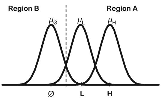
Schematic illustration of the perceptual sampling process that determines the step probabilities in the random-walk versions of the simulated serial, parallel, and coactive models. L = low-intensity target; H = high-intensity target.

To simulate the coactive model, we assumed that the perceptual sampling processes along each dimension operated in tandem and contributed counts to a common random walk. On each step, if the sampled perceptual effects on both dimensions x and y fell in their respective Region As, then the common random-walk counter was incremented by unit value in the direction of Criterion +A. If both sampled perceptual effects fell in their respective Region Bs, then the counter was decremented by unit value in the direction of Criterion −B. Finally, we investigated two different versions of the coactive model for the case in which the sampled perceptual effects provided conflicting information. In Version 1, if the sampled perceptual effect for one dimension fell in Region A but the sampled perceptual effect for the second dimension fell in Region B, then the random-walk counter was not incremented or decremented on that step. In Version 2, we assumed that the random-walk counter was decremented by unit value toward −B if either perceptual effect fell in Region B. In all other respects, the random-walk process for the coactive model was the same as for the serial and parallel models described previously.

The results from representative versions of these simulations are reported in Tables A1-A4 for the serial, parallel, and coactive models. Each result is based on 30,000 simulations for each individual LL, LH, HL, and HH stimulus. In these representative simulations, for all of the random-walk processes, we set |+A| = |−B| = 5. Also, we set the decision boundary for each perceptual sampling process midway between the means of the L and nontarget stimuli shown in Figure A1. To simulate the base time from a log-normal distribution, we chose a random value from a normal distribution with mean μ = 6 and standard deviation σ = .3, and this random value was exponentiated. Also, the number of steps in each random walk was multiplied by an arbitrary scaling constant k = 10. We chose these parameter values to place the simulated response times from the models in roughly the same range as observed for the subjects, but the fundamental qualitative predictions from the models do not depend on these choices. Finally, to study the behavior of the models in the face of increasing error rates, we varied the magnitude of the perceptual variance parameter σ²_p. As the magnitude of the perceptual variance increases, there is a higher probability that the random walks take steps in the wrong direction, so error rates increase. Simulated response times were computed conditional on correct responses only, as was the case in our reports of the observed data.

Table A1.

Serial Model Simulations

	Stimulus type
	HH		HL		LH		LL
σp	RT	p(E)	RT	p(E)	RT	p(E)	RT	p(E)	MIC
.50	522	.00	546	.00	545	.00	568	.00	−.6
.75	527	.00	575	.00	574	.00	622	.01	.7
1.00	538	.00	605	.02	605	.02	675	.04	2.2
1.25	552	.00	635	.04	637	.04	720	.08	.0
1.50	568	.00	662	.07	662	.06	754	.13	−1.1
1.75	585	.00	685	.09	685	.09	785	.17	−.5
2.00	604	.00	708	.12	708	.12	808	.23	−1.8
2.25	622	.01	725	.15	724	.15	828	.27	1.6
2.50	640	.02	741	.17	742	.17	841	.31	−1.7
2.75	657	.03	755	.20	754	.20	852	.34	.1
3.00	674	.03	769	.22	766	.22	862	.37	1.1
3.25	691	.05	781	.24	778	.24	870	.40	1.1

Note. H = high-intensity target; L = low-intensity target; RT = mean response time; p(E) = proportion of errors; MIC = mean interaction contrast.

Table A4.

Coactive Model Simulations, Version 2

	Stimulus type
	HH		HL		LH		LL
σp	RT	p(E)	RT	p(E)	RT	p(E)	RT	p(E)	MIC
.50	472	.00	495	.00	496	.00	539	.01	20.0
.55	473	.00	502	.00	501	.00	561	.03	30.0
.60	473	.00	507	.00	507	.00	584	.06	43.4
.65	475	.00	514	.00	515	.00	609	.10	55.2
.70	474	.00	521	.00	520	.00	629	.16	62.3
.75	478	.00	529	.01	529	.01	646	.23	65.7
.80	479	.00	538	.01	539	.01	661	.31	62.7
.85	481	.00	546	.02	547	.02	669	.40	57.3
.90	483	.00	556	.02	557	.02	672	.48	42.7

Note. H = high-intensity target; L = low-intensity target; RT = mean response time; p(E) = proportion of errors; MIC = mean interaction contrast.

Figure A2.

Simulated survivor interaction contrast functions for serial, parallel, and coactive models (30.000 simulations per condition) for cases in which the error rate on the LL stimulus is approximately .20. SIC = survivor interaction contrast; t = time units; L = low-intensity target; H = high-intensity target; RT = response time.

Inspection of Table A1 reveals that, for the serial exhaustive model, the simulated MICs hover around zero (additivity) throughout, even as error rates get very high. Table A2 reveals that, for the parallel exhaustive model, the simulated MICs are decidedly negative (under-additive) throughout, even as error rates get very high. For Version 1 of the coactive model (see Table A3), the simulated MICs are clearly positive (overadditive) for low and moderate error rates. However, as error rates get very high (roughly .30 for the LL stimulus), the overadditivity disappears and the MIC instead falls back to near zero. Finally, for Version 2 of the coactive model (see Table A4), the MICs are clearly positive even for very high error rates.

Table A2.

Parallel Model Simulations

	Stimulus type
	HH		HL		LH		LL
σp	RT	p(E)	RT	p(E)	RT	p(E)	RT	p(E)	MIC
.50	473	.00	495	.00	495	.00	509	.00	−8.3
.75	478	.00	522	.01	523	.01	550	.01	−18.1
1.00	486	.00	550	.02	550	.02	587	.04	−27.6
1.25	497	.00	574	.04	574	.04	621	.08	−31.0
1.50	510	.00	594	.07	594	.06	647	.13	−30.7
1.75	523	.00	610	.09	610	.09	670	.17	−27.1
2.00	535	.00	627	.12	625	.12	688	.22	−29.1
2.25	549	.01	639	.15	637	.15	699	.27	−27.3
2.50	563	.02	648	.18	647	.18	712	.30	−20.8
2.75	574	.02	657	.20	658	.20	720	.34	−20.8
3.00	588	.03	668	.22	666	.22	727	.37	−18.4
3.25	601	.05	676	.25	674	.25	733	.40	−15.4

Note. H = high-intensity target; L = low-intensity target; RT = mean response time; p(E) = proportion of errors; MIC = mean interaction contrast.

Table A3.

Coactive Model Simulations, Version 1

	Stimulus type
	HH		HL		LH		LL
σp	RT	p(E)	RT	p(E)	RT	p(E)	RT	p(E)	MIC
1	480	.00	502	.00	503	.00	554	.00	28.8
2	512	.00	557	.00	556	.00	666	.02	65.5
3	552	.00	615	.00	614	.00	752	.07	74.7
4	592	.00	666	.02	667	.02	804	.12	63.1
5	631	.01	714	.04	715	.04	837	.17	39.5
6	667	.02	751	.07	752	.06	861	.21	24.9
7	698	.03	780	.09	780	.09	875	.25	12.4
8	728	.05	806	.12	805	.12	887	.27	3.5
9	751	.07	823	.15	821	.15	893	.29	−.9
10	772	.08	839	.17	836	.17	900	.31	−3.4
11	789	.10	850	.19	852	.19	902	.32	−10.7
12	807	.12	863	.21	857	.21	909	.34	−4.2

Note. H = high-intensity target; L = low-intensity target; RT = mean response time; p(E) = proportion of errors; MIC = mean interaction contrast.

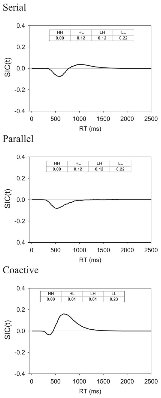
In Figure A2, we show the simulated SIC functions for the serial, parallel, and coactive models for cases in which the error rate on the LL stimulus is approximately .20. As can be seen, even for this relatively high error rate, the SIC signatures retain the shapes that are derived from the formal theorems. The same was true, of course, in all cases involving lower error rates. Finally, we conducted numerous other simulations involving parameter values that varied around the settings assumed in the representative simulations from Tables A1-A4 and observed the same pattern of results.

Appendix B

Multidimensional-Scaling Studies for the Color Stimuli

In this appendix, we describe the results of the similarity-scaling studies that we conducted for the color stimuli used in Experiment 2. Separate similarity-scaling studies were conducted for the Set 1 and Set 2 colors.

Method

Subjects

There were 15 subjects who participated in the Set 1 scaling study and 20 subjects who participated in the Set 2 scaling study. The subjects were undergraduates at Indiana University who received credit toward an introductory psychology course requirement.

Stimuli

The stimuli were the eight colors from Set 1 and the nine colors from Set 2 that were tested in Experiment 2. The colors were presented in pairs on the center of the computer screen against a white background. The members of each pair were separated by approximately 25 pixels.

Procedure

In both the Set 1 and Set 2 studies, the subjects were presented with 1 block of practice similarity-judgment trials (24 pairs for Set 1 and Set 2) and 3 blocks of experimental similarity judgments (56 pairs for Set 1 and 72 pairs for Set 2). Within each block, all distinct pairs of the stimuli were presented two times (28 pairs for Set 1 and 36 pairs for Set 2). On each trial, subjects rated the similarity of the pair of colors on a scale from 1 (very dissimilar) to 9 (very similar). The order of presentation of the pairs within each block, as well as the left–right placement of the members of each pair, were randomized anew for each subject and block.

Results

We analyzed the mean similarity judgments for the pairs of colors by using the standard Euclidean model from the ALSCAL program of the SPSS statistical package. For the Set 1 stimuli, the two-dimensional scaling solution yielded stress equal to .013 and accounted for 99.87% of the variance in the data. For the Set 2 stimuli, the two-dimensional scaling solution yielded stress equal to .036 and accounted for 98.90% of the variance in the data.

Figure B1.

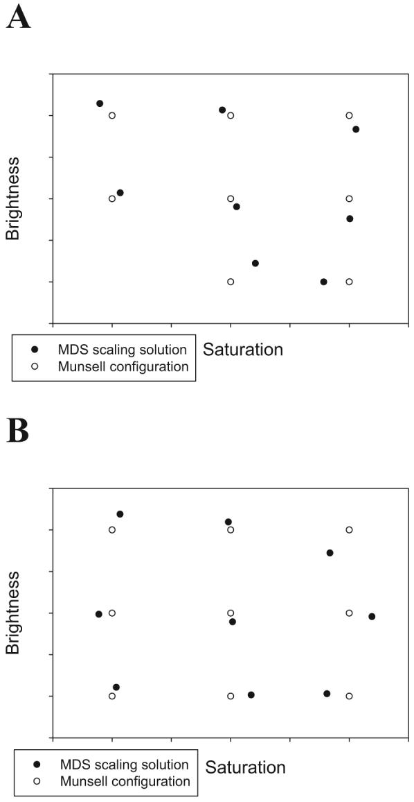
Multidimensional scaling (MDS) solutions for the color stimuli used in Experiment 2 along with the positions of the colors according to the Munsell system. A: Set 1 colors; B: Set 2 colors.

The scaling solutions are displayed graphically in Figure B1. It is evident from inspection that the intended 3 × 3 factorial structure of the experimental design is well approximated for each set.

References

- Ashby FG. Multidimensional models of perception and cognition. Erlbaum; Hillsdale, NJ: 1992. [Google Scholar]
- Ashby FG. A stochastic version of general recognition theory. Journal of Mathematical Psychology. 2000;44:310–329. doi: 10.1006/jmps.1998.1249. [DOI] [PubMed] [Google Scholar]
- Ashby FG, Maddox WT. A response time theory of separability and integrality in speeded classification. Journal of Mathematical Psychology. 1994;38:423–466. [Google Scholar]
- Ashby FG, Townsend JT. Varieties of perceptual independence. Psychological Review. 1986;93:154–179. [PubMed] [Google Scholar]
- Colonius H, Townsend JT. Activation-state representation of models for the redundant-signals-effect. In: Marley AAJ, editor. Choice, decision, and measurement: Essays in honor of R. Duncan Luce. Erlbaum; Mahwah, NJ: 1997. pp. 245–254. [Google Scholar]
- Diederich A, Colonius H. A further test of the superposition model for the redundant-signals effect in bimodal detection. Perception & Psychophysics. 1991;50:83–86. doi: 10.3758/bf03212207. [DOI] [PubMed] [Google Scholar]
- Dzhafarov EN. Conditionally selective dependence of random variables on external factors. Journal of Mathematical Psychology. 1999;43:123–157. doi: 10.1006/jmps.1998.1231. [DOI] [PubMed] [Google Scholar]
- Egeth HE, Dagenbach D. Parallel versus serial processing in visual search: Further evidence from subadditive effects of a visual quality. Journal of Experimental Psychology: Human Perception and Performance. 1991;17:550–559. doi: 10.1037//0096-1523.17.2.551. [DOI] [PubMed] [Google Scholar]
- Fific M. Emerging holistic properties at face value: Assessing characteristics of face perception. Indiana University; 2006. Unpublished doctoral thesis. [Google Scholar]
- Garner WR. The processing of information and structure. Erlbaum; Potomac, MD: 1974. [Google Scholar]
- Kantowitz BH. Human information processing: Tutorials in performance and cognition. Erlbaum; Hillsdale, NJ: 1974. [Google Scholar]
- Kruschke JK. Human category learning: Implications for back-propagation models. Connection Science. 1993;5:3–36. [Google Scholar]
- Lamberts K. Information accumulation theory of categorization. Psychological Review. 2000;107:227–260. doi: 10.1037/0033-295x.107.2.227. [DOI] [PubMed] [Google Scholar]
- Lockhead GR. Processing dimensional stimuli: A note. Psychological Review. 1972;79:410–419. doi: 10.1037/h0033129. [DOI] [PubMed] [Google Scholar]
- McKinley SC, Nosofsky RM. Selective attention and the formation of linear decision boundaries. Journal of Experimental Psychology: Human Perception and Performance. 1996;22:294–317. doi: 10.1037//0096-1523.22.2.294. [DOI] [PubMed] [Google Scholar]
- Miller J. Divided attention: Evidence for coactivation with redundant signals. Cognitive Psychology. 1982;14:247–279. doi: 10.1016/0010-0285(82)90010-x. [DOI] [PubMed] [Google Scholar]
- Mordkoff JT, Yantis S. An interactive race model of divided attention. Journal of Experimental Psychology: Human Perception and Performance. 1991;17:520–538. doi: 10.1037//0096-1523.17.2.520. [DOI] [PubMed] [Google Scholar]
- Nosofsky RM. Further tests of an exemplar-similarity approach to relating identification and categorization. Perception & Psychophysics. 1989;45:279–290. doi: 10.3758/bf03204942. [DOI] [PubMed] [Google Scholar]
- Nosofsky RM, Palmeri TJ. Learning to classify integral-dimension stimuli. Psychonomic Bulletin & Review. 1996;3:222–226. doi: 10.3758/BF03212422. [DOI] [PubMed] [Google Scholar]
- Nosofsky RM, Palmeri TJ. Comparing exemplar-retrieval and decision-bound models of speeded perceptual classification. Perception & Psychophysics. 1997a;59:1027–1048. doi: 10.3758/bf03205518. [DOI] [PubMed] [Google Scholar]
- Nosofsky RM, Palmeri TJ. An exemplar-based random walk model of speeded classification. Psychological Review. 1997b;104:266–300. doi: 10.1037/0033-295x.104.2.266. [DOI] [PubMed] [Google Scholar]
- Nosofsky RM, Stanton RD. Speeded classification in a probabilistic category structure: Contrasting exemplar-retrieval, decision-boundary, and prototype models. Journal of Experimental Psychology: Human Perception and Performance. 2005;31:608–629. doi: 10.1037/0096-1523.31.3.608. [DOI] [PubMed] [Google Scholar]
- Ratcliff R, Rouder JF. Modeling response times for two-choice decisions. Psychological Science. 1998;9:347–356. [Google Scholar]
- Schweickert R. Separable effects of factors on speed and accuracy: Memory scanning, lexical decision, and choice tasks. Psychological Bulletin. 1985;97:530–546. [PubMed] [Google Scholar]
- Schweickert R. Information, time, and the structure of mental events: A twenty-five year review. In: Meyer DE, Kornblum S, editors. Attention and performance XIV: Synergies in experimental psychology, artificial intelligence, and cognitive neuroscience. MIT Press; Cambridge, MA: 1992. pp. 535–566. [Google Scholar]
- Schweickert R, Giorgini M, Dzhafarov E. Selective influence and response time cumulative distribution functions in serial-parallel task networks. Journal of Mathematical Psychology. 2000;44:504–535. doi: 10.1006/jmps.1999.1268. [DOI] [PubMed] [Google Scholar]
- Shepard RN. Attention and the metric structure of the stimulus space. Journal of Mathematical Psychology. 1964;1:54–87. [Google Scholar]
- Shepard RN, Chang J. Stimulus generalization in the learning of classifications. Journal of Experimental Psychology. 1963;65:94–102. doi: 10.1037/h0043732. [DOI] [PubMed] [Google Scholar]
- Shepard RN, Hovland CI, Jenkins HM. Learning and memorization of classifications. (Whole No. 517).Psychological Monographs. 1961;75(13) [Google Scholar]
- Sternberg S. Memory scanning: Mental processes revealed by reaction-time experiments. American Scientist. 1969;4:421–457. [PubMed] [Google Scholar]
- Thomas RD. Processing time predictions of current models of perception in the classic additive factors paradigm. Journal of Mathematical Psychology. 2006;50:441–455. [Google Scholar]
- Townsend JT. Uncovering mental processes with factorial experiments. Journal of Mathematical Psychology. 1984;28:363–400. [Google Scholar]
- Townsend JT, Ashby FG. The stochastic modeling of elementary psychological processes. Cambridge University Press; Cambridge, England: 1983. [Google Scholar]
- Townsend JT, Nozawa G. Spatio-temporal properties of elementary perception: An investigation of parallel, serial, and coactive theories. Journal of Mathematical Psychology. 1995;39:321–359. [Google Scholar]
- Townsend JT, Nozawa G. Serial exhaustive models can violate the race model inequality: Implications for architecture and capacity. Psychological Review. 1997;104:595–602. [Google Scholar]
- Townsend JT, Schweickert R. Toward the trichotomy method of reaction times: Laying the foundation of stochastic mental networks. Journal of Mathematical Psychology. 1989;33:309–327. [Google Scholar]
- Townsend JT, Thomas RD. Stochastic dependencies in parallel and serial models: Effects on systems factorial interactions. Journal of Mathematical Psychology. 1994;38:1–34. [Google Scholar]
- Townsend JT, Wenger MJ. The serial-parallel dilemma: A case study in a linkage of theory and method. Psychonomic Bulletin & Review. 2004a;11:391–418. doi: 10.3758/bf03196588. [DOI] [PubMed] [Google Scholar]
- Townsend JT, Wenger MJ. A theory of interactive parallel processing: New capacity measures and predictions for a response time inequality series. Psychological Review. 2004b;111:1003–1035. doi: 10.1037/0033-295X.111.4.1003. [DOI] [PubMed] [Google Scholar]
- Wenger MJ, Townsend JT. Faces as Gestalt stimuli: Process characteristics. In: Wenger MJ, Townsend JT, editors. Computational, geometric, and process perspectives on facial cognition: Contexts and challenges. Erlbaum; Mahwah, NJ: 2001. pp. 229–284. [Google Scholar]
- Van Aken H. Munsell Conversion Software (Version 6.5.1) [Computer software] 2006 Retrieved January, 15, 2006, from http://livingstonmanor.net/Munsell/index.htm.