Statistical Mechanics and the Evolution of Polygenic Quantitative Traits

Abstract

The evolution of quantitative characters depends on the frequencies of the alleles involved, yet these frequencies cannot usually be measured. Previous groups have proposed an approximation to the dynamics of quantitative traits, based on an analogy with statistical mechanics. We present a modified version of that approach, which makes the analogy more precise and applies quite generally to describe the evolution of allele frequencies. We calculate explicitly how the macroscopic quantities (i.e., quantities that depend on the quantitative trait) depend on evolutionary forces, in a way that is independent of the microscopic details. We first show that the stationary distribution of allele frequencies under drift, selection, and mutation maximizes a certain measure of entropy, subject to constraints on the expectation of observable quantities. We then approximate the dynamical changes in these expectations, assuming that the distribution of allele frequencies always maximizes entropy, conditional on the expected values. When applied to directional selection on an additive trait, this gives a very good approximation to the evolution of the trait mean and the genetic variance, when the number of mutations per generation is sufficiently high (4Nμ > 1). We show how the method can be modified for small mutation rates (4Nμ → 0). We outline how this method describes epistatic interactions as, for example, with stabilizing selection.

PREDICTING the evolution of quantitative characters from first principles poses a formidable challenge. When multiple loci contribute to a quantitative character z, the effects of selection, mutation, and drift are difficult to predict from the observed values of the trait; this is true even in the simplest case of additive effects. The fundamental problem is that the distribution of the trait depends on the “microscopic details” of the system, namely the frequencies of the genotypes contributing to the trait. In an asexual population, long-term evolution depends on the fittest genotypes, which may currently be very rare. In sexual populations—the focus of this article—new phenotypes are generated by recombination in a way that depends on their genetic basis. If selection is not too strong, we can assume Hardy–Weinberg proportions and linkage equilibrium (HWLE): this is a substantial simplification, which we make throughout. Even then, however, we must still know all the allele frequencies, and the effects of all the alleles on the trait, to predict the evolution of a polygenic trait. In this article, we seek to predict the evolution of quantitative traits without following all the hidden variables (i.e., the allele frequencies) that determine its course.

For this purpose, several simplifications have been proposed. The central equation in quantitative genetics is that the rate of change of the trait mean equals the product of the selection gradient and the additive genetic variance (Lande 1976). This simple prediction can be surprisingly accurate, since the genetic variance often remains roughly constant for some tens of generations (Falconer and Mackay 1996; Barton and Keightley 2002). However, we have no general understanding of how the genetic variance evolves or, indeed, what processes are responsible for maintaining it (Bürger et al. 1989; Falconer and Mackay 1996; Barton and Keightley 2002). Even if we take the simplest view, that variation is maintained by the opposition between mutation and selection, the long-term dynamics of the genetic variance still depend on the detailed distribution of effects of mutations.

Lande (1976), following Kimura (1965), approximated the distribution of allelic effects at each locus as a Gaussian distribution. However, this is accurate only when many alleles are available at each locus and when mutation rates are extremely high (Turelli 1984). Barton and Turelli (1987) assumed that loci are close to fixation, but again this approximation has limited application: in particular, it cannot apply when one allele substitutes for another. Some progress has been made by describing a polygenic system by the moments of the trait distribution (Barton 1986; Barton and Turelli 1987, 1991; Turelli and Barton 1990). For additive traits, a closely related description in terms of the cumulants is a more natural way to represent the effects of selection (Bürger 1991, 1993; Turelli and Barton 1994; Rattray and Shapiro 2001). These transformations are exact and quite general: they provide a natural description of selection and recombination and extend to include the dynamics of linkage disequilibria as well as allele frequencies. A moment-based description provides a general framework for exact analysis of models with a small number of genes and for approximating the effects of indirect selection (Barton 1986; Barton and Turelli 1987; Lenormand and Otto 2000; Kirkpatrick et al. 2002; Roze and Barton 2006); for some problems, simply truncating the higher moments or cumulants can give a good approximation (Turelli and Barton 1990; Rouzine et al. 2007). However, results are sensitive to the choice of approximation for higher moments, and so the approximation is to this extent arbitrary. The equations must be truncated “by hand,” guided by mathematical tractability rather than biological accuracy.

The fundamental problem is to find a way to approximate the “hidden variables” (in this context, the allele frequencies), but we cannot hope to do this in complete generality. Even with simple directional selection on a trait, the pattern of allele frequencies depends on the frequencies of favorable alleles that may be extremely rare and that will take ∼ generations to reach appreciable frequency. Thus, undetectably rare alleles can shape future evolution, without much affecting the current state. Figure 1 shows an example where the trait mean changes as three alleles sweep to fixation at different times and rates. By choosing initial frequencies and allelic effects appropriately, we could produce arbitrary patterns of trait evolution. We can hope to make progress only in situations where the underlying allele frequencies can be averaged over some known distribution, rather than taking arbitrary values.

Figure 1.—

The frequency of favorable alleles at three loci (left) and the mean of an additive trait, (right). Initial frequencies are 10⁻⁵, 10⁻⁶, 10⁻⁷, and effects on the trait are 1, 2, , so that ; the selection gradient is β = 0.01 (i.e., fitness is ).

Despite this fundamental difficulty, progress can be made in two ways. First, we can include random drift and follow the distribution of allele frequencies, rather than the deterministic evolution of a single population. Then, we can hope that the distribution of allele frequencies, conditional on the observed trait values, will explore the space of possible states in a predictable way. Second, we can allow selection to act only on the observed traits and assume that the distribution of allele frequencies spreads out to follow the stationary distribution generated by such selection. That makes it much harder (and perhaps impossible) for populations to evolve into an arbitrary state with unpredictable and idiosyncratic properties. There is an analogy here with classical thermodynamics, in which molecules might start in a special state, such that after some time they concentrate in a surprising way: all the gas might rush to one corner, for example. However, if all states with the same energy are equally likely, this is extremely improbable.

An approach along these lines was proposed by Prügel-Bennett and Shapiro (1994, 1997), Rattray (1995), and Prügel-Bennett (1997), as a general framework for approximating the dynamics of polygenic systems. Prügel-Bennett and Shapiro (1994, 1997), Rattray (1995), and Prügel-Bennett (1997) drew on analogies with statistical physics to propose an elegant approach to approximating polygenic systems. The distribution of microstates is chosen as that which maximizes an entropy measure (see also van Nimwegen and Crutchfield 2000; Prügel-Bennett 2001; Rogers 2003). Prügel-Bennett and Shapiro (1994, 1997), Rattray (1995), and Prügel-Bennett (1997) define an entropy that is maximized by a multinomial allele frequency distribution, which is sharply peaked around equal allele frequencies. Thus, the procedure is to assume maximum polymorphism, subject to constraints on the trait distribution. This averaging yields a generating function from which observables (e.g., mean values, variance, and higher moments, as well as correlations) can be obtained. This leads to good approximations for a variety of problems, including multiplicative selection, pairwise epistasis, and stabilizing selection (Rattray 1995); it describes the dynamics of an arbitrary number of observable variables and provides a consistent way to deal with hidden microscopic variables.

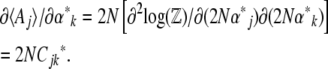
In this article, we use procedures analogous to statistical thermodynamics, but adapted to population genetics. First, we use an information entropy measure, S_H, which is derived from population genetic considerations and ensures an exact solution at statistical equilibrium. This measure, which is proportional to the quantity H, defined by Boltzmann (1872), was proposed by Iwasa (1988) and independently by Sella and Hirsh (2005); see N. H. Barton and J. B. Coe (unpublished data). Second, we choose to follow a set of observable quantities that includes all those acted on directly by mutation and selection. This reveals a natural correspondence between the observables and the evolutionary forces that act on them, which is analogous to extensive and intensive variables in thermodynamics (N. H. Barton and J. B. Coe, unpublished data). These two innovations allow us to set out the method in a very general way.

Throughout, we make the usual approximations of population genetics, that populations are at HWLE and that drift, mutation, and selection are weak. Linkage equilibrium is justified if selection and drift are not only weak () but also weak relative to recombination (). We also assume only two alleles at each locus. These assumptions allow us to describe populations solely in terms of allele frequencies at n loci and to use the continuous-time diffusion approximation.

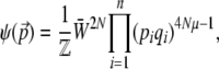
We begin by analyzing the stationary distribution, showing the analogy with thermodynamics. Iwasa (1988) showed that the free fitness, which is the sum of the log mean fitness and the information entropy S_H (), always increases through time and reaches a maximum at the classic stationary distribution of allele frequencies under mutation, selection, and drift,

(1)

where p_i (i = 1,…, n) are the allele frequencies at n loci, q_i = 1 − p_i, N is the number of diploid individuals, is the mean fitness, and μ is the mutation rate (Wright 1937). The normalizing constant plays a key role; it is analogous to the partition function in statistical mechanics and acts as a generating function for the quantities of interest, in the sense that its derivatives give the expectations of the macroscopic quantities (Barton 1989). We then show how the rates of change of expectations of observable quantities can be approximated by averaging over this stationary distribution ψ. The crucial assumption here is that the distribution of allele frequencies always has the form of Equation 1. This is accurate provided that the system evolves as a result of slow changes in the parameters, so that it has time to approach the stationary state. By analogy with thermodynamics, such changes are termed reversible (Ao 2008; N. H. Barton and J. B. Coe, unpublished data).

After setting out the method in a general way, we apply it to directional selection on an additive trait. In this simple case, we can give closed-form expressions for the generating function and hence for observables such as the expectations of the trait mean, genotypic variance, genetic variability, and so on. We then show that our approximation to the allele frequency distribution gives a good approximation to the dynamical change in the trait distribution, even when selection changes abruptly. However, the method works only for high mutation rates (4Nμ > 1) and breaks down when 4Nμ < 1. Nevertheless, we show how the method can be adapted to the case where 4Nμ is small. Finally, we outline the application to cases such as stabilizing selection, where there are epistatic interactions for fitness.

GENERAL ANALYSIS

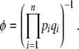
Defining entropy:

The key concept is of an entropy, S_H, which measures the deviation of the population from a base distribution φ—in this case, the density under drift alone. Entropy always increases as the population converges toward φ under drift. With selection and mutation, a “free energy”—the sum of the entropy and a potential function—always increases (Iwasa 1988). We show that the stationary distribution maximizes S_H subject to constraints of the expected value of a set of observable quantities. Thus, the dynamics of these quantities can be approximated by assuming that the entropy is always maximized, conditioned on their values.

There is a wide range of definitions, interpretations, and generalizations of entropy (e.g., Renyi 1961; Wehrl 1978; Tsallis 1988); these have been applied to biological systems in various ways. Iwasa (1988) introduced the concept of entropy into population genetics, for a diallelic system of one locus under reversible mutation and with arbitrary selection; he also considered a phenotypic model of quantitative trait evolution. Iwasa (1988) used an information entropy, also known as a relative entropy (Gzyl 1995, Chap. 3; Georgii 2003), and defined as

(2)

This is a function of the probability distribution of allele frequencies, ψ, that evaluates the average entropy of a function with respect to a given base distribution, φ, integrated over all possible allele frequencies, denoted by . It can be thought of as the expected log-likelihood of φ, given samples drawn from a distribution ψ; it has a maximum at ψ = φ, when S_H[φ] = 0. We denote it by a subscript H because it is essentially the same as the measure introduced by Boltzmann (1872) in his H-theorem.

The variation of S_H with respect to small changes in ψ is

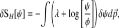(3)

where λ is a Lagrange multiplier associated with the normalization condition (N. H. Barton and J. B. Coe, unpublished data) (see supplemental information A). Note that because ψ is normalized, = 0. With no constraints other than this normalization, setting δS_H = 0 implies that the entropy is at an extreme only if ψ = φ; this is a unique maximum.

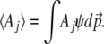
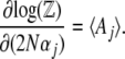
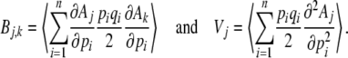
We are interested in a set of observable quantities, A_j, which are functions of the allele frequencies in a population. These might, for example, describe the distribution of a quantitative trait—for example, its mean and variance. We need to find the distribution of allele frequencies, ψ, that maximizes the entropy, S_H[ψ], given constraints on the expected values of these observables, :

(4)

With these constraints, the extremum of Equation 3 is calculated by including the Lagrange multipliers associated with the A_j's, defined for convenience as −2Nα_j:

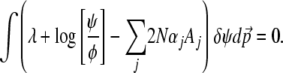(5)

At the extremum, the term in parentheses should be zero. This implies that the distribution that maximizes entropy, subject to constraints, is the Boltzmann distribution

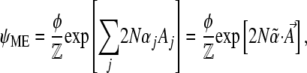(6)

where we have expressed the Lagrange multiplier λ as = exp(λ) and choose to normalize the distribution. We show later that is a generating function for the moments of the observables, A_j. It will play a major role in our calculations:

(7)

We show that under directional selection and mutation the α_j can be identified with the set of selection coefficients and mutation rates and the A_j with the quantities on which selection and mutation act (e.g., trait mean and genetic variability). The potential function 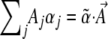consists of the log-mean fitness, , plus a term representing the effect of mutation, 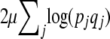. Then, Equation 6 gives the classical stationary density of Equation 1. (Note that although must equal the potential function, which includes all evolutionary processes, apart from drift, we still have some freedom to separate this into components in a variety of ways. For example, directional selection on a set of traits could be represented by almost any linear basis. Nevertheless, there will usually be a natural set of components that represent different evolutionary processes. In addition, we are free to include additional observables that are not necessarily under selection, and so have α_i = 0. These extra degrees of freedom will improve the accuracy of our dynamical approximations.)

Note that there is an alternative measure of entropy, S_Ω, defined by the log density of states that are consistent with macroscopic variables (Barton 1989). N. H. Barton and J. B. Coe (unpublished data) discuss the relation between S_Ω and S_H and show that these two measures converge when the distribution clusters close to its expectation.

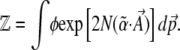
The generating function, Z:

The normalizing constant , which is a function of , acts as a generating function for quantities of interest. Differentiating with respect to (w.r.t.) we find that

(8)

Differentiating w.r.t. population size,

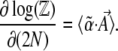(9)

Differentiating again w.r.t. the gives the covariance between fluctuations in the :

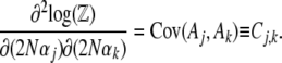(10)

This covariance matrix, which we denote C, plays an important role in the dynamical approximation (Le Bellac et al. 2004, p. 64).

Analyzing the dynamics:

As the system moves away from stationarity, it will not in general follow precisely the distribution that maximizes entropy. [This can be seen by substituting the maximum entropy distribution from Equation 6 with time-varying parameters as a trial solution to the diffusion equation]. However, the distribution of microscopic variables may nevertheless stay close to a maximum entropy distribution (Nicolis and Prigogine 1977; De Groot and Mazur 1984; Goldstein and Lebowitz 2004). Our key assumption is that the macroscopic variables change slowly enough that the system is always close to a local equilibrium.

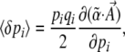
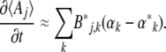
We show that the Lagrange multipliers, , correspond to forces that act on the observables, : directional selection acts on the trait mean, mutation on a measure of genetic diversity U (see below), and so on. Crucially, we assume that changes occur solely through changes in the parameters ; arbitrary perturbations that act directly on the allele frequencies could have arbitrary effects (as, for example, in Figure 1).

Assume that changes in allele frequency are determined by a potential function , which can be written as a sum of components α_kA_k. [In physics, energy acts as a potential; in population genetics, mean fitness plays an analogous role; it defines an adaptive landscape such that allele frequencies and their means change at rates proportional to the fitness gradient (Wright 1967; Lande 1976).] Our method works only for systems whose dynamics can be described by a potential in this way (although see Ao 2008). In an infinitesimal time δt, the mean and mean-square changes are

(11a)

(11b)

(11c)

The first equation, for , is just Wright's (1937) formula for selection, modified to include mutation. The variance of allele frequency fluctuations, , is the standard formula for random drift. Under the diffusion approximation, this leads to the stationary distribution of Equation 1, provided that the base distribution is defined as

(12)

Under the diffusion approximation, the rate of change of is

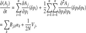(13)

where

(14)

This relationship is exact, provided that the matrix B and the vector V are evaluated at the current distribution of allele frequencies. Equation 13 can also be derived directly, by making a diffusion approximation to multivariate observables, where the deterministic terms are 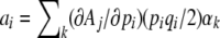, and the diffusion terms are 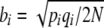(Ewens 1979; Gardiner 2004). If our system is described by only one observable, we directly recover the formula derived by Ewens (1979, pp. 136–137).

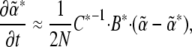
The local equilibrium approximation:

In general, as the system moves away from stationarity, it will not precisely follow the distribution that maximizes entropy. However, the distribution of microscopic variables may nevertheless stay close to a maximum entropy distribution if the macroscopic variables change slowly enough such that the system remains close to a local equilibrium at all times (Prigogine 1949; Klein and Prigogine 1953; Nicolis and Prigogine 1977; De Groot and Mazur 1984; Goldstein and Lebowitz 2004).

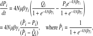
We now approximate B_j,k and V_j by B*, V_j*, assuming the distribution in Equation 6 is evaluated at . We know that at the stationary state, under parameters , expectations are constant, and so from Equation 13, 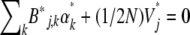. Therefore

(15)

The matrix B_j,k is closely related to the additive genetic covariance matrix. Making the link with quantitative genetics is not quite straightforward, because the A_j are arbitrary functions of the allele frequencies and need not be the means of actual traits carried by individuals. Nevertheless, if we do regard them as the means of some quantity, then ∂A_j/∂p_i is twice the average effect of alleles at locus i. [Since we assume HWLE, average effect is equal to average excess (Falconer and Mackay 1996)]. Therefore, B_j,k is the expected additive genetic covariance between A_j and A_k, the expectation being taken over the distribution of allele frequencies. Moreover, if the α_k contribute to the log-mean fitness (rather than to the component of the potential that describes mutation), then they can be interpreted as selection gradients in the usual way. Equation 15 thus gives the rates of change of the expected trait means as the product of the expected additive genetic covariance, and the difference between the actual selection gradient, α_k, and the gradient that would give stationarity at the current expectations, . This interpretation becomes clearer when we consider specific examples, below.

In the theory of nonequilibrium thermodynamics, equations similar to Equation 15 are called phenomenological equations (van Kampen 1957; De Groot and Mazur 1984, Chap. IV). They were first postulated as approximations to processes that are close to equilibrium. In such cases, the variables α* represent the deviation from an equilibrium defined by α. These equations are valid as long as a local equilibrium exists, and (as suggested by Equation 13) it holds in general that B_k,j = B_j,k (Onsager 1931; Prigogine 1949).

For theoretical purposes, we can follow either the expectations themselves or the parameters that would give those expectations at stationarity. In numerical calculations, the latter is more convenient, because that avoids calculating the from the (a tricky inverse problem). The rates of change of the are related to the rates of change of the via the matrix . Now, since 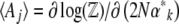, we have

Thus, the relation between the and the is via the covariance of fluctuations, (Equation 10). In matrix notation (equivalent to De Groot and Mazur 1984, p. 36),

(16)

where C is the matrix of covariances of fluctuations in the , and B is analogous to the additive genetic covariance matrix.

Both of these are evaluated at the stationary distribution defined by . For given , we find the by integrating using the density in Equation 6, or by application of Equation 8.

DIRECTIONAL SELECTION, MUTATION, AND DRIFT

Analysis:

The stationary distribution:

We now apply this method to a quantitative trait under directional selection, mutation, and drift. We first define a measure of genetic variability (N. H. Barton and J. B. Coe, unpublished data),

(17)

which is 2n times the log-geometric mean heterozygosity across loci (plus a constant); n is the number of loci. The rate of change of p_i due to symmetric mutation is , as required by Equation 11a. Under our assumption of linkage equilibrium, the rate of change of p_i due to selection is (Equation 11a). The log mean fitness, , is a natural potential for the system and will be expressed as a sum of components , where the are a set of selection coefficients. We deal with the very simplest case of exponential (directional) selection, but note that the derivation applies to any form of selection for which a potential function can be defined—most obviously, the case where genotypes have fixed fitnesses (see supplemental information A and D). If individuals with trait value z have fitness e^βz, then to leading order in β, the mean fitness is . Wright's equilibrium density can then be written in the form of Equation 6, with and :

(18)

Thus, the stationary distribution under mutation, selection, and random drift is given by maximizing the entropy subject to constraints on the expected genetic diversity and the expected trait mean . The entropy is defined by Equation 2, with baseline distribution . Then, Equation 18 is the stationary distribution and is equal to Equation 1.

We have shown that a population evolving under mutation, multiplicative selection, and drift will converge to a stationary distribution that has maximum entropy, S_H, given the expected trait mean and genetic diversity. As we will see below, other forms of selection can be represented by introducing other observables. Each constrained observable will be conjugated with a natural variable: in this example, the expected mean corresponds to the strength of directional selection β, and the expected diversity to the mutation rate μ. Information about the full distribution of the observables is contained in the normalizing constant , which is a generating function that depends only on the natural variables α_j. In the next section, we calculate an explicit expression for it.

The generating function for an additive trait:

We have not yet made any assumptions about the genetic basis of the trait, z; in general, there might be arbitrary dominance and epistasis. We now assume that it is additive, with locus i having effect γ_i,

(19)

where X_i and X_i* represent the allelic states (labeled 0 or 1) of the two copies of each of the n loci. With additivity, exponential selection on the trait corresponds to multiplicative selection on the underlying loci. If we average over the population, where p_i represents the frequency of the X_i = 1 allele, and q_i = 1 − p_i, then the mean and genetic variance are

(20)

More than two alleles could be allowed, but only for special mutation rates that give detailed balance (that is, there must be no flux of probability in the stationary state).

The normalization function can now be calculated explicitly, using Equation 7. In this simple case of directional selection on an additive trait, the integrand separates out as a product over allele frequencies, and so

(21a)

(21b)

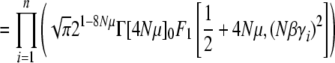(21c)

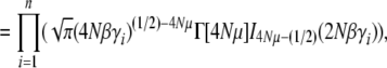(21d)

where Γ(·) and ₀F₁(·, ·) are the gamma and the regularized confluent hypergeometric functions, respectively. We have also given an equivalent form, in terms of the modified Bessel function of order ν, I_ν(·).

Finding the expectations 〈U〉,〈z̄〉:

The expectations, variances, and covariances of and U can be calculated either by direct integration or by taking derivatives of log() w.r.t. β and μ (Equations 8 and 10). Explicit formulas are given in supplemental information A.

Figure 2 shows how the expected values change for a range of mutation rates and selection pressures, for a population of individuals with n loci of equal effect, γ_i = 1. As selection becomes strong relative to mutation, the allele X = 1 tends to fixation, and tends to n (top right of Figure 2). As mutation becomes strong relative to drift, allele frequencies tend to , and tends to zero (top left of Figure 2). The expected diversity, , increases with mutation rate (bottom left of Figure 2) and decreases slightly with the strength of selection (bottom right of Figure 2). Figure 2 compares the diffusion approximation with the Wright–Fisher model for N = 100. There is close agreement for for all 4Nμ and for when 4Nμ > 1. In the discrete model, must be calculated excluding the fixed classes, since U would otherwise be infinite. This has negligible effect when 4Nμ > 1 because fixation is unlikely. However, when 4Nμ < 1, there is a substantial probability of being fixed, even when fixed classes must be dropped. Thus, depends on population size and differs substantially from the diffusion approximation (compare bottom series of dots with bottom curve in Figure 2, bottom right). The stationary density is still close to the diffusion approximation for polymorphic classes, and so for very large N, when the probability of actually being fixed becomes small , in the discrete Wright–Fisher model does converge to the diffusion approximation. However, for population sizes in the hundreds, there is still a very large discrepancy. We consider the implications of small 4Nμ for the maximum entropy method below.

Figure 2.—

Dependence of on Nμ, Nβ. The solid curves show the diffusion approximation, while the dots show exact values for the Wright–Fisher model with N = 100. The plots against Nμ (left column) show Nβ = 0.1, 1, 10; those against Nβ (right column) show Nμ = 0.1, 1, 10. Agreement between discrete and continuous models is close for and for 4Nμ > 1, but the diffusion approximation fails to predict when 4Nμ = 0.1 (bottom series of dots at bottom right). (For the discrete model, is calculated omitting fixed classes.)

For an additive trait, and equal allelic effects, the distribution of allele frequencies is the same at each locus, and so this simple case is essentially a single-locus analysis. However, this is no longer the case when we allow unequal allelic effects; more generally, if there is epistasis for fitness, the allele frequency distributions at each locus are no longer independent, and if there is epistasis for the trait, we can no longer treat macroscopic variables as sums over loci.

Covariances of fluctuations, C, and additive genetic variance, B:

To approximate the dynamics, we need the covariances of fluctuations, C, and the additive genetic covariance, B, defined above. The matrix C, which gives the variances and covariance of U and , is calculated by taking derivatives of the generating function (Equation 10; supplemental information A, Equations A3–A6).

The additive genetic covariance matrix B is defined in Equation 13, in terms of the derivatives ∂A_j/∂p_i. For the observables , these are . Using the relation ,

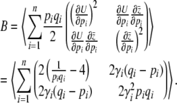(22)

Note that 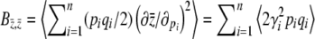is just the expected genetic variance for the trait z, , consistent with our interpretation of B as a genetic covariance matrix. For this model, B has a simple form:

(23)

Remarkably, B depends only on and not directly on the distribution of allelic effects, γ. Note that the expected genetic variance = , even with unequal allelic effects. This can be understood by seeing that the rates of change of due to mutation, −2, and due to selection, , must balance at statistical equilibrium. In the limit where selection becomes weak, both and Nβ tend to zero, and the expected genetic variance tends to a definite limit.

The coefficient B_U,U includes the expectation of , which diverges when 4Nμ < 1. Because the rate of change depends on (Equation 23), that implies that μ* must be held fixed at its actual value (i.e., μ* = μ). In effect, therefore, can no longer be included in the approximation. We discuss the implications of this constraint below.

Approximating the dynamics:

Evolution of the expectations:

We can now use Equation 15 to approximate the rates of change of the expectations :

(24)

These equations are proportional to the difference between the actual parameters {μ, β} and the parameters that would give a stationary distribution with the current expectations, . To iterate these recursions, we would need to find from , which is troublesome. It is more straightforward to work with the rates of change of , which are found by multiplying the rates of change of the expectations (Equation 24) by the inverse of the covariance of fluctuations, C (see Equation 16 and supplemental information A, Equation A6). However, because C depends on the allelic effects in a complex way (see supplemental information A, Equations A3–A5), the full dynamics do depend on the distribution of allelic effects, γ_i.

In the following sections we test the accuracy of this local equilibrium approximation against two situations: an abrupt change in β or μ or a sinusoidal change in μ or β. An abrupt change seems the strongest test of our approximation, while a sinusoidal change allows us to find how the accuracy of the approximation decreases as changes become faster. For the moment, we focus on high numbers of mutations (4Nμ > 1). We begin by considering the case of equal effects, where the distributions at all loci are the same. We also discuss results for the case where most loci have small effect, but some have large effect: the patterns are similar to the symmetric case of equal effects, and so we detail them in supplemental information C. Throughout, we compare the approximation with numerical solutions of the diffusion equation: these are close to solutions of the discrete Wright–Fisher model provided that 4Nμ > 1 (Figure 3).

Figure 3.—

(Top) Calculation of genetic variability (left) and trait mean (right) and over time, with Nμ = 0.6 as Nβ changes from −2 to +2 at time t = 0. The horizontal lines show the stationary values. The solid curves show the approximation, and the dashed curves show numerical solutions to the diffusion equation; these are not distinguishable on this scale. (Bottom) Changes over time in the parameters μ* (left) and β* (right), calculated using the approximation of Equation 16. Time is scaled to 2N generations.

Equal allelic effects:

If all loci have equal effects on the trait, and if selection acts only on the trait, and not on the individual genotypes, then under directional selection the distribution of allele frequencies will be the same at each locus and will be independent across loci. Thus, we need follow only a single distribution, whose time evolution is given either by numerical solution of the diffusion equation or as an expansion of eigenvectors (Crow and Kimura 1970, p. 396). However, the maximum entropy approximation is still nontrivial, even in this highly symmetric case, since it approximates the full distribution by a few degrees of freedom, such as {, }. Also, note that with other forms of selection, the allele frequency distribution is not independent across loci: for example, with stabilizing selection populations cluster around states where the sum of allele frequencies is close to the optimum.

Abrupt change in Nβ:

First, assume that a system is at equilibrium with evolutionary forces β₀ and μ₀. These forces are then abruptly changed to new values β and μ, and the system moves toward its new stationary state. Figure 3 shows that for moderately high mutation rates (Nμ = 0.6), and for an abrupt change of selection from Nβ = −2 to +2, the approximation is extremely accurate, as compared with the numerical solutions of the diffusion equation. The expected genetic diversity, , increases as the allele frequencies pass through intermediate values, but returns to its original value as moves from −2 to +2 (top left). This transient increase in diversity is mainly due to the change in mean allele frequencies: there is only a small transient change in μ* (bottom left). The distribution of allele frequencies predicted by the approximation is always close to the actual distribution (not shown).

For a lower mutation rate of Nμ = 0.3, close to the critical value of , the effective mutation rate hardly changes: it is held close to the actual value of Nμ = 0.3 (Figure 4, bottom left). The approximation is still accurate, although there is an appreciable discrepancy in (Figure 4, top left). For a still lower mutation rate of Nμ = 0.1, below the threshold where B_U,U diverges, μ* must necessarily be held equal to the current mutation rate, μ (Figure 5, top left). Then, there is a poor fit to the transient increase in expected diversity, , but the dynamical approximation to remains accurate (Figure 5, top right). (Because μ* must be held fixed at its actual value when 4Nμ < 1, is not now included in the approximation, which therefore now depends on fitting one variable, rather than two.)

Figure 4.—

The accuracy of the approximation for Nμ = 0.3. Nβ changes from −0.7 to +0.7 at time t = 0. Otherwise, details are as in Figure 3.

Figure 5.—

The accuracy of the approximation for Nμ = 0.1. Nβ changes from −0.7 to +0.7 at time t = 0. The effective mutation rate, Nμ*, is held fixed at Nμ (bottom left). Otherwise, details are as in Figure 3.

Abrupt change in Nμ:

Figure 6 shows the effects of an abrupt change in mutation rate from Nμ = 0.3 to 1. Here, the approximation does poorly when mutation rate increases abruptly, even when 4Nμ is always >1 (Figure 6, left side). It does perform better when the mutation rate decreases abruptly, however (t > 5 in Figure 6).

Figure 6.—

The mutation rate increases abruptly from Nμ = 0.3 to Nμ = 1 at t = 0 and then changes back at t = 5; throughout, Nβ = 1. The horizontal dashed lines show values at the stationary states, the dashed curves show numerical solutions of the diffusion equation, and the solid curves in the top row show the approximation.

Fluctuating selection:

As well as examining the effects of an abrupt change in selection, we have also looked at the effects of oscillating selection. If fluctuations are sufficiently slow, then the maximum entropy approximation converges to the exact solution. At the other extreme, when fluctuations are rapid, populations experience an average selective force and behave as if there was a constant selective pressure. The approximation is accurate over the whole range of fluctuation frequencies (supplemental information B).

Unequal allelic effects:

So far, we have assumed equal allelic effects. This ensures that the allele frequency distribution is the same at each locus, so that we are essentially analyzing a single-locus problem. This is not entirely trivial, since we are approximating the full allele frequency distribution by two variables, . However, we now turn to the more challenging case of unequal allelic effects at n loci: now, we are summarizing n distinct distributions by two variables. We do, however, assume that the allelic effects are known.

We draw allelic effects at 10 loci from a gamma distribution, with mean 1 and standard deviation :

(25)

The maximum range of the trait is , and the maximum genetic variance is 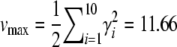. Twenty-five percent of this is contributed by the locus of largest effect, and 54% by the largest three loci.

Figure 7 shows the response of the mean and the genetic variance, as selection changes from Nβ = −2 to +2, with Nμ = 0.3 throughout: the approximation matches well. There is a transient increase in the genetic variance as allele frequencies pass through intermediate values. In Figure 7, the shift is by 3.08 genetic standard deviations.

Figure 7.—

The accuracy of the approximation with unequal allelic effects, γ, given by Equation 25. Nβ changes from −2 to +2 at time t = 0; Nμ = 0.5 throughout. Otherwise, details are as in Figure 3.

In supplemental information C, we show how the accuracy of the approximations diminishes as Nμ approaches , in a similar way to Figures 3–5.

LOW MUTATION RATES: 4Nμ < 1

Failure of the maximum entropy approximation:

When the number of mutations produced per generation is small (4Nμ < 1), populations are likely to be close to fixation. The diffusion approximation still works surprisingly well: it predicts the allele frequency distribution accurately even adjacent to the boundaries 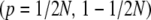. The maximum entropy approximation also makes accurate predictions for the change in trait mean, provided that the mutation rate is kept fixed (Figure 5, top right). However, the approximation does not allow changes in μ* when 4Nμ < 1. Formally, the coefficient B_U,U (Equation 23) diverges, which implies that the effective mutation rate must always be held equal to the actual mutation rate . Thus we lose 1 d.f. from the dynamics. What causes this pathological behavior?

The key point is that near the boundary, the allele frequency distribution changes on a much faster timescale than in the center: the characteristic timescale of random drift is determined by the number of copies of the allele in question. Thus, the shape of the distribution at the center and the shape at the edge are uncoupled, so that it may be impossible to adequately approximate the whole distribution as being close to the stationary state. Near the boundaries, selection is negligibly slow relative to mutation and drift, and the allele frequency distribution rapidly takes the form p^4Nμ−1, even while the bulk of the distribution remains unchanged (Figure 8). For example, suppose that 4Nμ changes from <1 to >1. The density at the boundaries immediately falls to zero, and the distribution takes on a two-peaked shape that cannot be approximated by any of the family of stationary distributions. Conversely, when 4Nμ falls below the threshold, small singularities immediately develop at the boundaries, representing fixed populations, but it takes a long time for the bulk of the population to approach fixation. This asymmetry explains why the maximum entropy approximation is much more accurate when 4Nμ falls than when it rises (Figure 6, t > 5).

Figure 8.—

Failure of the maximum entropic distribution of allele frequencies at the borders for changing mutation rates. Top panel, dotted curves: the genuine distribution, given by the diffusion equation; solid curves show the maximum entropic distribution. The bulk of the distributions is well approximated initially (curves toward the right; t = 0) and close to equilibrium (bell-shaped curves; t = 5). Bottom left panel: the max-entropic distribution at different times (from t = 0 to t = 5, top to bottom) near the edge p = 1 incorrectly predicts that there is no fixation, compared the diffusion equation solutions at different times (from t = 0 to t = 5, top to bottom) near the edge p = 1, which shows that some genotype fixes (bottom right panel). Numerics are as in Figure 6.

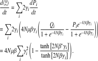
We can gain some insight by analyzing the limit of 4Nμ → 0, when populations are almost always fixed for one of the 2ⁿ genotypes. With directional selection, the probability of fixation of one or the other allele is independent across loci and equals 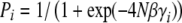, where γ_i is the effect of alleles at the ith locus. Populations will jump from fixation for “0” to “1” as a result of the fixation of favorable mutations, at a rate 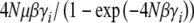, and in the opposite direction due to fixation of deleterious alleles, at a rate that is slower by a factor . In this simple case, it is easy to write down the dynamics at each locus,

(26)

noting that this does have a sensible limit as β → 0: ∂_tP = μ(1 − 2P), which is correct for neutral alleles. The trait mean changes as

(27)

The maximum entropy approximation simplifies the problem by assuming that the P_i always follow a stationary distribution, determined by a single parameter β*, with 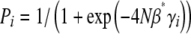. Thus, provided we know the allelic effects, we can deduce the P_i from the observed , without knowing the distribution at the n loci individually. From Equation 24, assuming that μ = μ*, we have

(28)

This can be understood by seeing that at equilibrium, selection must balance mutation, so that at each locus if the P_i follow a stationary distribution with parameter β*. The rate of change of the trait mean is

equal to Equation 28.

It is easy to show that the maximum entropy approximation, Equation 28, converges to the exact solution, Equation 27, for small Nβγ_i; this is confirmed by Figure 9, for Nβ = 0.2, in an example with equal effects, γ_i = 1. However, for stronger selection (Nβ = 2, thick lines in Figure 9), the maximum entropy approximation underestimates the initial rate of increase. That is because the approximation is that the initial state, in which P_i = 0.02 at all loci, is caused by strong selection against the 1 allele; such selection would necessarily cause low standing variation, and so the prediction is for a slow response when the direction of selection is reversed. However, as soon as selection is reversed, populations fix new favorable mutations at a rate that is independent of the previous standing variation. Thus, the method that led to Equation 24, which was developed for polymorphic populations, fails as 4Nμ → 0.

Figure 9.—

Comparison between the exact solution (Equation 27) and the maximum entropy approximation (Equation 28), in the limit of low mutation rates (4Nμ → 0). Initially, the probability that a locus is fixed for the “1” allele is P = 0.02 at all loci, so that ; all alleles have effect γ = 1. Selection Nβ = 0.2 or Nβ = 2 is then applied, and the trait mean shifts to a new equilibrium, in which a fraction P = 1/(1 + exp(−4Nβ)) of loci are fixed for the 1 allele. When selection is weak (Nβ = 0.2), the maximum entropy approximation is barely distinguishable from the exact solution. However, when selection is strong (Nβ = 2), the maximum entropy approximation (dashed lines) underestimates the initial rate of change.

Maximum entropy for 4Nμ → 0:

When mutation is rare, populations are almost always fixed for one of the 2ⁿ genotypes, and an ensemble of populations (or equivalently, the probability distribution of a single population) evolves as a result of jumps between genotypes, mediated by fixation of single mutations. The stationary distribution is proportional to , multiplied by a factor that reflects the pattern of mutation rates (Iwasa 1988; Sella and Hirsh 2005); this can be derived as the limit of Equation 1 for small 4Nμ (N. H. Barton and J. B. Coe, unpublished data). We can go further and apply the maximum entropy method to this process. This gives an approximation for the dynamics of macroscopic quantities such as , so that we do not need to follow the full distribution across the 2ⁿ genotypes. In the simplest case of directional selection on an additive trait, with equal allelic effects, this gives no benefit, since the distribution of fixation probability is independent across loci and, moreover, is the same at each locus: the problem therefore involves just a single variable, P. However, with unequal effects, the maximum entropy approximation does give a useful simplification, since we do not need to follow the individual P_i. With epistasis for fitness or for the trait, the advantage would be greater, since we would then avoid following the full probability distribution, across the 2ⁿ genotypes. (Note that in the limit of 4Nμ → 0, the model applies regardless of the pattern of recombination, because only one locus evolves at a time.)

We now apply the maximum entropy approximation to directional selection on an additive trait, assuming that 4Nμ → 0, but allowing for unequal allelic effects, γ_i. (This is distinct from the previous section, since we now apply maximum entropy to the limiting system, rather than apply the limit of 4Nμ → 0 to the full maximum entropy approximation.) The system is described by a single local variable, β*, defined implicitly by ; the assumption is that at each locus, 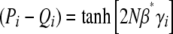, as if the ensemble were at a local stationary state under a selection gradient β*. Thus

(29)

It is easier to work in terms of β*. Multiplying by , we obtain a closed equation for β*:

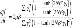(30)

When selection is weak , Equation 29 simplifies to 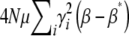. Since in this limit, this converges to . The exact solution, Equation 27, converges to the same limit with weak selection. This is as expected, since when selection is weak, the population approaches a mutation–drift equilibrium, with genetic variance ; the trait mean then changes at a rate due to selection and due to mutation.

Figure 10 shows an example where selection is strong, changing abruptly from Nβ = −4 to +4. The effects of 10 loci are drawn from a gamma distribution, as in Equation 25. The predictions for the mean are indistinguishable (Figure 10, left). There are substantial errors in the predictions for the underlying allele frequencies, with the rate of change of alleles of small effect being greatly overestimated (Figure 10, bottom curve at right) and that of alleles of large effect being slightly underestimated. However, these errors almost precisely cancel in their effects on the mean.

Figure 10.—

The maximum entropy approximation (Equation 29), made assuming that populations jump between fixed states, gives an accurate prediction for the change in mean (left): this is indistinguishable from the exact solution (Equation 27). The population is initially at equilibrium with directional selection Nβ = −4; selection then changes sign abruptly. Allelic effects are given by Equation 25. Predictions for the underlying allele frequencies are less accurate. (Right) Allele frequencies at the locus with the strongest effect , with intermediate effect , and with the weakest effect , reading left to right. Solid lines show the maximum entropy approximation (Equation 29), and dashed lines show the exact solution (Equation 27).

DISCUSSION

The maximum entropy approximation:

A fundamental aim of quantitative genetics is to understand the evolution of the phenotype, without knowing the underlying distribution of all possible gene combinations. Assuming linkage equilibrium simplifies the problem, which then depends only on the allele frequencies rather than on the full distribution of genotypes. However, if we include random drift, as well as selection and mutation, a full description of the stochastic dynamics requires the distribution of allele frequencies—a formidable task. We know that in general, we cannot predict phenotypic evolution without knowing the frequencies of all the relevant alleles: the future response to selection may depend on the frequencies of alleles that are currently so rare that they have negligible effect on the phenotype and so are essentially unpredictable. To avoid this difficulty, we make the key assumption that selection and mutation act only on observable quantities. Then, the distribution of allele frequencies tends toward a stationary state that depends only on those forces. If selection could instead act on individual alleles, it could send the population into arbitrary states by picking out particular alleles (e.g., Figure 1). Selection on individual alleles would be analogous to Maxwell's demon, which perturbs individual gas molecules to generate improbable states that violate the laws of classical thermodynamics (Leff and Rex 2003).

Populations tend toward a stationary state that maximizes entropy—that is, the distribution of allele frequencies spreads out as widely as possible, conditional on the average values of the quantities that are acted on by selection and mutation. The maximum entropy approximation to the dynamics amounts to assuming that the allele frequency distribution always maximizes entropy, given the current values of the observed variables, even though those variables may be changing. This approximation converges to the exact solution when changes in mutation and selection () are slow. However, we find that even if selection abruptly changes in direction, predictions for the trait mean are remarkably accurate.

The analogy between the population genetics of quantitative traits and statistical mechanics is intriguing. As well as suggesting methods for approximating phenotypic evolution, it also helps us to better understand the scope of statistical mechanics, by showing that it does not depend on physical principles such as conservation of energy (Ao 2008). Selection can be seen as generating information, by picking out the best-adapted genotypes from the vast number of possibilities, despite the randomizing effect of genetic drift. This is analogous to the way that a physical system does useful work, despite the tendency for entropy to increase. Such issues are discussed by N. H. Barton and J. B. Coe (unpublished data) and by H. P. de Vladar and I. Pen (unpublished data). Here, we concentrate on the use of maximum entropy as an approximation procedure.

Provided that the number of mutations, 4Nμ, is constant, and not too small, the method accurately predicts the evolution of the trait mean—even when allelic effects vary across loci, and even when selection changes abruptly. This accuracy even when parameters change rapidly is surprising, because the underlying allele frequencies may not be well predicted (e.g., Figure 10). Indeed, Prügel-Bennett, Rattray, and Shapiro make accurate predictions even though they use an arbitrary entropy measure that does not ensure convergence to the correct stationary distribution. Although we believe that our entropy measure is the most natural for quantitative genetic problems, and it does guarantee convergence to the stationary state, it may be that the maximum entropy approximation is an efficient method for reducing the dimensionality of a dynamical system, even when an unnatural measure is used.

The maximum entropy method predicts the full allele frequency distribution from just a few quantities, such as the expected trait mean, . We do still need to know the genetic basis of the trait—for an additive trait, we must know the allelic effects. We could hardly expect to predict the evolution of phenotype without knowing anything about its genetic basis. However, we could apply the method knowing just the distribution of allelic effects, which could be estimated in a number of ways: by detection of QTL, from evolutionary arguments about plausible distributions (e.g., Orr 2003), or from the distribution of allele frequencies at synonymous and nonsynonymous sites (e.g., Loewe et al. 2006).

Extension to dominance and epistasis:

We have analyzed only the simplest case, of directional selection on an additive trait. An extension to allow dominance is straightforward, since the loci still fluctuate independently of each other, and the generating function, , can still be written as a product of integrals across loci. Extension to more than two alleles is also possible, but only under the restrictive condition that mutation rates allow for detailed balance and hence for an explicit potential function. Similarly, alleles at different loci may interact in their effect on the trait. If such epistasis involves nonoverlapping pairs of loci, then calculations can still be made, but require integrals over pairs of allele frequencies. Although it is beyond the scope of this article to present such calculations, it is important to point out that, despite the technical difficulties, the method itself is general and as such it does not depend on the selective scheme, epistatic model, number of alleles, etc.

It is relatively straightforward to allow for stabilizing selection on an additive trait. In this case, allele frequency distributions at different loci are no longer independent. However, they are coupled only via a single variable, the trait mean: if this lies above the optimum, then all loci experience selection for lower , and vice versa. This simple coupling allows explicit solutions for the stationary distribution and for the rate of jumps between metastable states. These calculations are given in Barton (1989) and Coyne et al. (1997, Appendix). We outline the maximum entropy approximation to the dynamics of stabilizing selection in supplemental information D.

For complex models, involving epistasis between large numbers of genes, calculation of the maximum entropy approximation (i.e., of the matrices B*, C*) by numerical integration would not be feasible. They could still be calculated by a Monte Carlo method: one would fix the parameters and simulate the distribution to determine the expectations . The matrix C* could be found from the covariance of fluctuations, and the matrix B* from Equation 13. The two matrices, and , would then give the dynamics on the reduced space of this would be feasible numerically for two or three variables. Of course, this approach involves the same kind of computation as a direct simulation. Our claim is that the reduced dynamics will be approached, regardless of the initial allele frequency distribution: the system is expected to move close to the lower-dimensional space defined by the maximum entropy approximation. The implication is that we could predict the evolution of the expectations by a closed set of equations, without knowing the actual allele frequency distribution. This will require that we know the genetic basis and mutability of the trait and that selection acts only on that trait.

Low mutation rates (4Nμ < 1):

We describe mutation and selection by using a potential function , where 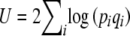, and include the variable together with selected variables such as the expectation of the trait mean, . However, this approach fails to describe the effects of changes in mutation rate when 4Nμ < 1, because then populations are likely to be close to fixation, in which case U diverges. The fundamental problem is that the distribution at the boundaries changes rapidly as mutation rate changes, while the bulk of the distribution does not. We can, however, extend the method to the case where 4Nμ is very small, because then populations jump between fixation for one or the other genotype, through the substitution of single mutations. This limit is in fact more general, in that it applies even with linkage or with asexual reproduction. It could be extended to give a more accurate approximation for appreciable 4Nμ, by calculating the probability of a jump between states of near fixation, taking into account the polymorphism at other loci (see Barton 1989).

Long-term response to selection:

A basic and long-standing puzzle in quantitative genetics is the success of artificial selection: in moderately large populations, traits respond steadily to selection for ≥100 generations, with little change in additive genetic variance and often with concordance between replicates (Barton and Keightley 2002). This is surprising, because the genetic variance is expected to change as alleles sweep through the population. However, if the distribution of allele frequencies is proportional to (pq)^4Nμ−1, as we assume, and if 4Nμ is small, then the additive genetic variance is expected to stay constant for long periods under directional selection. This is because the baseline distribution φ(p) = (pq)⁻¹ is uniform when transformed to a logit scale [i.e., φ(z) = constant for z = log(p/q)]. Since log(p/q) increases linearly with time under directional selection, that implies that the increase in genetic variance due to rare alleles increasing to become common is precisely balanced by the decrease due to common alleles approaching fixation. Thus, the response to standing variation is expected to continue steadily at a rate for ∼(1/s)log (2N) generations, whereas if alleles were typically polymorphic (as would be the case if 4Nμ > 1), it would continue for only ∼(1/s) generations. Of course, the response will continue indefinitely as a result of new mutation, at just the same rate. This is because variation is initially maintained in a balance between mutation and drift; the genetic variance is not affected by directional selection, and so the rate of response stays the same even as it shifts from alleles that were originally present to new mutations.

The stationary density under mutation, selection, and drift has been exploited before to help understand the evolution of quantitative traits (e.g., Keightley and Hill 1987; Keightley 1991). In this article, we have shown that the dynamics of polygenic traits can be accurately approximated by assuming that the underlying distribution of allele frequencies always takes this stationary form. We are now starting to get detailed estimates of the distribution of allele frequencies and of allelic effects on traits and on fitness (e.g., Loewe et al. 2006; Boyko et al. 2008): it may be that we will soon be able to use such data to apply the methods developed here to natural and artificial populations.

References

- Ao, P., 2008. Emerging of stochastic dynamical equalities and steady state thermodynamics from Darwinian dynamics. Commun. Theor. Phys. 49 1073–1090. [DOI] [PMC free article] [PubMed] [Google Scholar]
- Barton, N. H., 1986. The maintenance of polygenic variation through a balance between mutation and stabilizing selection. Genet. Res. 49 157–174. [DOI] [PubMed] [Google Scholar]
- Barton, N. H., 1989. The divergence of a polygenic system under stabilizing selection, mutation and drift. Genet. Res. 54 59–77. [DOI] [PubMed] [Google Scholar]
- Barton, N. H., and P. D. Keightley, 2002. Understanding quantitative genetic variation. Nat. Rev. Genet. 3 11–21. [DOI] [PubMed] [Google Scholar]
- Barton, N. H., and M. Turelli, 1987. Adaptive landscapes, genetic distance, and the evolution of quantitative characters. Genet. Res. 49 157–174. [DOI] [PubMed] [Google Scholar]
- Barton, N. H., and M. Turelli, 1989. Evolutionary quantitative genetics: How little do we know? Annu. Rev. Genet. 23 337–370. [DOI] [PubMed] [Google Scholar]
- Barton, N. H., and M. Turelli, 1991. Natural and sexual selection on many loci. Genetics 127 229–255. [DOI] [PMC free article] [PubMed] [Google Scholar]
- Boltzmann, L., 1872. Further studies on the thermal equilibrium of gas molecules. Sitzungsber. Akad. Wiss. Wien II 66 275–370. [Google Scholar]
- Boyko, A., S. Williamson, A. Indap and J. Degenhardt, 2008. Assessing the evolutionary impact of amino acid mutations in the human genome. PLoS Genet. 4 e1000083. [DOI] [PMC free article] [PubMed] [Google Scholar]
- Bürger, R., 1991. Moments, cumulants and polygenic dynamics. J. Math. Biol. 30 199–213. [DOI] [PubMed] [Google Scholar]
- Bürger, R., 1993. Predictions of the dynamics of a polygenic character under directional selection. J. Theor. Biol. 162 487–513. [DOI] [PubMed] [Google Scholar]
- Bürger, R., G. P. Wagner and F. Stettinger, 1989. How much heritable variation can be maintained in finite populations by mutation selection balance. Evolution 43 1748–1766. [DOI] [PubMed] [Google Scholar]
- Coyne, J. A., N. H. Barton and M. Turelli, 1997. A critique of Wright's shifting balance theory of evolution. Evolution 51 643–671. [DOI] [PubMed] [Google Scholar]
- Crow, J. F., and M. Kimura, 1970. An Introduction to Population Genetics Theory. Harper & Row, New York.
- De Groot, S. R., and P. Mazur, 1984. Non-Equilibrium Thermodynamics. Dover, New York.
- Ewens, W. J., 1979. Mathematical Population Genetics. Springer-Verlag, Berlin.
- Falconer, D. S., and T. F. C. Mackay, 1996. Introduction to Quantitative Genetics, Ed. 4. Longmans Green, Essex, UK.
- Gardiner, C., 2004. Handbook of Stochastic Methods. Springer-Verlag, Berlin.
- Georgii, H., 2003. Probabilistic aspects of entropy, pp. 37–56 in Entropy, edited by A. Greven. Princeton University Press, Princeton, NJ.
- Goldstein, S., and J. Lebowitz, 2004. On the (Boltzmann) entropy of non-equilibrium systems. Physica D 193 53–66. [Google Scholar]
- Gzyl, H., 1995. The maximum entropy method, pp. 27–40 in Series on Advances in Mathematics for Applied Sciences, Vol. 29. World Scientific, Singapore.
- Iwasa, Y., 1988. Free fitness that always increases in evolution. J. Theor. Biol. 135 265–281. [DOI] [PubMed] [Google Scholar]
- Keightley, P. D., 1991. Genetic variance and fixation probabilities at quantitative trait loci in mutation-selection balance. Genet. Res. 58 139–144. [Google Scholar]
- Keightley, P. D., and W. G. Hill, 1987. Directional selection and variation in finite populations. Genetics 117 573–582. [DOI] [PMC free article] [PubMed] [Google Scholar]
- Kimura, M., 1965. A stochastic model concerning the maintenance of genetic variability in quantitative characters. Proc. Natl. Acad. Sci. USA 54 731–736. [DOI] [PMC free article] [PubMed] [Google Scholar]
- Kirkpatrick, M., T. Johnson and N. Barton, 2002. General models of multilocus evolution. Genetics 161 1727–1750. [DOI] [PMC free article] [PubMed] [Google Scholar]
- Klein, G., and I. Prigogine, 1953. Sur la mecanique statistique des phenomenes irreversibles I. Physica 19 74–88. [Google Scholar]
- Lande, R., 1976. Natural selection and random genetic drift in phenotypic evolution. Evolution 30 314–334. [DOI] [PubMed] [Google Scholar]
- Le Bellac, M., F. Mortessagne and G. G. Batrouni, 2004. Equilibrium and Non-Equilibrium Statistical Thermodynamics. Cambridge University Press, Cambridge, UK.
- Leff, H. S., and A. F. Rex, 2003. Maxwell's Demon II. Institute of Physics, Bristol, UK.
- Lenormand, T., and S. Otto, 2000. The evolution of recombination in a heterogeneous environment. Genetics 156 423–438. [DOI] [PMC free article] [PubMed] [Google Scholar]
- Loewe, L., B. Charlesworth, C. Bartolome and V. Noel, 2006. Estimating selection on nonsynonymous mutations. Genetics 172 1079–1092. [DOI] [PMC free article] [PubMed] [Google Scholar]
- Nicolis, G., and I. Prigogine, 1977. Self Organization in Non-Equilibrium Systems: From Dissipative Structures to Order Through Fluctuations. John Wiley & Sons, New York.
- Onsager, L., 1931. Reciprocal relations in irreversible processes. I. Phys. Rev. 37 405–426. [Google Scholar]
- Orr, H. A., 2003. The distribution of fitness effects among beneficial mutations. Genetics 163 1519–1526. [DOI] [PMC free article] [PubMed] [Google Scholar]
- Prigogine, I., 1949. Le domaine de validité de la thermodynamique des phénomènes irréversibles. Physica 15 272–284. [Google Scholar]
- Prügel-Bennett, A., 1997. Modelling evolving populations. J. Theor. Biol. 185 81–95. [DOI] [PubMed] [Google Scholar]
- Prügel-Bennett, A., 2001. Modeling crossover-induced linkage in genetic algorithms. Evol. Comp. 5 376–387. [Google Scholar]
- Prügel-Bennett, A., and J. L. Shapiro, 1994. An analysis of genetic algorithms using statistical mechanics. Phys. Rev. Lett. 72 1305–1309. [DOI] [PubMed] [Google Scholar]
- Prügel-Bennett, A., and J. Shapiro, 1997. The dynamics of a genetic algorithm for simple random Ising systems. Physica D 104 75–114. [Google Scholar]
- Rattray, M., 1995. The dynamics of a genetic algorithm under stabilizing selection. Complex Syst. 9 213–234. [Google Scholar]
- Rattray, M., and J. Shapiro, 2001. Cumulant dynamics of a population under multiplicative selection, mutation, and drift. Theor. Popul. Biol. 60 17–32. [DOI] [PubMed] [Google Scholar]
- Renyi, A., 1961. On measures of entropy and information, pp. 547–561 in Proceedings of the Fourth Berkeley Symposium on Mathematics and Statistical Probabilities, Vol. 1. University of California Press, Berkeley, CA.
- Rogers, A., 2003. Phase transitions in sexual populations subject to stabilizing selection. Phys. Rev. Lett. 90 158103. [DOI] [PubMed] [Google Scholar]
- Rouzine, I., E. Brunet and C. Wilke, 2007. The traveling-wave approach to asexual evolution: Muller's ratchet and speed of adaptation. Theor. Popul. Biol. 73 24–46. [DOI] [PMC free article] [PubMed] [Google Scholar]
- Roze, D., and N. H. Barton, 2006. The Hill–Robertson effect and the evolution of recombination. Genetics 173 1793–1811. [DOI] [PMC free article] [PubMed] [Google Scholar]
- Sella, G., and A. E. Hirsh, 2005. The application of statistical physics to evolutionary biology. Proc. Natl. Acad. Sci. USA 102 9541–9546. [DOI] [PMC free article] [PubMed] [Google Scholar]
- Tsallis, C., 1988. Possible generalization of Boltzmann-Gibbs statistics. J. Stat. Phys. 52 479–487. [Google Scholar]
- Turelli, M., 1984. Heritable genetic variation via mutation-selection balance: Lerch's zeta meets the abdominal bristle. Theor. Popul. Biol. 25 138–193. [DOI] [PubMed] [Google Scholar]
- Turelli, M., and N. H. Barton, 1990. Dynamics of polygenic characters under selection. Theor. Popul. Biol. 38 1–57. [Google Scholar]
- Turelli, M., and N. H. Barton, 1994. Genetic and statistical-analyses of strong selection on polygenic traits: What, me normal? Genetics 138 913–941. [DOI] [PMC free article] [PubMed] [Google Scholar]
- van Kampen, N. G., 1957. Derivation of the phenomenological equations from the master equation. Physica 101 707–719. [Google Scholar]
- van Nimwegen, E., and J. Crutchfield, 2000. Optimizing epochal evolutionary search: population-size independent theory. Comp. Methods Appl. Mech. Eng. 9 171–194. [Google Scholar]
- Wehrl, A., 1978. General properties of entropy. Rev. Mod. Phys. 50 221–260. [Google Scholar]
- Wright, S., 1937. The distribution of gene frequencies in populations. Proc. Natl. Acad. Sci. USA 23 307–320. [DOI] [PMC free article] [PubMed] [Google Scholar]
- Wright, S., 1967. “Surfaces” of selective value. Proc. Natl. Acad. Sci. USA 58 165–172. [DOI] [PMC free article] [PubMed] [Google Scholar]