A systematic method for estimating individual responses to treatment with antipsychotics in CATIE

Abstract

Objective

In addition to comparing drug treatment groups, the wealth of genetic and clinical data collected in the Clinical Antipsychotic Trials of Intervention Effectiveness study offers tremendous opportunities to study individual differences in response to treatment with antipsychotics. A major challenge, however, is how to estimate the individual responses to treatments. For this purpose, we propose a systematic method that condenses all information collected during the trials in an optimal, empirical fashion.

Method

Our method comprises three steps. First, we test how to best model treatment effects over time. Next, we screen many covariates to select those that will further improve the precision of the individual treatment effect estimates which, for example, improves power to detect predictors of individual treatment response. Third, Best Linear Unbiased Predictors (BLUPs) of the random effects are used to estimate for each individual a treatment effect based on the model empirically indicated to best fit the data. We illustrate our method for the Positive and Negative Syndrome Scale (PANSS).

Results

A model assuming it takes on average about 30 days for a treatment to exert an effect that will then remain about the same for the rest of the trial showed the best fit to the data. Of all screened covariates, only two improved the precision of the individual treatment effect estimates. A comparison with more traditional post- minus pre-treatment symptom scores showed that our model based treatment effect estimates were a) more precise because they use all data collected during the trial rather than just two data points, and b) less sensitive to biases created by using the same baseline to calculate multiple treatment effects in CATIE.

Conclusions

We demonstrate that treatment effects can be estimated in a way that condenses all information collected in an optimal, empirical fashion. We expect the proposed method to be valuable for other clinical outcomes in CATIE and potentially other clinical trials.

1. Introduction

Schizophrenia is an often devastating neuropsychiatric illness (Sullivan, 2005) and effective pharmacotherapy is therefore critical from a mental health perspective. The Clinical Antipsychotic Trials of Intervention Effectiveness (CATIE, (Lieberman et al., 2005;Stroup et al., 2003) is an important resource for studying treatment with antipsychotics. As the use of atypical medications has steadily grown, one of the goals of CATIE was to examine whether these expensive medications can reduce morbidity and hospital use and improve community functioning, as compared to the conventional or first generation antipsychotic drugs.

Complications exist in that typically only a proportion of the patients suffering from schizophrenia respond to a specific antipsychotic (Kane, 1999). Misdosing, medication error, drug-drug interactions, and concomitant illnesses can sometimes provide an explanation. However, drug (non)-response may also reflect individual differences in disease etiology and biological variables that influence drug response. The several weeks it may take a clinician to declare a treatment ineffective and recommend an alternative may leave the schizophrenic patient vulnerable to continuing social dysfunction and suicide (Meltzer and Okayli, 1995) or possible side effects of the drug. Any improvement in our ability to match individual patients to the most effective and safe medication would therefore have substantial clinical benefits.

In addition to comparing treatments on a group level, many opportunities exist in CATIE to study individual differences in treatment response. Most notably, CATIE participants with DSM-IV schizophrenia and available DNA have now been genotyped for ~492,000 single nucleotide polymorphisms (SNPs, which are the most commonly used genetic markers) using the Affymetrix 500K genotyping platform plus a custom 164K chip to improve genome-wide coverage (Sullivan et al., 2008). This study therefore constitutes a tremendous resource for studying genetic modifiers of individual response to antipsychotics. This is particularly so because the genotype and clinical data are available to the scientific community from the controlled-access repository of the National Institutes of Mental Health (www.nimhgenetics.org).

The shift from comparing treatment groups to using the wealth of clinical and genetic data to better understand individual differences in responses presents novel methodological challenges. A major challenge here is how to best estimate individual responses to treatment with antipsychotics. In the case of CATIE this challenge is accentuated by the complex study design. For example, instead of a simple controlled randomized design with a drug and placebo group, CATIE was designed to evaluate the effectiveness of antipsychotic drugs in typical settings and populations so that study results will be maximally useful in routine clinical situations. Other salient features include the extensive data collection at multiple time points for a period up to 18 months. Furthermore, patients can be switched up to two times to a different drug for reasons such as lack of efficacy or drug toxicity.

In this article we propose a systematic method to estimate individual changes in clinically relevant outcomes during drug treatment in a way that condenses all information collected during the trial in an optimal, empirical fashion. Although such changes may not necessary be the (exclusive) result of the pharmacological action of the drug (e.g. there may be placebo effects, artifact due to repeated testing with same instrument etc), for sake of simplicity we will refer to these changes as estimates of the individual treatment effect.

Our model based approach has several potential advantages compared to more standard methods for estimating treatment effects (e.g., calculating post- minus pre-treatment symptom scores). First, using all, versus only a subset, of the assessments will improve the precision of the estimates and consequently the statistical power to detect correlates of the individual treatment effects. The latter is, for example, important in genomewide association studies (GWAS, where markers spanning the entire genome are tested for association with the outcome of interest) because genetic effects are likely to be small implying the need to maximize statistical power. Second, a wide variety of questions arise in complex trials such as CATIE including how to define treatment effects, how to handle the different treatment lengths, and what to do if only few observations are available. Our modeling approach provides a “natural” framework to address some of these issues. For example, there are multiple ways to define the treatment effect. Thus, instead of using the assessment obtained at the end of the treatment, for each patient we could also use the assessment after a predetermined period of treatment. The latter assessment will be more comparable across patients (e.g. in CATIE there is great variability in treatment duration), less confounded by the effects of being in the trial, and assuming that treatment effects will plateau will provide a good indication of the overall effect. However, rather than assume a priori which model of treatment response is more accurate, the method developed here enables empirical comparisons of various models and allows the selection of the treatment effect measure that is most consistent with the data. Finally, effects of potential confounders of treatment effects (e.g. changes as a result of repeated administration of the same diagnostic instrument) cannot be eliminated unless all data are considered. Such corrections may be important to further increase the precision of the treatment effect estimates.

Our method consists of first studying the best way to model treatment effects, then to screen many possible covariates to select those that will further improve the precision of the treatment effect estimates, and finally generate individual treatment effect estimates based on the best fitting model. We will demonstrate our method using the Positive and Negative Symptom Scale (PANSS, (Kay et al., 1987) that is a primary outcome in the CATIE study. In the final section we will study some of the properties of the estimated treatment effects and provide guidelines for subsequent analyses using these estimates. The method proposed in this article is generic and could potentially be valuable for other outcome variables in CATIE as well as other clinical trials.

2. METHODS

2.1 CATIE

A detailed description of the CATIE study can be found elsewhere (Lieberman et al., 2005;Stroup et al., 2003). In short, CATIE is a multiphase randomized controlled trial of antipsychotic medications where patients with DSM-IV schizophrenia were followed for up to 18 months. Preliminary diagnoses of schizophrenia were established by the referring psychiatrists and independently re-evaluated by CATIE personnel using the SCID (Structured Clinical Interview for DSM-IV, (First et al., 1994). The main exclusion criteria were a first episode of illness (because of diagnostic uncertainty) or being treatment-refractory (as alternative therapeutic approaches are indicated). To maximize representativeness, subjects were ascertained from clinical settings across the US (e.g., public mental health, academic, Veterans’ Affairs, and managed care centers). The mean age was 40.6 (SD=11.1) years. Seventy-four percent were male and racial composition was 60% white, 35% black, and 5% other. Eleven percent of the patients were married, and 85% unemployed. The mean number of years since an antipsychotic medication was first prescribed was 14.4 (SD=10.7).

Following provision of informed consent, a peripheral venous blood sample was obtained and sent to the Rutgers University Cell and DNA Repository (RUCDR) via overnight shipping where cell lines were established. DNA samples are currently available on 765 CATIE subjects. All these subjects have now been genotyped for ~492,000 single nucleotide polymorphisms (SNPs) using the Affymetrix 500K genotyping platform plus a custom 164K chip to improve genome-wide coverage (Sullivan et al., 2008). The genotype and clinical data are available to the scientific community from the controlled-access repository of the National Institutes of Mental Health (www.nimhgenetics.org). Current analyses will focus on the publicly available data set for which treatment effect estimates will be particularly useful in GWAS analyses.

PANSS

Extensive clinical data were collected in CATIE (Keefe et al., 2003). In this article we focus on the Positive and Negative Syndrome Scale (PANSS, (Kay et al., 1987) to illustrate our method for treatment effect estimation. The 30 items of the PANSS measure a broad range of the symptoms typical for schizophrenia. To unravel the structure of the PANSS items, a considerable number of factor analyses have been performed. Although variation exists, partly because of methodological differences (Van den Oord et al., 2006), a five factor structure is generally preferred (White et al., 1997). Because of their very large sample size (N = 5,769), we used the five scales derived by Van der Gaag et al. ((van der Gaag et al., 2006)see bold items in their Table 3) that are labeled Positive symptoms, Negative symptoms, Disorganization symptoms, Excitement, and Emotional distress along with the Total symptom score which is the sum of the 30 PANSS items.

Table 3.

Screening covariates for PANSS total symptom scores plus summary measures for other PANSS scales using LAG model c = 30 days as baseline

	Significance testing (df = 1)		% change compared to baseline model			Summary other scales
	Chi-sq.	P	Var(bik)	Var(ei)	Ratio	# p <.05	# Ratio > 1.01
Trial effects
In trial	134.9	0.000	0.680	0.998	0.681	6	0
Phase 1a	1.8	0.183	0.975	1.002	0.973	1	0
Phase 1b	13.4	0.000	0.984	0.998	0.986	5	0
Phase 2	3.9	0.048	0.984	1.000	0.984	3	1
Phase 3	71.8	0.000	0.980	0.983	0.997	6	0
Time in study (days)	306.7	0.000	0.631	0.966	0.654	6	0
Other study effects
End of phase	48.6	0.000	1.058	0.986	1.073	6	6
End of phase 1a	39.2	0.000	1.037	0.988	1.049	6	6
End of phase 1b	0.1	0.770	1.000	1.000	1.000	0	0
End of phase 2	27.4	0.000	1.020	0.993	1.028	5	5
End of phase 3	5.9	0.015	0.996	0.999	0.997	2	0
Follow up	30.6	0.000	1.003	0.992	1.011	5	4
Switched to other drug
Switched beginning	0.2	0.633	1.000	1.000	1.000	0	0
Inadequate response	119.5	0.000	1.058	0.976	1.084	6	6
Adverse effect	2.9	0.090	1.006	0.999	1.007	1	1
Demographic & clinical
Gender	2.6	0.108	1.000	1.000	1.000	3	0
Eur. American	2.1	0.146	1.000	1.000	1.000	3	0
Afr. American	1.4	0.236	1.000	1.000	1.000	2	0
Hispanic	10.3	0.001	1.000	1.000	1.000	5	0
Recent exacerbation	1.0	0.306	1.000	1.000	1.000	0	0
Years of education	4.5	0.034	0.999	1.000	0.999	4	0
Employment status	18.1	0.000	0.999	1.000	0.999	4	0
Years treated	4.0	0.045	1.000	1.000	1.001	2	0
Years 1st medication	3.5	0.063	1.000	1.000	1.000	1	0

Note. df is degrees of freedom, Chi-sq is the chi-square test statistics, Ratio equals Var(b_ik)/Var(e_i), # p < 0.05 is the number of PANSS scales for which the covariate had a significant effect using the chi-square statistic, and # Ratio > 1.01 is the number of PANSS scale for which the Ratio Var(b_ik)/Var(e_i) was larger than 1.01.

Drug treatment protocol

CATIE assessments began with a baseline assessment followed by Phase 1, a double-blinded randomized clinical trial comparing treatment with the second generation antipsychotics olanzapine, quetiapine, risperidone, or ziprasidone versus perphenazine (a midpotency first generation antipsychotic). If the initially assigned medication was discontinued, typically because of a lack of efficacy or adverse effects, the subject and clinician could choose between one of the following Phase 2 trials: (1) randomization to open-label clozapine or a double-blinded second generation drug that was available but not assigned in Phase 1; or (2) double-blinded randomization to ziprasidone or another second generation drug that was available but not assigned in phase 1. Phase 3 is for patients who discontinue the treatment assigned in phase 2 and involves an open-label treatment chosen collaboratively by the clinician and patient. The followup phase is for patients who are no longer willing to continue taking study medication or who have discontinued their phase 3 medication before 18 months from the time of initial randomization has elapsed. Followup phase participants are not provided with study medication but are followed naturalistically on their treatment of choice.

Table 1 shows the number of valid PANSS total symptom scores in each phase of the CATIE study. The total number of assessments for the 765 subjects on whom DNA was collected was 5,715 or a mean of 7.5 assessments per patient. Clearly, a more traditional approach that would define treatment using only 2 observations would not take optimal advantage of all available information.

Table 1.

Number of valid PANSS assessments for the 765 subjects in CATIE with DNA available

	Baseline	Phase 1a	Phase 1b	Phase 2	Phase 3	Follow-up	Total
During trial
Olanzapine		881	68	203	83		1235
Perphenazine		593	0	0	16		609
Quetiapine		655	99	125	68		947
Risperidone		786	59	188	68		1101
Ziprasidone		367	0	190	52		609
Clozapine			0	106	70		176
Other drug			0	0	167		167
Outside trial	764					107	871
Total	764	3282	226	812	524	107	5715

2.2 Statistical analyses

Overview

Our method comprises three steps. First, we study how to best model treatment effects. Second, we screen many possible covariates to select only those that further improve the precision of the treatment effect estimate. Third, we estimate the individual treatment effects based on the model that best fits the data and generates the most precise estimates.

For the analyses we used multilevel or mixed modeling (Goldstein, 1995;Searle et al., 1992). Instead of estimating the mean treatment effect for the sample as a whole (i.e., fixed effects constrained to be the same across subjects), mixed modeling essentially allows treatment effects to be different for individuals in the study (i.e., modeling random effects that are allowed to vary across subjects) by leveraging the fact that we have multiple assessments per patient during the trial. In the mixed model, the PANSS score y for subject i on the j^th occasion is:

$$y_{ij}=o_i+\sum _{k=1}^7{b}_{ik}{\mathit{DRUG}}_{\mathit{ijk}}+e_{ij}$$ (1)

where o is the intercept, b is the effect of the drug, DRUG is the drug, and e is the error and residual score. Intercept o is essentially an indicator of symptom severity. DRUG_ijk indicates the administration of drug k to subject i at occasion j. DRUG can be coded in various ways (see next section for details) and by comparing the fit to the data when using these different options we can empirically determine the most accurate specification for treatment effects. Finally, b_ik is perhaps the most critical term, in that it produces our estimates of individual differences in treatment response by allowing treatment effects to vary across subjects (hence it is subscripted i). In mixed modeling terminology, b_ik a random coefficient with variance VAR(b_ik).

We estimated the random effects of all the main CATIE drugs: olanzapine, perphenazine, quetiapine, risperidone, and ziprasidone. In addition, we estimated the random effect of clozapine that is only administered in phases 2 and 3 and combined all remaining drugs administered in Phase 3 into the category “Other drug”. Hence, in the summation term in (1) drug index k goes from 1 to 7 (= total number of drugs). Due to the small sample sizes, the Phase 3 drugs were not individually considered and lumped in the general category “Other drug”. This enabled us to keep the Phase 3 observations in the analysis, which may still be useful to improve the precision of, for example, the estimate of the intercept. The model was estimated assuming uncorrelated random effects to obtain a more stable solution and avoid optimization problems.

We used the R nlme package for model estimation. The maximum likelihood (ML) method of estimating the log-likelihood was used instead of the Restricted or Residual maximum likelihood (REML), which is the default. The reason was that ML estimation permits significance testing of both fixed and random effects. For nested models, model fit was compared using likelihood ratio tests (i.e., two times the difference between the log-likelihoods of two nested models is asymptotically chi-squared distributed with the difference in estimated parameters as the degrees of freedom).

Modeling treatment effects

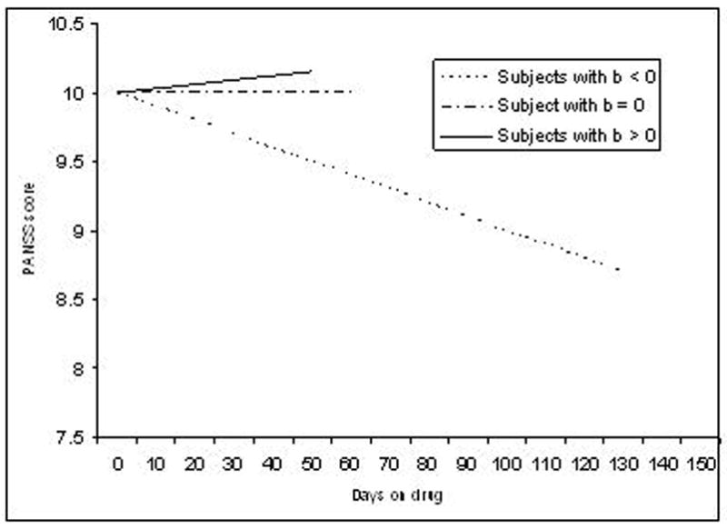
We considered two broad approaches to model treatment effects, each allowing variations. The first approach, labeled DOD (=days on drug), assumes that treatment effects continuously change as a function of the number of days a patient is on the drug. In the simplest case (Figure 1a), this change is linear where b_ik represents the change in PANSS per day for subject i when administered drug k. Thus, if b_ik < 0 then symptoms improve linearly (PANSS decreases), b_ik > 0 symptoms worsen linearly (PANSS increases), and if b_ik = 0 there is no treatment effect at all (PANSS remains the same). Note that if a subject is switched to another drug, then DRUG_ijk is reset to zero. Variations include adding a quadratic term (DRUG_ijk)2 to equation (1) to model possible curvilinear effects of the drug.

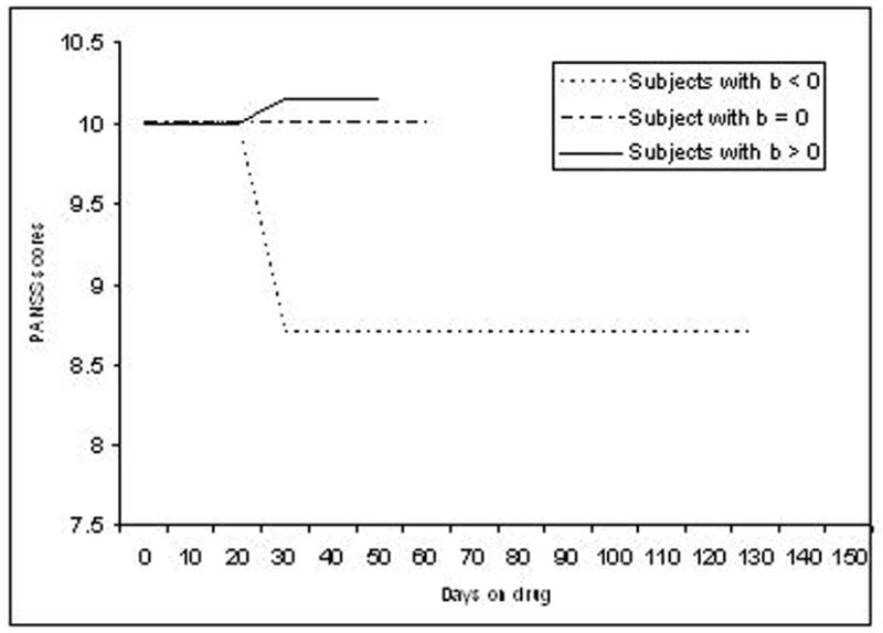
The second approach we considered assumes that if at the jth occasion subject i was on drug k less than c days then DRUG_ijk = 0 else DRUG_ijk = 1. This model (Figure 1b for c = 30) is labeled LAG as it assumes that will take c days for a drug to exert an effect (i.e., a “lagged” effect). Thus, if b_ik < 0 then symptoms improve after c days (PANSS decreases), b_ik > 0 symptoms worsen after c days (PANSS increases), and if b_ik = 0 there is no treatment effect at all (PANSS remains the same). If a subject is switched to another drug, then DRUG_ijk is reset to zero until c days on the drug elapse, after which the new drug indicator is then set equal to one as described above. Variations can be created by using different values for c.

Improving the quality of treatment effect estimates using covariates

Regressing out covariates could improve the precision of treatment effect estimates and consequently the statistical power to detect correlates of treatment effects. Roughly speaking, the precision of the treatment effect estimates is a function of the ratio of the treatment variance divided by the total variance that includes the treatment variance plus the error variance: VAR(b_ik)/(VAR(e_ij)+ VAR(b_ik)). More precise estimates will be obtained if the covariate reduces the error variance VAR(e_ij) and does not reduce the proportion of estimated treatment effect variance VAR(b_ik). The fact that reducing error improves the precision of the estimate follows directly from the ratio given above and seems self-explanatory. However, if that same covariate would reduce the treatment variance, then the ratio of the treatment variance divided by the total variance may actually become worse resulting in less precise treatment effects. Fortunately, in the mixed model we can estimate from the data how the covariate affects the treatment and error variances, and then based on those results decide which covariates to include.

To examine whether they could improve the precision of the treatment effect estimates we studied four groups of variables: 1) trial effects, 2) other study effects 3) the “Switched to other drug” group and 4) the demographic and clinical variables. Whereas covariates in the first three groups are time specific (e.g. “in trial” varies across time points in the trial), variables in the fourth group “Demographic and clinical variables” are subject specific (e.g. gender varies across subjects but remains the same across all time points during the trial). The “Trial effects” group contained candidates for capturing treatment effects other than those that are the result of drug treatment. Examples of such effects are changes in PANSS scores due to repeated testing with the same assessment instrument or personal interactions with clinicians. Effects of the variable “In trial” are non-zero if assessments during the trial differ from those at baseline and follow up. The other variables in this group (Phase 1a, Phase 1b, Phase 2, and Phase 3) account for phase specific effects. The final variable “Time in study” equaled the total number of days that a patient was in the CATIE study. It provides a more quantitative variable to capture the effect of being in the study. The “Other study effects” group includes the variable “End of phase” that allows each assessment made at the end of a phase to differ from the other assessments. Other variables in this group account for possible differences between the “End of phase” assessments of a specific phase (End of phase 1a, End of phase 1b, End of phase 2, and End of phase 3). “Follow up” captures differences between the follow up versus other assessments. The “Switched beginning” variable in the “Switched to other drug” group aims at capturing possible effects of being switched to a drug in Phase 1 that is different from the drug the patient took prior to being enrolled in the trial. The “Inadequate response” and “Adverse effect” variables indicate whether a patient was switched to another drug during the trial because the clinician thought the drug was not efficacious or produced adverse effects. Most labels of variables studied in the “Demographic and clinical” group (see Table 3) such as gender and employment status are self-explanatory. Exceptions are “Recent exacerbation” indicating whether a patient had been hospitalized or required crisis-stabilization services in the past three months for any mental health problem, “Years treated” indicating the number of years since patients was first treated for behavioral or emotional problem, and “Years since 1st antipsychotic” that is a count of the number of years since patients were first prescribed an antipsychotic medication.

Estimating individual treatment effects using BLUPs

After estimating the model parameters (means and variances) we can use these parameters to estimate the individual treatment effects by obtaining Best linear unbiased predictors (BLUPs) of the random effects (see supplementary material for technical details). The ability to condense all of the longitudinal treatment information into a single variable that represents the treatment effect is important from a practical perspective. For example, it will enable the “high-throughput” testing of hundreds of thousands of SNPs without fitting a full mixed model for every SNP, which will result in a massive reduction in computing time and avoid optimization problems that could occur (e.g., for SNPs with low minor allele frequencies).

3. Results

In this section we first determine how to best model the treatment effects. The two general models considered either assume that 1) treatment effect is a continuous function of time on a drug (DOD model in Figure 1a) or 2) treatment effect follows a step function where effects plateau after a fixed period of drug administration (LAG model in Figure 1b). The models will be compared in terms of how well they fit the data and the magnitude of correlations with a set of demographic and clinical variables. Next, we screen many possible covariates to select only those that further improve the precision of the treatment effect estimates. Finally, after estimating the individual treatment effects using the model that will generate the most precise estimates, we study the properties of the treatment effects in CATIE which may inform subsequent analyses of the data.

Modeling treatment effects

Because the DOD and LAG models have an equal number of parameters and are fitted on exactly the same data, the log-likelihood function values are directly comparable for a given scale (but not across scales) where less negative values indicate a better fit. In addition, for a given scale we can compare the residual variance VAR(e_ij) for the two models that will be smaller for the better fitting model. Adding a quadratic term (DRUG_ijk)2 to the DOD model to account for possible curvilinear effects of the drug did not substantially improve model fit. We therefore confined ourselves in Table 2 to the linear DOD model that only has DRUG_ijk as a predictor and is a more parsimonious model. In addition, we tested the LAG model with c = 0 (i.e., no lag effect), c = 30, and c = 60 days. The LAG model with c = 30 days gave the best fit to the data and we therefore only report these results in Table 2.

Table 2.

Fit indices from fitting linear DOD model and LAG model with c = 30

	Log Likelihood		Residual Variance
	DOD	LAG	DOD	LAG
Total symptoms	−91056	−90846	107.13	98.63
Positive symptoms	−61920	−61608	8.68	7.71
Negative symptoms	−68700	−68816	14.90	14.95
Disorganization symptoms	−56136	−56066	5.17	4.99
Excitement	−51676	−51388	3.86	3.52
Emotional distress	−56958	−56864	5.80	5.53

Comparing the fit of the linear DOD model and the LAG model with c = 30 days, Table 2 shows that the LAG model fitted consistently better than the DOD model with the exception of Negative symptoms. On average, the residual variances of the LAG model were about 7% smaller. This suggested a modestly better fit. Because a) the LAG model fitted better for the majority of scales and b) for negative symptoms the fit of the LAG and DOD model was are essentially equivocal, we proceeded with the LAG model.

Improving the quality of treatment effect estimates using covariates

Covariates were screened in Table 3 to examine whether they could improve the precision of the treatment effect estimates. Since the 30 day LAG model proved the best fit, covariates were added to this baseline model. The columns in Table 3 focus on the PANSS total. The columns under the heading “Significance testing” show that that the majority of the tested covariates are significantly correlated with one or more PANSS scales. However, in addition to reducing error variance, most covariates also reduce the variation in treatment effects. A conservative approach would be not to regress out these covariates as this may result in less precise treatment effect estimates and a subsequent reduction of statistical power to detect correlates of these treatment effects. For example, “Time in study” is significantly associated with PANSS total. However, in addition to reducing the residual variance to 96.6%, it reduced the variation in drug response VAR(b_ik) to 68.0%. Most likely, “Time in study” also captures part of the treatment effect. This could be because treatment effects are more likely to show later in the trial (e.g. takes some time for an effect to occur and patients are switched to another drug until there is some efficacy). Only the “End of phase” and “Inadequate response” variables have the desirable properties whereby they reduce the residual variance VAR(e_ij) and do not reduce the treatment effect variance VAR(b_ik). As a matter of fact they even improved the treatment effect variance a little. This could, for example, be because the clinical symptoms at the “End of phase” assessment are somewhat worse compared to other assessments during that phase (e.g. “End of phase” triggers a change to another drug, which could be related to a time specific drop in PANSS scores). The “End of phase 1a” and “End of phase 2” variables also showed smaller error variances and somewhat larger treatment effect variances. However, further significance testing showed that most of these effects were already captured by “End of phase” and little was gained by allowing the specific end of phase effects.

The analyses were repeated for all PANSS scales. Results, summarized in the final two columns of Table 3, were very similar. The column “# p < 0.05” in Table 3 shows that the majority of the tested covariates are significantly correlated with one or more PANSS scales. In addition, the column “# Ratio > 1.01” show that for all six other scales the “End of phase” and “Inadequate response” variables have the desirable property that they reduce the residual variance VAR(e_ij) and do not reduce the treatment effect variance VAR(b_ik)

Some properties of estimated treatment effects

We calculated correlations between estimated drug effects for PANSS total. We excluded clozapine and the “Other drug” category as the (pairwise) sample sizes were very small for these drugs. Table 4 shows that the resulting correlations tended to be small and negative. The exceptions seem to be some of the correlations involving Perphenazine but this could easily be the result of the small pairwise sample sizes. When we calculated similar correlations for the other drugs, we observed again that the correlations tended to be small and negative. Partly this could be caused by the CATIE design that switches patients to another drug when the first drug is not efficacious. Thus, it could still be that patients who respond to one drug would also have responded to another drug, resulting in a positive correlation, but this will not be observed in CATIE because these patients will remain on the efficacious drug. The implication is that simply combining treatment effects in CATIE across drugs may not result in an accurate measure of general drug effect.

Table 4.

Correlations (below diagonal) and pairwise sample sizes (above diagonal) among treatments effects for PANSS total

	Olanzapine	Perphenazine	Quetiapine	Risperidone	Ziprasidone
Olanzapine		25	61	59	49
Perphenazine	−0.192		28	22	11
Quetiapine	−0.192	0.398		58	44
Risperidone	−0.135	−0.254	0.066		53
Ziprasidone	−0.197	−0.895	−0.046	−0.345

It is important to realize that treatment effects are estimated as deviations from the intercept. Conceptually, the intercept is closely related to the mean of all observations during the trial after regressing out the drug effects. The use of the baseline observation would be problematic in this context as we would need to use the same baseline to calculate multiple treatment effects (e.g. subtract multiple “post-treatment” observations from the same baseline). The problem is that the baseline observation is affected by the true pre-treatment symptom score plus a random “measurement” error. If now, for example, the baseline PANSS score is low due to the random error, all estimated treatments effects for that patient will be underestimated because the same low baseline score is subtracted from each of the post-treatment scores. Because all treatment estimates will have a similar bias, they will be positively correlated in the whole sample. In the appendix, we show this phenomenon more formally and give a numerical example showing that it may easily cause substantial correlations even if the true treatment effects are uncorrelated.

In Table 5 we calculated correlations among PANSS scales for estimated olanzapine effects. Results show substantial positive correlations implying that drug effects tend to influence multiple symptom dimensions and are not restricted to specific symptom dimensions. Similar positive correlations were observed for the estimated treatment effects of the other drugs. These positive correlations seem to justify the use of the PANSS total symptom score as an outcome measure as that is an indicator of severity across the full range of symptoms.

Table 5.

Correlations (below diagonal) and pairwise sample sizes (above diagonal) among PANSS scales for estimated olanzapine effects

	Total symptoms	Positive symptoms	Negative symptoms	Disorganization	Excitement	Emotional distress
Total symptoms		254	254	254	254	254
Positive symptoms	0.725		254	254	254	254
Negative symptoms	0.785	0.351		254	254	254
Disorganization	0.723	0.480	0.498		254	254
Excitement	0.639	0.437	0.409	0.466		254
Emotional distress	0.634	0.370	0.348	0.247	0.337

4. Discussion

In this article we proposed a systematic method to estimate individual treatment effects for the PANSS that condensed all treatment information collected during the CATIE trial in an optimal, empirical fashion. This will facilitate the study of individual differences by, for example, enabling the “high-throughput” testing hundreds of thousands of genetic markers to detect the potential role of genetic variation.

A model assuming that it takes on average about 30 days for treatment to exert an effect that will then remain about the same for the rest of the trial showed the best fit to the data. Although we tested other models, this best fitting model is clearly a simplification of the complex and individual nature of treatment effects. In principle, more complex models can be fitted by adding further parameters. However, it may be important to note that this will also increase the complexity of any downstream analysis as each additional parameter will also result in an additional treatment effect measure. Thus, any improvement in fit should be large enough to justify the added complexity of having multiple effect estimates for a single drug.

The time course of antipsychotic treatment effects is a topic of considerable debate in the literature. Although the 30 day lag model in our study gave a better fit compared to the no lag and a 60 day lag model, the fact that in CATIE drug effects are not monitored on a daily basis limits the precision with which the lag can be determined. In this context it seems relevant to mention that a meta-analysis of the time course of antipsychotic response, incorporating 42 published studies and 7,450 patients, demonstrated the greatest response in the first 2 weeks, with a cumulative, though slowing improvement over time eventually expected to reach plateau (Agid et al., 2003). However, the authors focused on the first 4 weeks of treatment to show that significant improvements can be seen early on in treatment, and did not make definitive statements about the time of response plateau. A more recent met-analysis, this time incorporating 21 clinical trials and over 3,500 individuals, demonstrated a linear response pattern up to 28 days. This was followed by an attenuation, whereby the linear symptom reduction had plateaued by 6 weeks (Sherwood et al., 2006). Thus, based on existing literature, our 30 day assessment period would certainly capture the majority of expected symptom improvement.

Of all the covariates we screened, only two improved the precision of the treatment effect estimates. A general implication is that caution is warranted when regressing out the effects of covariates in studies where it is not possible to test whether this really improves treatment effect estimates. The risk is that the covariates may very well be associated with the treatment effects and by regressing them out we will obtain treatment effect estimates that are less precise and reduce the power to detect correlates of these treatment effects.

Two general recommendations can be made regarding further analyses of the CATIE PANSS data. First, we found that a given treatment tended to affect multiple symptom dimensions. This observation justifies the use of the PANSS total symptom score as an outcome measure as that is an indicator of severity across the full range of symptoms. Furthermore, in addition to searching for genes and other variables that affect drug response to specific symptom dimensions, it may therefore be meaningful to study how a given drug affects multiple symptom dimensions. Second, some caution seems warranted when trying to combine treatment effects in CATIE across drugs to create a generic treatment effect measure. Such a generic treatment effect measure may, for example, be desirable to study possible common mechanisms of antipsychotics. In CATIE, patients are generally kept on a drug that works and switched off a drug that they do not respond to. As a result, patients who have been treated with multiple drugs are those who do not respond to possible common mechanisms of action of the administered antipsychotics. This does not exclude the possibility that there may be groups of patients who do respond to multiple antipsychotics, it is just that the CATIE design makes it very difficult to discriminate between the variables that affect common versus specific drug pathways.

As with virtually any clinical trial, some subjects dropped out of the CATIE study. The subjects that left the study were not a random subset of the full sample, but were more likely to have higher symptom scores and poorer response to antipsychotic treatment. This raises the issue of how the missing data due to dropout influences the estimated treatment effects. If missingness is uncorrelated to the missing outcome value conditional on observed outcomes and model covariates, then missing data is considered missing at random (MAR) and estimates are unbiased and fully efficient, assuming the model is correctly specified (Rubin, 1976). Dropout in clinical trials is generally regarded as MAR if it can be shown that missingness is strongly predicted by observed outcome values {Cnaan, 1997 427/id}. Given that this is the case in the current analysis—individuals with high PANSS scores were more likely to dropout of the study—we suspect that missingness is largely MAR, though this is untestable given that the missing values are unknown. In the event that data is not MAR, or alternatively, if the missing observation follow a model other than the one specified, then the estimates would be biased, but the direction of the potential bias would be impossible to predict given that none of the relevant information is observed. It may, however, be pertinent to note that this article was not concerned with estimating the average treatment effect but estimating the individual treatment responses. If subjects with different treatment response patterns drop out, we speculate that a consequence may be reduced variance. This reduced variance could potentially result in, for example, diminished statistical power to detect correlates of the individual treatment effects.

The treatment effect estimates generated in this study are currently being used in a genome-wide association study (GWAS) to detect genetic modifiers of drug response. A major limitation of previous genetic studies is that they focus on a few markers in (candidate) genes hypothesized to be relevant as potential modifiers of drug response. The problem, however, is that current knowledge about the underlying mechanisms of drug action is limited so that it has been very difficult to find the genes that modify response to antipsychotics. GWAS offers the possibility of systematically screening genetic markers across the whole genome for association with drug response without relying on prior biological information. It is now clear that GWAS can be a successful strategy, as there have been multiple successes with the identification of highly compelling candidate genes for age-related macular degeneration (Klein et al., 2005), body mass index (Frayling et al., 2007), inflammatory bowel disease (Duerr et al., 2006) and type 2 diabetes mellitus (Saxena et al., 2007;Scott et al., 2007;Steinthorsdottir et al., 2007). GWAS findings could eventually facilitate tailoring the prescription of existing drugs to individual patients based upon genotype. Matching patients to the most effective and safe medication would have substantial clinical benefits. For example, delays in prescribing the most effective treatment may leave the patient vulnerable to continuing dysfunction and ineffective drugs may put the patient at an unnecessary risk for adverse events. Genetic markers would potentially have a number of advantages for tailoring pharmacotherapy such as being cost-efficient, prognostic, and can be measured in biomaterial (blood, saliva) that is easy to collect.

In addition to being useful for (other outcomes in) CATIE, the proposed method could be valuable for other clinical trails in particular those that have complex designs. That is, our method handles complexities such as multiple treatments, variable treatment lengths, drop out, and the choice of a “baseline” for multiple treatments in a natural way. Furthermore, it offers tools to evaluate different definitions of treatment effects and select covariates in an empirical way. Similar to traditional post- minus pretest scores, the estimated treatment effects are simple variables that can be used in follow up analyses without the need for complex statistical approaches. However, because our estimated treatment effects condense all information collected during the trials in an optimal and empirical fashion, they are potentially more precise and powerful to study determinants of treatment outcomes.