A Model Coupling Vibrational and Rotational Motion for the DNA Molecule

Abstract

We investigate a mechanical model for the DNA molecule using an extension of the Peyrard and Bishop model. In the present model, there are two chains of oscillators linked by a Morse potential, which represent the hydrogen bonds. The rotational and vibrational motions of each base pair are considered and the coupling for these motions are introduced by a nonlinear combination of them in the Morse potential. In this context, thermodynamics and structural properties are discussed.

Introduction

DNA is one of the most important macromolecules for life. Since the discovery of its structural form [1], several aspects of the DNA molecule have still not been unmasked. Theoretical studies of the functional mechanisms of this macromolecule involve the study of the interaction energies of DNA base pairs using a quantum mechanical formalism [2], the influence of topological changes on the potential energy for the phase transition [3], nonlinear dynamics [4, 5], and thermodynamic models (as, for example, the Poland–Scheraga model [6, 7]). The studies concerning nonlinear dynamics [8] were stimulated by the treatment of nonlinear waves and their possible role in the regulation of the biological processes. The possibility that the vibrational energy in the DNA could be dealt with using a model of the excitement of solitary waves was suggested two decades ago [9]. Recently, single-molecule experiments have contributed in to clarifying important dynamical aspects of this macromolecule, as, for example, DNA bubbles [10–12] and DNA intercalation [13].

A largely used mechanical model for vibrational motion of DNA has been proposed by Peyrard and Bishop (PB) [5]. In this model, DNA is represented by a pair of harmonic chains coupled by a nonlinear potential. The most frequently used nonlinear potential for this purpose is the Morse potential [14–17]. Some extensions of the original model in [5] are proposed considering, for example, the helicoidal structure of DNA [18]. An important objective for this kind of model is to understand the phenomenon of thermal denaturation and, through this, get some knowledge about other processes such as the genetic transcription and drug intercalation. It is possible to obtain from this type of model interesting properties, such as the average stretching between base pairs as a function of the temperature using the transfer integral operator [19]. Dynamical properties of this model were also explored and several phenomenological quantities are studied, such as energy localization, as in [20].

In this work, we extend the original PB model [5] by introducing rotational motions for the nucleotides. In this way, both the vibrational and rotational motion for each nucleotide are considered. The stretch of the base pairs is given by the Morse potential in the same way as in the original PB model. However, the coupling between the two kinds of motion, rotation and vibration, is obtained through a nonlinear combination of them in the Morse potential.

The Model

The original PB model to treat the statistics and dynamics of DNA works only the vibrational motions corresponding to the displacements from the equilibrium position of the hydrogen bonds. In the present work, we include rotational motion in the model and couple it with vibrational motion. Each nucleotide is represented by a disc of mass m and radius r. These discs are joined along the ribbon by spring potentials with coupling constants of strength k. The two ribbons are coupled by a nonlinear potential V_j, simulating the hydrogen bonds. For simplicity, we restrict ourselves to rotations of the discs around axis parallel to the helical axis, assumed perpendicular to the H-bond plane: while the linear displacements occur in this plane. Then, the movement of the disc is composed of two displacements: the linear, denoted by u_j (or v_j for the disc in the other ribbon) and the angular, denoted by θ_j (or ϕ_j at the complementary ribbon). Note that θ_j and ϕ_j are positive when the rotation is counter-clockwise, although the reference is different for each one (see Fig. 2). In this way, the V_j potential coupling the base pair is a function V(u_j,v_j,θ_j,ϕ_j). Figure 1 shows a representation of the model.

Fig. 2.

Displacement x of the disc j

Fig. 1.

Mechanical model consisting of two connected chains of mass-spring oscillators

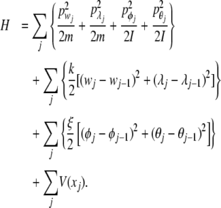
The Hamiltonian for the system can be written as

1

where

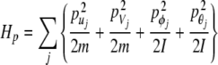2

represents the kinetics energy of the system, and

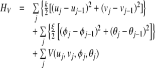3

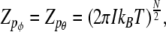
is the potential energy. In (2), and are the linear moments and and are angular moments. For simplicity, the system is considered homogenous, which means that the mass m and the moment of inertia I are equal for all nucleotides. For the same reason, the strength constants k and the angular strength constants ξ are the same for the entire system. Figure 1 shows a representation of the mechanical model indicated by (1).

The displacement of the H bond between two adjacent discs j is represented in Fig. 2 and can be written as

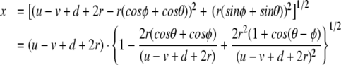4

where r is the radius of the discs and d is the equilibrium distance between them. Observing that r/(u − v + d + 2r) < 1 is always true, we can expand (4), as a function of this parameter, and the result up to the second order in r/(u − v + d + 2r) is:

We note that, to a first-order approximation, the angular variables already contribute to the displacement. In this approximation, the total displacement x is given by

5

Using this approximation in the Hamiltonian function (1) and changing the coordinates u_j and v_j by

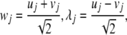6

we obtain the final form for the Hamiltonian:

7

The interaction between two adjacent bases is given by the Morse potential [5], i.e.,

8

where D is the energy of dissociation of the base pair, a is a parameter with dimension of inverse length, x₀ = 2r + d is the equilibrium point (the distance between the centers of the discs), x is given by (5), and the function g(ϕ,θ) is given by

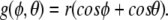9

It is important to remember that the potential V(x) is applied to vibrational motion, and the masses undergoing vibrational motion are assumed to be points. However, a correction on the displacement x dues by the rotation motion of the disc have been introduced by the adding of the angular terms as showed in (5). The Morse potential, (8), is generally chosen to simulate hydrogen bonds in DNA molecules (see, for example, [14–17]).

For a chain with N pairs of bases, the classic partition function is given in terms of the Hamiltonian (7) and can be factored as

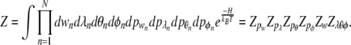10

The integrals in all moments are simple Gaussian integrals and give

11

and

12

where k_B is the Boltzmann constant.

The Z_w corresponds to contribution from the harmonic chain of oscillators. It is an easy task to calculate this integral, which involves Gaussian integrals, and the result is given by

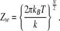13

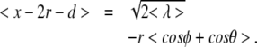
The integrals evaluated in order to obtain Z_w is similar to the harmonic part of the integration in [5]. Then, in order to study the average displacement < x − 2r − d >, only the interaction involving the coordinates λ, ϕ, and θ will be considered, i.e., we will study the function

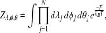14

where F is given by

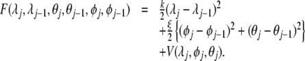15

The integral over λ in (14) can be calculated using the eigenfunctions and eigenvalues of a transfer integral operator [19]

16

The terms dependent on ϕ and θ are fixed when the integration over λ is performed. In the thermodynamic limit , the partition function Z_λ reduces to

17

where ε₀ is the ground state eigenvalue for a Schrödinger-like equation given by [5]:

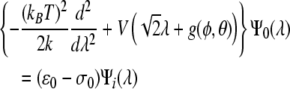18

where

19

The eigenvalue and the normalized eigenfunction for the ground state of (18) are, respectively,

20

and

21

where and C is the normalization constant. In the limit , the average stretching < λ > will be dependent only on the ground state eigenfunction as

22

< λ > (θ,ϕ) has a dependence on angles ϕ and θ, thus it is necessary to do an addition average over these coordinates in order to calculate the mean stretching obtained by (5):

23

where is an average of (22) over the angles θ and ϕ. The calculation of will be discussed in the following sections.

Results

The values of the parameters used are in the range of values presented in the literature and are based on experimental results as, for example, the scattering of neutrons [8] and experiments with single-molecule [16] and low-frequency vibrational modes [17]. From [16], as suggested, we get an upper bound for the combination of Morse parameters D and a, i.e., Da/2 ≤ 75 pN, and from [8], we get ξ = 2.0 eV. The value of r is obtained calculating the average radius of gyration for the four types of nucleotides using PDB data (www.rcsb.org). The adopted value here is r = 4Å.

Following the above criteria, we obtain an optimal set of parameters as: ξ = 2.0 eV, r = 4 Å, k = 0.06 eV Å^− 2, a = 2.81Å^− 1, and D = 0.03 eV. From these values, we note that Da/2 ≈ 67 pN ≤ 75 pN [16]. Using this set of parameters, the model becomes completely defined.

In order to analyze the results of the model, let us first explore two extreme situations on ϕ and θ. The average value of λ depends on θ and ϕ through (21) and (22) with g(θ,ϕ) given by (9). However, g(θ,ϕ) is a function bounded by θ and ϕ varying between − π/2 and π/2. At these limits, the hydrogen bonds are broken. Then, 0 ≤ g(θ,ϕ) ≤ 2r. For the extreme values of g(θ,ϕ), i.e., g(θ,ϕ) = 0 and g(θ,ϕ) = 2r = 8 Å, we can integrate numerically (22), and we get the average stretching of the bonds as a function of temperature. This is shown in Fig. 3 by the continuous and the triangle-symbol curves. In these cases, the angle dependence disappears and the average stretching is adopted to be < λ > as usual [5, 12]. Both curves indicate the same denaturation temperature; however, they have a quite different behavior for low temperatures.

Fig. 3.

Variation of the average stretching as a function of temperature, for three different contributions of g(θ,ϕ): zero (solid line) and 8.0 (triangles). The intermediate points (boxes) are obtained by integration of the complete expression for g(θ,ϕ) and admitting < θ > = < ϕ > = α

A more complex calculation is needed for estimating the dependence of the average stretching of θ and ϕ. Here, we restrict ourselves to the situation where the mean values of θ and ϕ are equal, i.e., < ϕ > = < θ > = α, and (9) becomes g(α) = 2rcosα with − π/2 < α < π/2. In this case, the average stretching of H-bonds indicated by (23) becomes

24

The final average for each temperature is obtained using the partition function (14), assuming θ = ϕ = α:

25

where < λ > (α) is given by (22) and is obtained from (14). We observe, from (20), that ε₀ has no angular dependence and its contribution to (25) cancels out. This happens because of the particular dependence of Morse potential on the angular variables due to the approximation in (5). In the adopted approach, the integration of (22) gives, as a general result, a function dependent on the angle α for each temperature. In the numerical calculation, the difference Δα_j is considered constant (Δα = 0.01) and the integration over α_j is done in discrete steps. The same procedure is used to determine the value of < cosα >. In order to check the accuracy of the calculation, an additional calculation through Monte Carlo methods was performed to determine the mean value < cosα >. The results are quite similar to the values obtained by the procedure proposed here.

The points (boxes) in Fig. 3 show the values obtained for < x − 2r − d > as function of temperatures and varying α in the interval [ − π/2,π/2]. We observe that the three curves presented in Fig. 3 diverge close to 350 K, which is adopted as the melting temperature. The denaturation temperature obtained is compatible with the experimental results observed, for example, using absorbance UV light at 260 nm [21].

Conclusion

The model introduced predicts realistic values for the melting temperature when acceptable parameters are used, in particular, k = 0.06 eV Å^− 2, ξ = 2.0 eV, a = 2.81Å^− 1, D = 0.03 eV, and r = 4Å. The introduction of rotational and vibrational motion in the same mathematical model contributes to a closer description of the real DNA.

The results (Fig. 3) indicate that the vibrational motion is the main contribution to DNA denaturation. However, the gap between the curves at low temperature is due to changes in the angular coordinates. Then, the rotation can be important for low-temperature effects such as, for instance, the “transcription bubble,” which moves along the DNA and tends to grow at high temperature [21]. Therefore, rotational and vibrational motion could have different roles in the DNA.

The accuracy of the model can be improved by considering a higher-order approximation in r/(u − v + d + 2r) in (4). In this case, it is necessary to improve the mathematical tools in order to obtain numerical results. Furthermore, the dynamical aspects of the proposed model can introduce important properties related to rotational motion of the base pairs of DNA, which cannot be observed by a simple vibrational model. Finally, we observe that, if the angular contribution is ignored, i.e, if g(θ,ϕ) = 0, we recover the original Peyrard–Bishop model.

References

- 1.Watson, J.D., Crick, F.H.C.: Molecular structure of nucleic acids. Nature 171, 737–738 (1953) [DOI] [PubMed]
- 2.Danilov, V.I., Kudritskaya, Z.G.: Quantum mechanical study of bases interactions in various associates in atomic dipole approximation. J. Theor. Biol. 59, 303–318 (1976) [DOI] [PubMed]
- 3.Grinza, P., Mossa, A.: Topological origin of the phase transition in a model of DNA denaturation. Phys. Rev. Lett. 92(15), 158102(1–3) (2004) [DOI] [PubMed]
- 4.Yakushevich, L.V.: Nonlinear DNA dynamics: a new model. Phys. Lett. A 136(7), 413–417 (1989) [DOI]
- 5.Peyrard, M., Bishop, A.R.: Statistical mechanics of a nonlinear model for DNA denaturation. Phys. Rev. Lett. 62(23), 2755–2758 (1989) [DOI] [PubMed]
- 6.Poland, D., Scheraga, H.A.: Theory of Helix-Coil Transitions in Biopolymers. Academic Press, New York (1970)
- 7.Wartell, R. M, Benight, A.S.: Thermal denaturation of DNA molecules: a comparison of theory with experiment. Phys. Rep. 126, 67–107 (1985) [DOI]
- 8.Fedyanin, V.K., Yakushevich, L.V.: Scattering of neutrons and light by DNA solitons. Stud. Biophys. 103, 171–178 (1984)
- 9.Englander, S.W., Kallenbach, N.R., Heeger, A.J., Krumhansl, J.A., Litwin, S.: Nature of the open state in long polynucleotide double helices: possibility of soliton excitations. Proc. Natl. Acad. Sci. U. S. A. 77, 7222–7226 (1980) [DOI] [PMC free article] [PubMed]
- 10.Ambjörnsson, T., Banik, S.K., Krichevsky, O., Metzler, R.: Sequence sensitivity of breathing dynamics in heteropolymer DNA. Phys. Rev. Lett. 97, 128105 (2006) [DOI] [PubMed]
- 11.Ambjörnsson, T., Banik, S.K., Krichevsky, O., Metzler, R.: Breathing dynamics in heteropolymer DNA. Biophys. J. 92, 2674 (2007) [DOI] [PMC free article] [PubMed]
- 12.Altan-Bonnet, G., Libchaber, A., Krichevsky, O.: Bubble dynamics in double-stranded DNA. Phys. Rev. Lett. 90, 138101 (2003) [DOI] [PubMed]
- 13.Vladescu, I.D., McCauley, M.J., Rouzina, I., Williams, M.C.: Mapping the phase diagram of single DNA molecule force-induced melting in the presence of ethidium. Phys. Rev. Lett. 95, 158102 (2005) [DOI] [PubMed]
- 14.Gao, Y., Prohofsky, E.W.: A modified self-consistent phonon theory of hydrogen bond melting. J. Chem. Phys. 80, 2242 (1984) [DOI]
- 15.Gao, Y., Devi-Prosad, K.V., Prohofsky, E.W.: A self-consistent microscopic theory of hydrogen bond melting with application to poly (dG)-poly(dC). J. Chem. Phys. 80, 6291–6298 (1984) [DOI]
- 16.Zdravković, S., Satarić, M.V.: Single-molecule unzippering experiments on DNA and Peyrard–Bishop–Dauxois model. Phys. Rev. E 73, 021905(1–11) (2006) [DOI] [PubMed]
- 17.Drigo Filho, E., Ruggiero, J.R.: Parameters describing the H bond in DNA. Phys. Rev. A 44(12), 43–44 (1991) [DOI] [PubMed]
- 18.Zdravkovic, S., Satarić, M., Tuszyński, J.: Biophysical implications of the Peyrard–Bishop–Dauxois model of DNA dynamics. J. Theor. Comput. Nanosci. 1, 171–181 (2004)
- 19.Scalapino, D.J., Sears, M., Ferrell, R.A.: Statistical mechanics of one-dimensional Ginzburg–Landau fields. Phys. Rev. B 6, 3409–3416 (1972) [DOI]
- 20.De Luca, J., Drigo Filho, E., Ponno, A., Ruggiero, J.R.: Energy localization in the Peyrard–Bishop DNA model. Phys. Rev. E 70, 026213(1–9) (2004) [DOI] [PubMed]
- 21.Peyrard, M.: Nonlinear dynamics and statistical physics of DNA. Nonlinearity 17, r1–r40 (2004) [DOI]