

Abstract
This protocol details the steps used for visualizing the frozen-hydrated grids as prepared following the accompanying protocol entitled ‘Preparation of macromolecular complexes for visualization using cryo-electron microscopy.’ This protocol describes how to transfer the grid to the microscope using a standard cryo-transfer holder or, alternatively, using a cryo-cartridge loading system, and how to collect low-dose data using an FEI Tecnai transmission electron microscope. This protocol also summarizes and compares the various options that are available in data collection for three-dimensional (3D) single-particle reconstruction. These options include microscope settings, choice of detectors and data collection strategies both in situations where a 3D reference is available and in the absence of such a reference (random-conical and common lines).
INTRODUCTION
Cryo-electron microscopy (cryo-EM) has gained popularity in structural biology because it enables visualization of macromolecular complexes in three dimensions in functionally relevant states. Several manufacturers produce electron microscopes that are well suited for visualizing frozen-hydrated samples using low-dose methods, the most often used being cryo-transmission electron microscopes (TEMs) made by FEI and JEOL. Based on the specific experience in our laboratory, this protocol details the steps used while employing FEI Tecnai TEMs. Further details concerning the advantages as well as the limitations of the cryo-EM technique can be found in the accompanying protocol by Grassucci et al.1. This protocol discusses the steps that follow grid preparation. The microscope imaging conditions and data collection schemes that will best answer the scientific question for a specific project while at the same time minimizing the level of beam damage to the biological sample (low-dose imaging) are discussed here. This protocol addresses the choices of several options available, such as pixel size, magnification, recording medium, accelerating voltage and defocus range (a comprehensive description of these options, along with a detailed description of reconstruction techniques, can be found in refs. 2-4). This is the standard protocol used in this laboratory. For instance, it has been employed to investigate the interaction of the hepatitis C virus’s internal ribosome entry site with the host’s translation machinery5, the tRNA selection process during decoding6 and the interaction of the signal recognition particle with the elongation-arrested ribosome7. An outline of the necessary steps is given in Figure 1.
Figure 1.
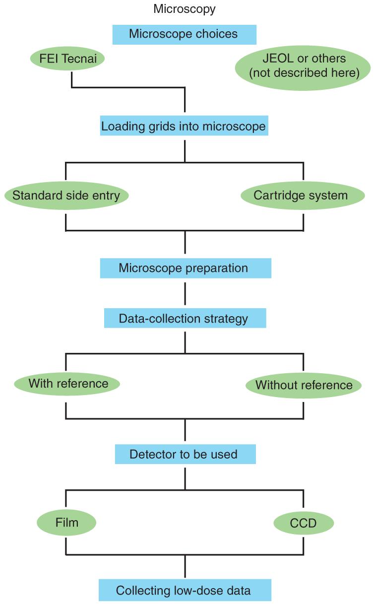
Schematic representation of steps in cryo-EM.
The majority of cryo-EM data are collected with FEI or JEOL microscopes. Although the general procedure for aligning the electron beam and acquiring data is similar for both systems, there are differences in the detailed steps. This protocol is tailored for the use of FEI Tecnai microscopes.
MATERIALS
EQUIPMENT
-
·
Kodak SO163 electron image film
-
·
Kodak D19 developer
-
·
Kodak rapid fixer
-
·
Buffer computer with greater than 2 TB of storage capacity
-
·
Cryo-TEM such as Tecnai F20 (with cryo-box) or Tecnai F30 Polara(http://www.fei.com/)
-
·
Cryo-transfer holders such as Gatan CT3500 cryo-transfer holder, Gatan 626 cryo-transfer holder (http://www.gatan.com/holders/) or FEI cartridge system available on F30 Polara (http://www.fei.com/)
-
·
CCD camera such as TVIPS TemCam F415 (http://www.tvips.com/), Gatan 795 CCD camera (http://www.gatan.com/imaging/) or FEI Eagle CCD camera (http://www.fei.com/)
PROCEDURE
Transfer of frozen grid to microscope ● TIMING 30 min
1| Select the cryo-transfer system you will be using (the type of sample stage is dependent on the microscope that will be used. See Step 25 of the accompanying protocol by Grassucci et al.1 for a description of handling precautions). To ensure optimal performance, the cryo-transfer holders are periodically pumped down with a dry pumping station. Option A describes the use of standard side-entry cryo-transfer holders and option B describes the procedure for using the cryocartridge system available on FEI Polara microscopes.
- Side-entry cryo-transfer holder
- To load the frozen-hydrated grid into the cryo-transfer holder, remove a well-evacuated cryo-transfer holder from the pumping station after ensuring that all the valves on the holder and the station are closed.
- Place the holder, the transfer station and the temperature controller on the bench adjacent to the microscope (see Fig. 2).
- Place a clip ring on the clip-ring tool.
- Insert the cryo-transfer holder into the workstation. Fill the workstation and dewar of the cryo-transfer holder with liquid nitrogen. Put the cover on the workstation.
- Wait for liquid nitrogen to ‘boil over’ and then refill the dewar and workstation so that the tip of the cryo-transfer holder is kept cold. Maintaining a positive pressure in the workstation, that is, a flow of vapor out of the workstation, will minimize the amount of contamination introduced. See Figure 2 of accompanying protocol by Grassucci et al.1 for examples of contamination.
- Plug the temperature controller into the cryo-transfer holder and wait until the tip achieves its minimum temperature (∼ -194 °C).
- With pre-cooled large tweezers, transfer the cryo-grid box from a small dewar to the workstation (see Fig. 3).
- Precool the tweezers and the clip-ring tool by placing them into the liquid nitrogen in the workstation.
- Remove the grid from the grid box using the precooled tweezers and place it into the sample-holder cup with the sample side facing upward.
- Quickly press the clip ring into position (or screw it into a cryo-cup with screw ring). Release the clip ring from the tool.
- Quickly close the cryo-shutter and remove the tools from the workstation.
- Refill the workstation with liquid nitrogen and remove the grid box from the workstation.
- Bring the workstation to the microscope and begin the pre-pump airlock cycle on the microscope via the Tecnai vacuum GUI.
- Wait for the airlock to be properly pre-pumped (120 s) as indicated by the red light on the stage being extinguished.
-
Set the stage position to X = 0 and Y = 0.▲ CRITICAL STEP Tilt the stage to -65 ° to prevent emptying of the cryo-transfer dewar during loading.
-
Carefully remove the cryo-transfer holder from the transfer station and insert it into the compu-stage.▲ CRITICAL STEP The guide pin on the cryo-transfer stage will be at 12 o’clock and must be quickly rotated clockwise to approximately 3 o’clock so that it engages the mating groove in the airlock. When the position is correct, the holder will slide into the airlock 2 cm further.
- Wait for the airlock pumping cycle to finish (120 s) as indicated by the red light on the compu-stage being extinguished.
- Rotate the cryo-holder so that the top is at 12 o’clock.
- Reset the tilt to 0 ° using the stage GUI.
- Refill the dewar on the cryo-holder.
- When the column vacuum level has reached the pre-loading level, the sample is ready to be viewed.
- Cartridge-loading system (available on FEI Polara)
- Precool the insertion rod and multispecimen chamber (MSC) while they are attached to the microscope. This will take approximately 30 min. Approximately 8 liters of liquid nitrogen will be needed for the following procedure.
- Cool the adsorption pump on the transfer station using approximately 5 liters of liquid nitrogen.
- Remove the cover from the cartridge-loading area and place the empty cartridges that will be loaded into their loading positions. Cool the cartridge-loading area with liquid nitrogen (see Fig. 4).
- When the liquid nitrogen boils over, replace the cover and fill the chamber with liquid nitrogen. The temperature in the loading area will now be below the devitrification temperature and frozen-hydrated samples can be safely transferred.
- Retrieve the frozen-hydrated sample from storage and place the grid box into the precooled loading vessel.
- Pick up the frozen-hydrated grid with precooled tweezers and place it with the sample side upward into the cartridge.
- Precool the c-clip tool and place it into the depression in the cartridge.
- Depress the plunger on the tool to slide the ring into place in the cartridge. The grid should now be anchored by the c-ring.
- Visually inspect the cartridge to ensure that the grid is properly mounted. An illuminated magnification device is helpful for this.
- Repeat Steps (vii-x) to load other samples if necessary. A total of six cartridges can be loaded into the chamber at one time.
-
Make a list of samples and their corresponding positions in the MSC. Make a note of which cartridge is loaded in the column.▲ CRITICAL STEP An empty space must be left in the MSC for any cartridge currently loaded in the column.
- Return the unused grids in the grid box to a liquid nitrogen storage dewar.
- Remove the precooled MSC from the microscope using the correct venting procedure. Click the ‘vent airlock’ button and follow the subsequent prompts given by the Tecnai vacuum user interface (UI).
- Mount the MSC on the transfer station (see Fig. 6).
- Turn on the diaphragm pump.
- Open valve 3 (roughing) and valve 2 (airlock) to pump the airlock (see Fig. 7a).
- Once a slight vacuum is achieved (1.0 mbar), close valve 3 (see Fig. 7a).
- Vent the lines with dry nitrogen by opening valve 4 (vent) (see Fig. 7a).
- When the lines are vented, close valve 4 (see Fig. 7a).
- Open valve 3 and pump the lines until the level reaches approximately 0.4 mbar (see Fig. 7a).
- Release the Va valve lock on the MSC by plugging it into the appropriate connector that is attached to the transfer station (see Fig. 7b).
- Open Va valve so that the air lock vacuum and the MSC vacuum are connected (see Fig. 7b).
- Close valve 3 (see Fig. 7a).
-
Slide open Va valve and then valve 4 to vent the MSC (see Fig. 7b).▲ CRITICAL STEP This will allow dry nitrogen gas to be drawn into the chamber to bring it to atmospheric pressure.
-
Open the gate valve and slide the MSC rod forward completely until the tip is submerged in liquid nitrogen.▲ CRITICAL STEP Thermocouple 7 (Specimen Chamber) on the temperature controller should read -196 °C as it is submerged in liquid nitrogen.
- With the precooled specialized tweezers, carefully remove the cartridges from the MSC that are occupying the positions chosen for the new samples.
- Carefully place the new cartridges in the empty parking spot (see Fig. 8).
- If necessary, reposition the MSC rod so that the next parking position can be more easily accessed. Unload the old cartridge and load the new one.
- When all the new cartridges have been loaded into the MSC, fully extend the rod so that it is submerged in the liquid nitrogen in the vessel. Pour liquid nitrogen over the rod. Wait until thermocouple 7 (Specimen Chamber) on the temperature controller reads -196 °C.
- Close valve 4; ensure that valve 3 is also closed at this point (see Fig. 7a).
- Turn the diaphragm pump on.
- Unplug the Va valve to lock it open. See Figure 7b.
- Retract the specimen rod and close the gate valve (see Fig. 7b).
- Open valve 3 and pump the chamber until the vacuum level is at 1.0 mbar (see Fig. 7a).
- Close valve 3 and open valve 1 (high vacuum) (see Fig. 7a).
-
Pump until the vacuum reaches a value of 10-2 mbar and the temperature of the specimen chamber is equilibrated at about -180 °C.▲ CRITICAL STEP To save time, start the turbo pump on the microscope by clicking on the ‘turbo’ button of the graphical UI (GUI). Wait for the turbo pump to reach the appropriate speed as indicated by the change in the color of the button from orange to yellow on the GUI (see Fig. 9).
- Unlock Va valve and close it (see Fig. 7b).
- Unplug Va valve (see Fig. 7b).
- Close valve 1.
- Vent the airlock by opening valve 4 (see Fig. 7a).
- Remove the MSC from the station and mount it on the microscope.
- Begin the airlock-pumping cycle by clicking the ‘pump airlock’ button on the vacuum GUI and follow the instructions on the GUI to complete the cycle.
- Click the ‘cartridge’ button (see Fig. 9b) on the vacuum GUI and remove the used specimen cartridge from the column using the insertion rod.
-
Place the used cartridge into an empty parking position in the MSC.▲ CRITICAL STEP Confirm that the insertion rod is empty and advance the MSC to the parking position holding the new cartridge.
- Retrieve the new cartridge from the MSC with the insertion rod.
- Click the ‘cartridge’ button on the vacuum GUI (see Fig. 9b).
- Advance the insertion rod fully into the column.
- Attach the cartridge to the stage using the knurled knob.
- Retract the empty insertion rod. The specimen is now ready for viewing.
Figure 2.
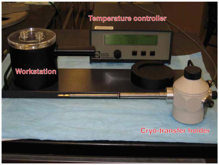
Cryo-transfer system overview. The components of the cryo-transfer system include the cryo-transfer holder, the transfer workstation and the temperature controller.
Figure 3.
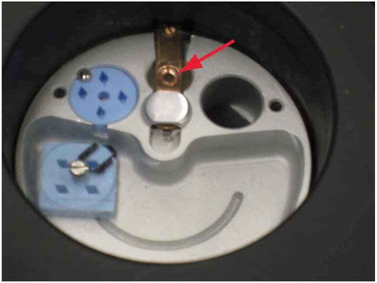
Cryo-transfer station. The tip of the cryo-transfer holder can be seen in the liquid-nitrogen-filled transfer vessel (red arrow). The box containing the frozen-hydrated grids is loaded into the station (blue boxes). The grid is transferred from the storage box to the cryo-holder in a liquid-nitrogen-cooled environment.
Figure 4.
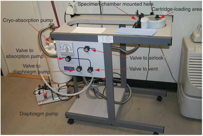
Polara transfer station overview: The labeled photo shows the individual parts of the transfer station.
Figure 5.
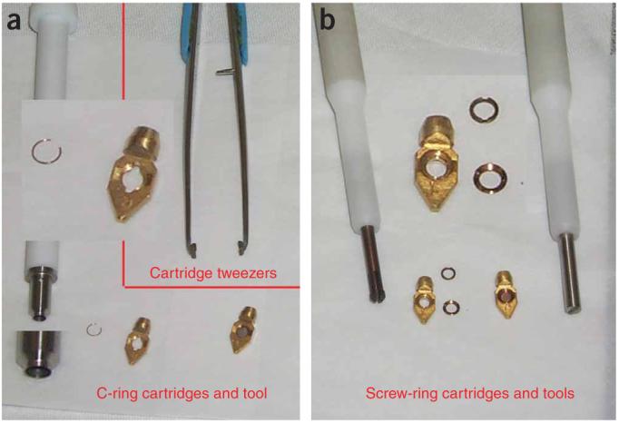
Tools and cartridges. (a) Image shows the c-ring cartridges, the ring insertion tool and the special cartridge tweezers. (b) Image shows the screw-ring cartridges, the screw rings and the drivers used to secure the sample into the cartridges.
Figure 6.
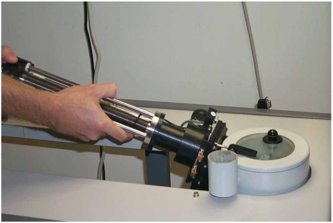
MSC being mounted on transfer station.
Figure 7.

The transfer station. (a) Transfer station pumping block: various valves that are manipulated during venting and evacuation of MSC are shown. (b) MCS and transfer station valves. Red arrow indicates Va (MSC valve), blue arrow indicates gate valve (station valve) and green arrow indicates plug to release lock.
Figure 8.
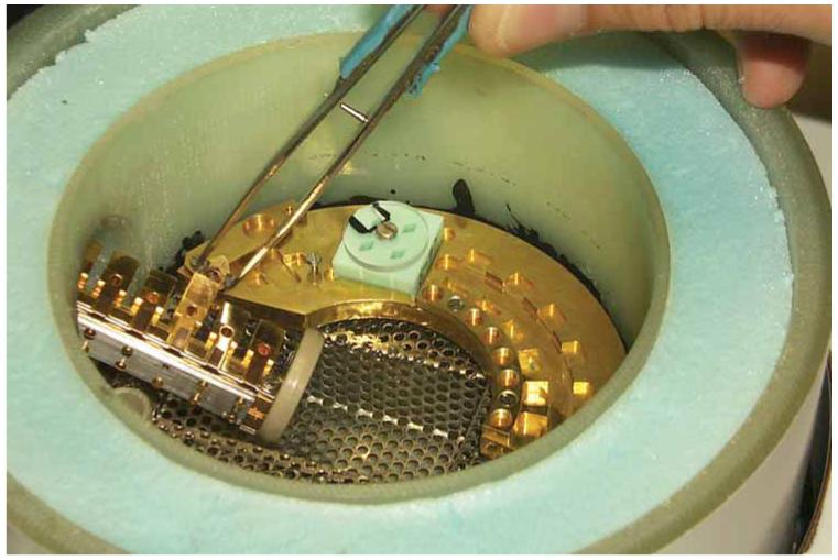
Transfer vessel with MSC inserted. The six ‘parking’ positions can be seen along with a cartridge being transferred into position 3 with the special cartridge tweezers (for more clear viewing, liquid nitrogen is not used in this image).
Figure 9.
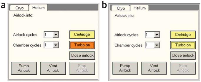
Turbo. (a) Waiting for turbo: vacuum UI Helium tab while turbo has not yet reached operating speed (orange color). (b) Turbo at operating speed: the turbo pump has reached operating speed (yellow color) and is ready for pumping. Reproduced with permission by FEI.
Decide on a data collection strategy
2| Before data are collected, there are several strategic decisions that need to be made. The two main questions to be answered are (i) whether or not a reference is available for reference-based alignment and orientation assignment of the projections (Box 1) and (ii) whether the data will be collected on a film or with a CCD camera (Box 2, Table 1). If a preliminary structure can be used as a reference, data collection can be done using single ‘untilted’ images (i.e., with untilted specimen stage; see ref. 5) as given in option A. If no such reference is available, a preliminary reconstruction must first be calculated as described in option B, either by the random-conical method6 or by common lines7,8 (see Box 1). The choice of which detector should be used is determined by the level of automation that is desired and the target resolution. Details such as pixel size, magnification, etc. are also discussed.
BOX 1 | RANDOM-CONICAL AND COMMON-LINES METHODS FOR DATA COLLECTION.
Random conical
For random-conical data collection, micrographs are taken as tilt pairs8. Following this strategy, two pictures are taken of the same area, the first at a high tilt value (∼55°) and the second untilted (0°). The first tilted image is used for a conical reconstruction based on the orientation determined using the untilted second image.
Common lines
For common lines, data are collected the same way as if a reference was available (see Box 5). Subsequent processing steps, however, are different, as described in refs. 10 and 11.
BOX 2 | CHOICE OF DETECTOR.
The selection of which detector to use is based on considerations such as target resolution, convenience and efficiency of data collection. Data can be collected manually (i.e., each image area is selected based on visual criteria) or using automated data collection programs12,13. Table 1 illustrates a few examples of the most commonly used recording media.
Resolution is defined as the ability to distinguish two features that are at a certain distance from each other. The smallest space a feature can occupy on film (option A) or a CCD (option B) is 1 pixel; so the maximum resolution (the closest two features can be from each other) is 2 pixels. On the object scale, the pixel size is set by the magnification of the image projected onto a detector with a fixed minimum pixel size (see Table 1). As the magnified projection of the object onto the detector increases, the object-scale area represented by the pixel decreases. The field of view, therefore, decreases with increasing magnification, so the number of particles per image collected decreases. For these reasons, the magnification used for data collection needs to be set accordingly. Some examples of practical settings for magnification and pixel sizes used in this lab, along with the current information limits, can be seen in Table 1.
(A) Film
An advantage of collecting data with film is that it allows a large field of particles at a finely resolved pixel size to be collected in a single micrograph. For example, one micrograph can contain up to 1,000 ribosome-sized (25 nm diameter) particles when a magnification of ×50,000 is used. A disadvantage of using film is that it must be physically inserted into, and removed from, the electron microscope, then processed in a darkroom and digitized before the data can be processed.
(B) CCD camera
The advantage of a CCD camera is that it produces immediate feedback and enables efficient, automated collection of a large amount of data. The disadvantage, compared to using film, is that the magnification must be increased (doubled in the above description) to achieve the same pixel size on the object scale. As a consequence, an image collected with a 4 K × 4 K CCD camera may represent less than one-fourth of the area collected with film. Thus, at a set pixel size, the total number of particles collected on the CCD is only one-fourth of that collected on film.
TABLE 1.
List of practical values when film or CCD is used as recording medium
| Detector | Minimum sampling size | Low-dose pixel | Area captured per exposure (object scale) | Practical information limit |
|---|---|---|---|---|
| Film | 7 μm (scanned) (3,629 dpi) | 1.2 Å at ×59,000 magnification | 1.2 μm × 1.38 μm | 3.6 Å (3 pixels) |
| CCD | 15 μm (CCD pixel) | 1.5 Å at ×100,000 magnification | 0.614 μm × 0.614 μm | 7.5-10 Å (>4 pixels) |
- With reference
- Low-dose micrographs are collected at defined defoci. These micrographs will later be grouped according to their defocus values for separate reconstructions. The contrast-transfer functions associated with the resulting density maps will then be corrected and subsequently combined. The individual micrographs must have sufficient contrast to allow the individual particles to be picked and properly sorted by orientation. The defocus range used for our data is usually from 1.5 to 4.0 μm underfocus in 0.25 μm increments.
- Without reference
- If a reference is not available, select which strategy to use: random conical or common lines, for subsequent processing, and follow the protocol associated with that option.
3| Select the detector after referring to Box 2 and Table 1 for guidelines.
Electron-optical settings
4| Set up the microscope for data collection according to the considerations described in Boxes 3 and 4.
BOX 3 | AVOIDING CONTAMINATION.
Maintaining a clean vacuum in the microscope column is critical to avoiding conditions that will degrade performance. This is especially true with cryo-samples as contaminants will build up on their cold surface if not kept away.
▲ CRITICAL Introduction of contaminants can also be avoided with proper precautions when loading a sample into the microscope or when exchanging a plate camera. Minimizing the time that cold tools and the cryo-sample are exposed to ‘wet’ air will reduce the relatively large-size ice contamination. Contamination build-up rates can be reduced to as little as 0.24 nm h-1 using very dry film and 0.13 nm h-1 if no film is used (CCD)14. Examples of the type of contaminants that can be introduced can be seen in the Troubleshooting section of the companion article1.
BOX 4 | ELECTRON-OPTICAL SETTINGS.
Before recording images, an electron-optical alignment is first carried out to optimize the performance of the microscope.
A good alignment procedure ensures that the path the electron beam traverses is directly along the optical axis. This alignment will minimize defects that can cause loss of resolution, such as axial astigmatism, in the experimental data. The choice of accelerating voltage is determined by the particle size, composition and the desired resolution. Most cryo-EM data in this lab are collected at a voltage between 100 and 300 kV using a high-brightness field-emission electron source for increased coherence. Higher voltage is necessary when aiming for highest resolution, but it entails a decrease in contrast.
Low-dose setup
5| Set up the low-dose kit according to the considerations described in Box 5 (Fig. 10) and Table 2, and the following steps.
BOX 5 | LOW-DOSE SETUP.
The low-dose kit (FEI) allows the user to minimize the amount of electron dose that a beam-sensitive biological sample is exposed to. This is accomplished by using low magnification for viewing the grid square and to survey areas where data will be collected (search mode, ∼ ×3,000). Accurate focusing of the image is accomplished by applying a defined amount of beam/image shift at high magnification (×115,000) to an area that is a set distance away from the optical axis (focus mode). The beam shift allows focusing of the image on an area adjacent to the hole where the data will be collected (Fig. 10). Once accurate focusing is complete, an exposure can be taken without image or beam shift at the magnification (∼ ×50,000) and dose required (20 eÅ-2, 300 kV; exposure mode). The magnification for the exposure mode is determined as described in the electron-optical settings section in PROCEDURE, and some examples of dose-magnification-kV-defocus combinations are given in Table 2. The illumination settings and exposure time must be such that the detector is fully illuminated and the exposure time is sufficiently short (∼1 s) to minimize potential effects from specimen drift.
An image in exposure mode is taken on the optical axis. It defines the conditions under which data will be collected. The detector that will be used to visualize the grid—fluorescent screen, CCD camera or film (only in exposure mode)—is set for each of the low-dose modes (see Fig. 11).
Figure 10.
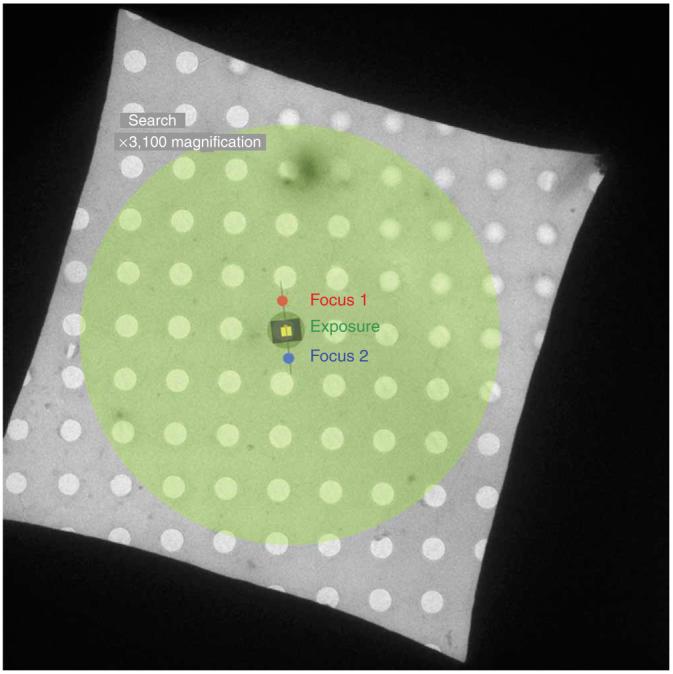
Diagram of grid square showing various low-dose areas. The areas exposed during the various low-dose modes are represented by colored circles on the EM grid square. Search mode (large green circle) is obtained at approximately ×3,000 magnification to minimize electron dose. Focus mode (red and blue circles) is off-axis and performed at about ×100,000 magnification. Exposure mode (dark green circle covering the center hole) is commonly taken at ×39,000-×100,000 when data are collected. The black rectangle represents the area covered by film and the yellow square represents the area covered by a 4KX4K CCD camera.
TABLE 2.
Practical combinations of magnification, accelerating voltage, dose and defocus range
| Magnification | Dose | Defocus range |
|---|---|---|
| ×50,000 | 10 e Å-2 (100 kV) | 0.7-2.5 μm |
| ×50,000 | 20 e Å-2 (200 kV) | 1.2-3.0 μm |
| ×59,000 | 25 e Å-2 (300 kV) | 2.0-4.0 μm |
| ×39,000 | 15 e Å-2 (300 kV) | 2.0-4.0 μm |
6| Center the stage and load a non-cryo holey carbon grid for low-dose set up (This can also be done with a grid that is already loaded).
7| Set the eucentric height using the alpha wobbler feature to rock the stage ± 15°. The stage is at the eucentric Z position when there is little or no movement as the stage rocks back and forth.
8| Activate the low-dose program by clicking the ‘low-dose’ button in the UI (see Fig. 11).
Figure 11.
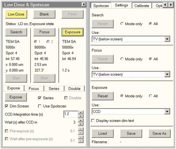
Low-dose UI. The low-dose program is activated by clicking on the ‘low-dose’ button. The yellow color of the button indicates that the low-dose program is active. Detector selection is available in the right half of the UI. Reproduced with permission by FEI.
9| Select the desired C1 (spot size) setting and C2 aperture.
! CAUTION It is best if the spot size is the same for all modes (search, focus, exposure) to avoid the effects of hysteresis when switching between modes. The greatest effect of hysteresis is misalignment of the beam causing partial exposure of the detector.
10| Find an easily recognizable feature that can be seen in search mode, but is small enough that it (or a distinct feature, such as a corner) can still be identified in exposure and focus modes.
11| Go to exposure mode and center the feature, or a distinct corner of the feature, using the stage controls. Adjust the illumination size to the desired level.
12| Go to search mode and center the same feature using image shift. The center of search mode is now aligned with the center of the image in exposure mode.
13| Go to exposure mode and move the feature just off of the large fluorescent screen with the stage controls along the tilt axis direction.
▲ CRITICAL STEP Note that the tilt axis (determined visually) is coincident with the long axis of the stage. Shift in the direction of the tilt axis is of critical importance if data collection from a tilted sample is considered, to avoid a change in Z position (and thereby defocus) between focus and exposure modes.
14| Go to focus mode position 1 by clicking ‘Focus’ in the low-dose UI (see Fig. 11).
15| If the feature of interest is visible, center it by applying image shift with the multifunction knobs and beam shift with the left track ball.
▲ CRITICAL STEP If the feature is not visible, decrease the magnification and spread the beam until the feature becomes visible, then center the feature as described previously. Reset the magnification and focus the beam to the desired level.
16| Go to exposure mode and center the recognizable feature with the stage controls. Move the feature with the stage control just off the large fluorescent screen in a direction opposite to what was done in Step 13.
17| Go to focus mode position 2 and repeat Step 11.
▲ CRITICAL STEP The ‘opposite’ direction from focus position 1 can also be set by adding 180° to the direction set in focus position 1.
18| Select the detector to be used for each mode (see Fig. 11).
19| Enter the exposure time that will give the desired dose for the exposure. See Table 2 for an approximation of these settings.
20| Go to search mode and activate the beam blanker by clicking on the ‘blank’ button in the UI (see Fig. 11).
21| Save the low-dose settings by clicking the ‘save’ button in the UI (see Fig. 11).
22| Close the column valves (if available in the microscope used) and remove the grid (if other than grid to be used for data collection) that was used for setup.
23| Insert the cryo-sample by following the protocol for the specific holder and microscope being used (if applicable).
Collecting data under low-dose conditions
24| Once the sample is inserted, the vacuum has recovered and the sample temperature has stabilized, data collection can begin.
25| Open the column valves (if available in the microscope used) and deactivate the low-dose beam blanker.
26| Survey the grid in search mode and record the squares desired for data collection using the stage UI. Good areas with thin ice can be determined using a CCD camera, measuring the relative beam intensity, or by visual inspection by the user.
27| Once the good grid squares have been recorded for data collection, center a good hole in search mode and go to exposure mode. This will be your ‘sacrificial hole.’ If necessary, adjust the beam position and diameter.
28| Go to focus mode and focus the image.
29| Go to search mode and move to the center of an adjacent good hole.
30| Go to focus mode and focus the image. Set the desired defocus.
31| Wait for the drift to decrease below at least 0.5 nm s-1 or when there is no visible movement at the focus mode magnification (∼ ×100,000).
32| Take an exposure using the selected detector.
33| Go to exposure mode and check the illumination and hole position. Adjust if necessary.
34| Go to focus mode and then to search mode to select the next good hole.
▲ CRITICAL STEP Following the sequence of search-focus-expose-focus will minimize beam and image shifts caused by hysteresis.
35| Traverse the grid square in a regular pattern that will avoid pre-irradiating unexposed areas.
36| When the grid square is exhausted, move to the next ‘good’ grid square and continue data collection as above.
37| When the disk is filled or the plate stock (film cassette) is exhausted, activate the beam blanker and close the column valves (if available in the electron microscope used; if not, see Box 6).
BOX 6 | NO COLUMN VALVES.
Most FEG microscopes have ‘column valves’ to protect the gun, but non-FEG instruments may not. If this is the case, the protocol given below applies.
Turn off HT and turn down filament heating to protect filament while venting the camera.
Exchange the exposed camera with an unexposed one.
Turn the HT back on and saturate the filament slowly.
38| Perform the steps in option A if you are using film, or proceed to option B if capturing the images using CCD.
- If film is used
- Vent the camera click on the ‘vent camera’ button and confirm in the vacuum UI.
-
Once the projection chamber reaches atmospheric pressure, remove the camera with the exposed film and replace it with a new camera with an unexposed film.▲ CRITICAL STEP The new camera must be well desiccated to prevent it from adversely impacting the microscope vacuum level or increasing contamination rates (see Box 3).
- Click pump camera to evacuate the projection chamber. Note that the time needed for the vacuum to recover is generally about 30 min unless the camera has not been sufficiently desiccated, in which case thetimewill belonger.
- Bring the exposed camera to the dark room.
- Turn on the safe lights (Kodak 1 or GBX-2 safelight filter) and turn off the white lights.
- Remove the exposed film from the cassettes and load it into developing racks.
- Develop the low-dose film for 12 min in full-strength Kodak D19 at 20 °C with nitrogen burst agitation.
- Move the film into a circulating water bath to wash and stop the developing for 1 min.
- Transfer the film into Kodak Rapid fixer for 4.5 min.
- Remove from the fixer and wash in circulating water bath for 1 h.
- Dip the plates in a Kodak Photo-flo solution to prevent the formation of water spots.
- Place in film dryer (35 °C) for 1 h or on shelf at room temperature (20-25 °C) for 5 h to dry.
- Digitize the film with available high-resolution scanner for later data processing.
- If data are collected on CCD
-
Transfer the data from the microscope disk (C:) to a separate network mounted drive. Ensure that there is enough disk space for further data collection.▲ CRITICAL STEP The disk that contains the EM control software (C:) must be kept free of clutter to ensure optimal performance.
-
39| Repeat Steps 29-37 until data collection is complete.
Exit low-dose mode
40| When data collection is complete, go to search mode. If desired, save the low-dose conditions in a file for future use.
41| Deactivate the low-dose program.
42| Center the stage.
43| Close the column valves (if available in the microscope used; if not, see Box 6).
44| Remove the sample. If data collection is over, start the cryo-cycle to protect the ion-getter pumps (if available in the microscope used).
ANTICIPATED RESULTS
Visualization of correctly prepared cryo-EM grids using this protocol should produce images of sufficient quality to achieve 3D reconstructions with resolutions in the 1-2 nm range, assuming high sample homogeneity, when processed with single-particle techniques9 (see Fig. 12).
Figure 12.
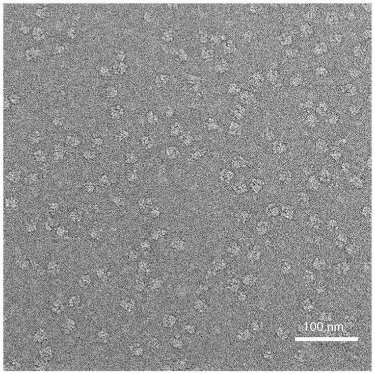
Micrograph of ribosomes in vitreous ice. The micrograph shows an even particle distribution of ribosomes on a frozen-hydrated grid. Note that contrast has been inverted for subsequent image processing.
ACKNOWLEDGMENTS
We acknowledge the support from HHMI, NIH R37 GM29169, R01 GM55440 and P41 RR01219. We also thank M. Watters for assistance in generating figures.
References
- 1.Grassucci RA, Taylor DJ, Frank J. Preparation of macromolecular complexes for cryo-electron microscopy. Nat. Protoc. 2007;2:3239–3246. doi: 10.1038/nprot.2007.452. [DOI] [PMC free article] [PubMed] [Google Scholar]
- 2.Frank J. Three-Dimensional Electron Microscopy of Macromolecular Assemblies: Visualization of Biological Molecules in Their Native State. Oxford University Press; New York: 2006. [Google Scholar]
- 3.Dubochet J, Lepault J, Freeman R, Berriman JA, Homo J-C. Electron microscopy of frozen water and aqueous solutions. J. Microsc. 1982;128:219–237. [Google Scholar]
- 4.Wagenknecht T, Carazo JM, Radermacher M, Frank J. Three-dimensional reconstruction of the ribosome from Escherichia coli. Biophys. J. 1989;55:455–464. doi: 10.1016/S0006-3495(89)82839-5. [DOI] [PMC free article] [PubMed] [Google Scholar]
- 5.Spahn CM, et al. Hepatitis C virus IRES RNA-induced changes in the conformation of the 40S ribosomal subunit. Science. 2001;291:1959–1962. doi: 10.1126/science.1058409. [DOI] [PubMed] [Google Scholar]
- 6.Valle M, et al. Incorporation of aminoacyl-tRNA into the ribosome as seen by cryo-electron microscopy. Nat. Struct. Biol. 2003;10:899–906. doi: 10.1038/nsb1003. [DOI] [PubMed] [Google Scholar]
- 7.Halic M, et al. Structure of the signal recognition particle interacting with the elongation-arrested ribosome. Nature. 2004;427:808–814. doi: 10.1038/nature02342. [DOI] [PubMed] [Google Scholar]
- 8.Radermacher M, Wagenknecht T, Verschoor A, Frank J. Three-dimensional reconstruction from a single-exposure, random conical tilt series applied to the 50S ribosomal subunit of Escherichia coli. J. Microsc. 1987;146:113–136. doi: 10.1111/j.1365-2818.1987.tb01333.x. [DOI] [PubMed] [Google Scholar]
- 9.Taylor DJ, et al. Structures of modified eEF2 80S ribosome complexes reveal the role of GTP hydrolysis in translocation. EMBO J. 2007;26:2421–2431. doi: 10.1038/sj.emboj.7601677. [DOI] [PMC free article] [PubMed] [Google Scholar]
- 10.Penczek PA, Zhu J, Frank J. A common-lines based method for determining orientations for N > 3 particle projections simultaneously. Ultramicroscopy. 1996;63:205–218. doi: 10.1016/0304-3991(96)00037-x. [DOI] [PubMed] [Google Scholar]
- 11.Van Heel M. Angular reconstitution: a posteriori assignment of projection directions for 3D reconstruction. Ultramicroscopy. 1987;21:111–123. doi: 10.1016/0304-3991(87)90078-7. [DOI] [PubMed] [Google Scholar]
- 12.Lei J, Frank J. Automated acquisition of cryo-electron micrographs for single particle reconstruction on an FEI Tecnai electron microscope. J. Struct. Biol. 2005;150:69–80. doi: 10.1016/j.jsb.2005.01.002. [DOI] [PubMed] [Google Scholar]
- 13.Suloway C, et al. Automated molecular microscopy: the new Leginon system. J. Struct. Biol. 2005;151:41–60. doi: 10.1016/j.jsb.2005.03.010. [DOI] [PubMed] [Google Scholar]
- 14.Ohi M, Li Y, Cheng Y, Walz T. Negative staining and image classification— powerful tools in modern electron microscopy. Biol. Proced. Online. 2004;6:23–34. doi: 10.1251/bpo70. [DOI] [PMC free article] [PubMed] [Google Scholar]