Choice and Interpretation of Statistical Tests Used When Competing Risks Are Present

Abstract

In clinical cancer research, competing risks are frequently encountered. For example, individuals undergoing treatment for surgically resectable disease may experience recurrence near the removed tumor, metastatic recurrence at other sites, occurrence of second primary cancer, or death resulting from noncancer causes before any of these events. Two quantities, the cause-specific hazard function and the cumulative incidence function, are commonly used to summarize outcomes by event type. Tests for event-specific differences between treatment groups may thus be based on comparison of (a) cause-specific hazards via a log-rank or related test, or (b) the cumulative incidence functions via one of several available tests. Inferential results for tests based on these different metrics can differ considerably for the same cause-specific end point. Depending on the questions of principal interest, one or both metrics may be appropriate to consider. We present simulation study results and discuss examples from cancer clinical trials to illustrate these points and provide guidance for analysis when competing risks are present.

INTRODUCTION

When individuals undergo treatment for cancer, in most cases there are a variety of possible subsequent outcomes. For example, although radiotherapy after surgical removal of a tumor is administered for local control, distant metastases may appear first. Chemotherapy may be administered to reduce distant recurrence, but second primary cancer or treatment-related mortality may occur first. When we define the primary outcome specifically as the occurrence of one of these events, a competing risks problem is created.

In these situations, constraints dictated by the mathematical results of competing risks theory determine which quantities can be estimated. Ideally, we would like to know the marginal or “net” probability of failure caused by a given event type, which pertains to the probability of failure resulting from that event in the absence of the other failure types. This is a hypothetical quantity because it depends on (usually) unknown information about the interdependence between the event of interest and other events, and thus we cannot reliably test hypotheses concerning it.^1-4 However, we can estimate quantities pertaining to the probability of failure caused by an event of interest under the study conditions at hand; that is, when other failure types may preclude it. In recent years, numerous articles have addressed what can be correctly estimated with competing risks data, with many using examples from cancer research.^5-10

Although much has been written regarding estimation in competing risks situations, less attention has been devoted to hypothesis testing. In many cases, the choice of test may be unclear, and substantively different inferential conclusions (ie, P values) will arise from the same data depending on which test is used. These seeming discrepancies naturally occur because the tests address different aspects of the failure process, one or more of which may be of interest in a given situation. In this article, we use data from a phase III clinical trial and simulation studies to illustrate when and why competing risks tests differ, and offer guidance for the use of these methods.

BACKGROUND: COMPETING RISKS OBSERVATIONS AND ESTIMABLE QUANTITIES

Observations

In the competing risks setting, an individual can potentially experience failure from any of several, say K, event types, but we observe the time to failure for the first event (or the last follow-up time if no failure has occurred). Even in cases where individuals can have multiple events (eg, local followed by distant failure), we can still designate one event as occurring first, creating competing risks observations. This is often desirable because after the first failure, interventions are likely to change, and although there are methods for analyzing multiple events per patient, the additional analytic complexity required often does not yield materially different information. Note that even when only one event is observed per patient, we have partial information on all failure types. For example, if the patient experienced failure as a result of cause 1 at T = 40 months, it is known that were he/she to experience it, the patient's time to failure due to cause 2 would be at least 40 months. Practical implications of this depend on the specific context. For example, distant metastases may indeed occur after local failure, whereas time of local or distant failure once an individual has died is strictly a hypothetical construct.

Cause-Specific Hazard Functions

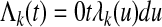
The principal estimable quantity in competing risks is the cause-specific hazard function λ_k(t), which can heuristically be thought of as a probability of failure specifically resulting from cause k in a small interval of time, given that no failure of any kind has occurred thus far. The overall hazard λ(t) for any type of failure at time t is the sum of the cause-specific hazards λ_k(t). The cumulative cause-specific hazard function Λ_k(t) or cumulative hazard function Λ(t) equals the value of its corresponding hazard function summed up to time t. Note that the cumulative hazard function is uniquely related to the familiar survival function (probability of survival past time t) via S(t) = exp(–Λ(t)). However, exp(–Λ_k(t)) is in general not interpretable as the survival function for cause k alone unless additional assumptions are made that cannot be verified in competing risks data.^1-4

Average Hazard Rates

Average hazard rates are computed simply as the number of events of type k divided by sum of the total follow-up times (to their first event or censoring) over all individuals, or the person-time at risk. Conveniently, these rates are additive to the average hazard rate for failure from any cause.

Cumulative Incidence Functions

Cumulative incidence is defined as the cumulative probability of event k having occurred in the presence of other competing events. It is expressed mathematically as

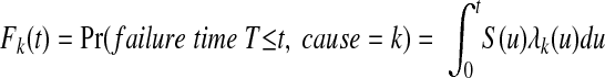Heuristically, this expression shows that the cumulative incidence of event k is a function of both the probability of not having failed from some other event first (S(u)) up to time t and the cause-specific hazard for the event of interest (λ_k(u)) at that time.^5-10 At any time point, the K cumulative incidence functions are additive to the probability of failure resulting from any cause.

The cumulative probability of event k occurring in the presence of competing risks is often incorrectly estimated by 1–S_k(t), where S_k(t) is calculated (via the Kaplan-Meier estimator) treating events other than those resulting from cause k as censored observations. This estimator does not properly take into account the probability of remaining at risk for cause k at time t (ie, not experiencing failure resulting from other causes before t), and consequently overestimates the cumulative event-specific probability.^4-10

Inference for Competing Risks Data

When comparing two groups with respect to failures for one event type in the face of competing events, several options are available. We concentrate here on two widely used tests, the first for cause-specific hazards and the second for cumulative incidence functions.

Log-rank test for hazards.

The log-rank test is widely used in survival analysis to evaluate differences between groups.¹¹ Briefly, failure times are ordered from smallest to largest, and the data are organized into 2 × 2 tables of group (A or B) by failure (yes or no) at each time. The log-rank test sums over these tables the difference between the observed failures and the failures expected if the two groups had equal probability of failure, producing a statistic that reflects differences in the failure experience between groups over the entire follow-up time. As individuals either fail or are censored over time, the pool of individuals remaining, or the risk set, is diminished. Tests of this type are used to “compare survival curves” when in fact they essentially compare the underlying hazards.

When there are K ≥ 2 possible types of failure and we wish to compare the two groups with respect to the cause-specific hazard for failure cause k, we can compute the log-rank test as above, censoring events resulting from causes other than k. That is, the individual exits the risk set once the competing event occurs, the same way they would if they reached the end of their follow-up with no event observed. This fact has some bearing on interpretation of differences in cause-specific hazards if events are interdependent, as discussed later herein. Furthermore, the attrition resulting from competing failures may be more likely to occur unequally between groups, affecting statistical power.¹²

Gray's test for subdistribution hazards.

A number of tests have been proposed for comparing cumulative incidence functions,^9,13 but the first and perhaps the most frequently used is that by Gray.¹⁴ Gray's test is used to evaluate hypotheses of equality of cause-specific cumulative incidence functions between two groups, but as in the case of comparing survival curves, the test actually compares an underlying function of the cumulative incidence function, namely the subdistribution hazard. The subdistribution hazard can be thought of as the hazard of an artificial time variable T′ defined as T′ = T if a failure resulting from cause k occurred and T′ = ∞ if other failure types occurred.^14,15 In the absence of censoring, Gray's test is identical to the log-rank test computed using T′ as the time variable.¹⁴

This fact points to how the log-rank test and Gray's test differ. Suppose we have a primary failure cause 1 and a competing failure cause 2 for two treatment groups A and B and wish to test whether the groups differ with respect to occurrence of event 1. Suppose the first failure is a result of cause 1 in group A. The log-rank and Gray's test statistics at this failure time are identical. Then, suppose that between the first and second failure times resulting from cause 1, a failure resulting from cause 2 occurs in treatment group B. For the log-rank test, that individual exits the risk set, whereas in Gray's test, with respect to event 1, such an individual remains in the risk set forever, indicated by the cause 1 failure time becoming T′ = ∞. Thus, the two test statistics will differ starting at the next cause 1 failure. This fundamental difference in how competing events are handled in the computation of the test statistics will result in different inferential conclusions, even when cause-specific hazards of failure resulting from cause 1 are identical in the two groups.

Additional technical details of statistical methods in competing risks appear in the Appendix (online only). In the application and simulated data examples that follow, we illustrate how these summaries and tests reveal different aspects of competing risks observations.

APPLICATION: BENEFICIAL AND ADVERSE EVENTS WITH TAMOXIFEN TREATMENT FOR BREAST CANCER

In early-stage breast cancer, competing risks are ubiquitous because after successful removal of the primary tumor, patients encounter risk of disease recurrence, onset of second primary cancers, adverse medical events attributable to adjuvant treatment, or death resulting from noncancer causes. To evaluate the antiestrogen tamoxifen in early-stage breast cancer, the National Surgical Adjuvant Breast and Bowel Project (NSABP) Protocol B-14 trial opened in 1982 and randomly assigned more than 2,800 women to 5 years of either tamoxifen or placebo after surgery for estrogen-receptor–positive breast tumors.^16,17 Primary trial end points were (a) disease-free survival (DFS), defined as time to the first of any of the following: breast cancer recurrence, second primary cancer (including contralateral breast tumors), or death preceding any of these events; and (b) mortality from any cause. Among the events comprising DFS, primary interest is in recurrence and contralateral tumor reduction with tamoxifen. However, the extent of excess risk for endometrial cancer or other events (other second cancers and noncancer deaths) for women taking tamoxifen is also of clinical relevance.

Figure 1A shows the cumulative cause-specific hazard by treatment group for each of four mutually exclusive (first) event types. In large data sets such as this, where the number of events is small relative to the number of patients at risk, the cause-specific hazards resemble probabilities, but we note that the cumulative hazard is not strictly a probability and does not have a direct clinical interpretation as such. Figure 1B shows the cumulative incidence of these events, which does equal the cumulative probability of occurrence of each event type in the presence of competing events. At each time point, these cumulative incidence function are additive to the probability of failure from any of the potential causes (ie, equal to 1–DFS).

Fig 1.

(A) Cumulative cause-specific hazard and (B) cumulative incidence of events comprising disease-free survival in a clinical trial for lymph node–negative, estrogen-receptor–positive breast cancer.¹⁶,¹⁷ Vertically from top, graph pairs represent breast cancer recurrence, contralateral breast tumors, endometrial cancer, and other events.

Heuristically, the log-rank and Gray's tests can be thought of as comparing groups with respect to cause-specific hazards or cumulative incidence functions in Figure 1 over the entire follow-up time. Table 1 shows these tests along with other relevant summaries of outcomes between groups. The average hazard rates for each event type and for any event, or DFS (bottom row) provide a sense of the magnitude of failures per year. Also shown are ratios between groups of the average hazard rates, which can provide a useful index of the relative difference in event risk between the two groups. More commonly, a similar quantity, the hazard ratio (HR), would be obtained via the Cox proportional hazards model,¹⁸ which in this case provides an estimate similar to this simple summary (data not shown). Estimated cumulative incidence for the events by treatment group at the 12-year landmark is also shown.

Table 1.

Average Hazard Rates, Average Hazard Rate Ratios, Log-Rank Test, and Gray's Test for Events Comprising Disease-Free Survival in a Clinical Trial of Tamoxifen for Node-Negative, Estrogen-Receptor–Positive Breast Cancer¹⁶,¹⁷

Event Type	Placebo		Tamoxifen		Rate Ratio	95% CI	12-Year Cumulative Incidence				P
	No. of Events	Rate*	No. of Events	Rate*			Placebo		Tamoxifen		Log Rank	Gray's
							%	95% CI	%	95% CI
Recurrence	437	32.17	276	18.10	0.56	0.48 to 0.66	29.2	26.8% to 31.6%	18.2	16.2% to 20.2%	< .0001	< .0001
Contralateral breast tumor	105	7.73	81	5.31	0.69	0.51 to 0.93	6.5	5.1% to 7.9%	4.5	3.3% to 5.7%	.0108	.0687
Endometrial cancer	6	0.44	30	1.97	4.46	1.82 to 13.09	0.4	0.0% to 0.8%	1.8	1.0% to 2.6%	.0003	.0001
Other events	175	12.88	212	13.91	1.08	0.88 to 1.33	10.1	8.5% to 11.7%	11.9	10.1% to 13.7%	.5551	.0409
All first events (disease-free survival)	723	53.22	599	39.29	0.74	0.66 to 0.82	46.2	43.6% to 48.8%	36.3	33.8% to 38.8%	< .0001	—

^*Average annual rate per 1,000 patients.

For breast cancer recurrence, the hazard is significantly reduced among women randomly assigned to tamoxifen (log-rank P < .0001), and cumulative incidence of recurrence is also highly significantly lower (Gray's P < .0001). The approximate 31% relative reduction in hazard of contralateral breast tumors in the tamoxifen group reaches conventional statistical significance (log-rank P = .01), whereas the absolute decrease in incidence of 2% at 12 years does not (Gray's P = .0687). For endometrial cancer, a four-fold relative excess in hazard is seen for the tamoxifen group, and the absolute difference in cumulative incidence is approximately 1.4% at 12 years. In both cases the difference is highly statistically significant—for the hazard because a four-fold relative excess is indeed quite large, and for the cumulative incidence function because although the absolute difference is smaller than that for contralateral breast cancer; the relative increase in event probability is also on the order of a four-fold greater incidence.

Interestingly, for other events (second primary cancers and deaths as first event), the log-rank test indicates no difference, whereas Gray's test shows significant excess of these failures of approximately 1.8% at 12 years in the tamoxifen group. Unlike endometrial cancer, where a biologic mechanism supports the excess risk in the tamoxifen group, here the difference likely reflects the fact that many more individuals in the placebo group first have a recurrence or contralateral breast tumor, whereas in the tamoxifen group, relatively more individuals remain at risk for other cause failures, resulting in greater cumulative incidence of these events (Fig 1).

When all events are considered together, the net benefit for tamoxifen is considered highly favorable because recurrent breast cancer is frequent and poses a significantly greater mortality threat than endometrial cancer, whereas contralateral breast tumor risk is also reduced and other events do not appear to be directly influenced by tamoxifen. This is also the consensus opinion from a large body of clinical trials of tamoxifen.¹⁹ For suitably high-risk individuals, tamoxifen may even be considered for breast cancer incidence reduction, despite increased endometrial cancer risk.²⁰

SIMULATED DATA EXAMPLES

Studies of the relative performance of the log-rank and Gray's test have recently appeared in the statistical literature.^21-23 Here, we further illustrate the relationship between these tests using two examples. For two groups A and B, hypothetical follow-up times with two possible failure types (events 1 and 2) along with a random censoring time were generated from independent exponential distributions with different known hazard rates. The observed time is taken as the minimum of the two event times and the censoring time. We then used the log-rank and Gray's tests (at two-sided α = .05) to examine the differences between groups (Table 2). Corresponding cumulative hazard and cumulative incidence function plots are shown in Figure 2.

Table 2.

Comparison of the Log-Rank and Gray's Test Under Different Competing Risks Scenarios, With 500 Subjects per Group

Scenario	Hazards				Hazard Ratio	Log-Rank Probability (reject)	Gray's Probability (reject)
	Specified		Estimated
	Group A	Group B	Group A	Group B
I
Event 1	λ11 = 1.00	λ21 = 1.00	1.002	1.003	1.001	.048	.369
Event 2	λ12 = 1.00	λ22 = 1.50	1.002	1.501	1.498	.978	.941
Overall	—	—	2.004	2.504	1.250	.846	—
II
Event 1	λ11 = 1.00	λ21 = 0.80	1.002	0.802	0.801	.576	.059
Event 2	λ12 = 1.00	λ22 = 0.67	1.002	0.667	0.666	.969	.692
Overall	—	—	2.004	1.469	0.732	.986	—

NOTE. Competing risks data were simulated from two independent exponential failure distributions with the hazard parameters indicated and independent censoring that resulted in approximately 25% of lifetimes being censored. Averages of estimated parameters and proportion of times the tests reject the null hypothesis (ie, power) are based on 3,000 independent simulated data sets.

Fig 2.

Cumulative incidence and cumulative hazard plots from the simulated data examples. The estimated curves are based on large samples from distributions having the parameters specified in Table 2. (A, B) Scenario 1; (C, D) scenario 2.

Scenario I: Equal Hazards for Event 1, Greater Hazard in Group B for Event 2

The log-rank test comparing cause-specific hazards indicates no difference between groups for event 1 (produces a significant result approximately 5% of the time, the rate expected by chance), whereas Gray's test rejection rate is 0.369 (meaning that, of a large number of simulation runs, approximately 37% differed enough to be statistically significant). This occurs because a greater number of individuals experience failure resulting from event 2 in group B, and thus fewer remain available to experience event 1, which results in its decreased cumulative incidence. For event 2, there are large differences in both hazards and cumulative incidence (Fig 2B), as both tests indicate (Table 2). Note that the overall (ie, event-free survival) HR is less extreme (HR = 1.250) than that for event 2 alone (HR = 1.498), and consequently the log-rank test for a difference in overall hazards has lower power (rejects less often) than the cause-specific log-rank test.

With larger sample sizes, the log-rank test will maintain its 5% rejection rate for event 1 (the nominal α = .05 level), whereas power for Gray's test will increase because the cumulative incidence does indeed differ between the groups (Fig 2A). Both tests will achieve higher statistical power for event 2 because both hazards and cumulative incidence differ between groups.

Scenario II: Hazards for Both Events Are Smaller in Group B Than in Group A

Cumulative hazards (Fig 2C and 2D, bottom) reflect the smaller hazard within group B for event 2 than for event 1, as well as smaller hazards for both events in group B than in group A. However, cumulative incidence is eventually higher for event 1 in group B than in group A (Fig 2C, top), even though the hazard is lower. Furthermore, the crossing cumulative incidence curves for event 1 results in a test result of no difference for Gray's test (a weighted test¹⁴ may be more appropriate in this case, if one were interested in, say, early or late differences in cumulative incidence). For event 2, group B is more favorable with respect to both the hazard and cumulative incidence (Fig 2D). For the overall hazard, even though the hazard ratio is slightly smaller, the imbalance in events in favor of group B resulting from both cause-specific hazards being smaller in that group results in high power for the log-rank test.

This scenario is not unrealistic in cancer treatment; for example, adjuvant therapy for breast cancer reduces both local and distant recurrence. Because power is determined in part by the number of failures, the reduction in observed failures caused by competing risks must be considered during study design to ensure adequate statistical power for cause-specific outcomes.^24,25 Additional considerations relating to power involve how the hazards (log-rank test) or subdistribution hazards (Gray's test) differ over time.²⁵ Both tests examined herein are optimal when the HR or subdistribution ratio is constant over time, or satisfies the proportional hazards (subdistribution hazards) assumption. This is why, for example, power for Gray's test in scenario I, event 1 is lower than that for scenario II, event 2, even though the curves appear more discrepant in the former (Fig 2A, top). The latter case, showing a consistent difference throughout follow-up time, more closely resembles the proportionality condition.

OTHER CONSIDERATIONS

Dependent Competing Risks

In real-life situations, because we observe only the minimum failure time and at most one failure type, we cannot estimate the magnitude of dependence between failure times or even detect its presence.^1-3 Nonetheless, dependence between failure times may be present. For example, patients who experience local recurrence may be more likely to have distant metastatic recurrence, with the event times correlated. That is, had the patient not experienced failure resulting from one of these first, he/she likely would have soon experienced failure resulting from the other. As simulation studies have shown that if there is correlation between failure types, then both the log-rank and Gray's tests may be affected.^21-23 Nonetheless, when analyzing data with respect to first failure event, we must rely on functions of the observed cause-specific hazards for inference, which may be different from the true hazards in absence of other events or taking correlation into account.

Modeling Competing Risks Data

In randomized trials, adjustment for covariates is either not necessary or can be accomplished via stratified versions of these tests. In other situations, one may wish to model the relationship of patient and disease covariates to outcomes in the competing risks setting. Analogous to the tests discussed in this article, one must consider the metric on which to model and interpret the results. For example, the familiar Cox model can readily be adapted for the cause-specific hazard, but the covariate effects obtained do not then pertain to the cumulative incidence of a given event type.^5,15,26 Additional issues with interpretation of covariates on the hazard scale may also arise.^27,28 When modeling on the cumulative incidence scale, one must keep in mind that cumulative probabilities are a function of multiple cause-specific hazards, and thus so are the regression coefficients. Modeling of cumulative incidence functions has been approached in a variety of ways, and methodology is still evolving.^15,29-31

DISCUSSION

Because, as Gray originally pointed out,¹⁴ cause-specific hazards and cumulative incidence curves capture different aspects of the event histories in competing risks data, inference on these metrics may yield different results. In this article, we have attempted to illustrate where and why this occurs. With respect to performance of the tests, the log-rank test correctly detects differences in cause-specific hazards, and, unless there is strong dependence between failure times, is largely unaffected by between-group differences in hazards for other competing events. On the other hand, Gray's test correctly detects whether there is a difference in cumulative incidence between groups for a given event, whether that difference is caused by a difference in hazards between the groups for the event itself or by a difference in hazards for the competing events. As the simulations illustrate, there are situations where the cumulative incidence curves and Gray's test will indicate, for example, that a treatment is beneficial with respect to one event type, when in fact the treatment has simply increased the incidence of a competing event. Thus, when choosing and interpreting a statistical test, one must take these properties into account, as well as whether primary interest is in contrasting the relative rate of events or the absolute difference in incidence of events between groups.

In clinical situations, competing events are often not strictly mutually exclusive, and so the relative consequences of each, as well as adverse and beneficial effects of subsequent interventions, must be considered. In the case of tamoxifen and endometrial cancer among breast cancer patients, the risk/benefit ratio is highly favorable, because if endometrial cancer occurs, it is likely to be detected early and be treatable. If the breast cancer recurs, the patient will likely discontinue tamoxifen and undergo additional, more aggressive treatments, so the risk of subsequent endometrial cancer may no longer be a major concern relative to the clinical situation at hand. A contrasting risk/benefit scenario might involve the occurrence of acute myelogenous leukemia (AML) and similar conditions after chemotherapy for breast cancer. Risk of AML appears to be associated with chemotherapy in a dose-dependent manner, with a six-fold relative risk increase for the highest-intensity dose compared with the standard regimen.³² Because AML is difficult to treat successfully, its occurrence either before or after breast cancer recurrence is of great clinical consequence. Even here, one must place the risk in the proper context; in the AML study,³² incidence reached about 1.25% at 8 years in the highest intensity chemotherapy arm, compared with 0.50% in the standard chemotherapy arm, whereas the absolute incidence of recurrence in lymph node-positive breast cancer patients is approximately 35%. Thus, for standard-dose chemotherapy, the trade-off is clearly worthwhile. For higher-dose chemotherapy regimens, which have shown limited benefit for breast cancer, risk of AML might be considered more carefully.

Given the complementary nature of these approaches to analyzing competing risks data, a universal recommendation for all problems would not be appropriate. Rather, in a given study, inference should be based on a priori choice of the primary question to be addressed. From the perspective of demonstrating a putative treatment effect, the HR is more relevant, and whenever competing events are infrequent and reasonably balanced between treatment groups, the log-rank test can be expected to perform well. In this case, one might still also compute the cumulative incidence curves to obtain estimates of absolute differences in event probabilities over time. Whenever competing events are frequent relative to the event of interest, or are imbalanced by treatment group (as in the tamoxifen example), then a graphical depiction via cumulative incidence curves provides important additional insight, although the log-rank test remains appropriate for testing group (ie, treatment) effects on each event type. On the other hand, from a standpoint of evaluating treatment policy in populations, the cumulative incidence of different event types may be the more relevant metric because it represents in absolute magnitude the positive and negative consequences of an intervention over time. For example, if one were interested in incidence of secondary AML under different chemotherapy regimens or the risk/benefit trade-off of tamoxifen purely from a health-economic rather than biologic perspective, then comparisons of cumulative incidence curves would be more informative and scalable to other settings. That is, if characteristics such as patient age were to change, then so will the absolute benefit of treatment, even in the absence of any change in the relative benefit (eg, HR), and cumulative incidence calculations will reflect this. Whenever basing inference on cumulative incidence tests, the accompanying cumulative incidence plots of the event of interest and competing events are critical to interpreting any inferential procedure.³³

These considerations are pertinent to a related debate about how late toxicity effects of certain cancer treatments should be summarized.^6,34,35 For example, a patient may undergo intensive radiotherapy that successfully eradicates the tumor, but may then suffer permanent functional disabilities. Bentzen et al³⁴ argue that both the crude frequency percentage of occurrence and the cumulative incidence of this late effect misrepresent the risk, because many patients with aggressive disease die before the manifestation of the late effect. They instead advocate what they refer to as the “actuarial” estimate, or 1–S_k(t), for the cumulative probability of the late effect (note that this quantity will always be greater than or equal to the cumulative incidence estimate). Although we agree that crude frequencies are a potentially misleading summary, only the cumulative incidence estimate yields the correct probability of observing the event under the study conditions at hand. However, if the treatment were applied to low-risk patients, then, as Bentzen et al indicate, a greater incidence of the late effect might be revealed. Although the cause-specific hazard for the late effect, which naturally conditions on still being at risk to experience it, was not discussed, reference was made to log-rank tests for the actuarial estimates, which in fact compare cause-specific hazards, and would provide the relevant inference for assessing individual patient risk. Alternatively, the infrequently used conditional cumulative incidence,⁹ which equals the cumulative probability of a given event at some time point divided by the cumulative probability of not experiencing failure as a result of other causes, might also be considered.

In summary, in competing risks situations, choice of the appropriate metric on which to summarize outcomes and compare groups depends on the question of principal interest. New developments on the clinical front, such as target-specific treatments, will require even more careful consideration of competing risks when designing studies, and appropriate methods should be applied.^24,25

AUTHORS’ DISCLOSURES OF POTENTIAL CONFLICTS OF INTEREST

The author(s) indicated no potential conflicts of interest.

AUTHOR CONTRIBUTIONS

Conception and design: James J. Dignam, Maria Kocherginsky

Financial support: James J. Dignam

Administrative support: James J. Dignam

Provision of study materials or patients: James J. Dignam

Collection and assembly of data: James J. Dignam

Data analysis and interpretation: James J. Dignam, Maria Kocherginsky

Manuscript writing: James J. Dignam, Maria Kocherginsky

Final approval of manuscript: James J. Dignam, Maria Kocherginsky

Appendix

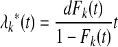
Cause-Specific Hazard: Definition and Estimator

The cause-specific hazard is formally defined as

A1

The cumulative cause-specific hazard is analogously

A2

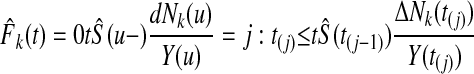
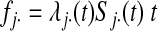
To estimate the cause-specific hazard, let

A3

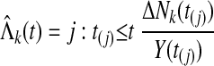
be the ordered event times, N_k(s) denote the number of failures of type k recorded at or before time s, and Y(s) the number of individuals at risk at time s. The nonparametric instantaneous hazard estimator for failure type k at time s is

A4

where

A5

For estimation purposes,

A6

and the cumulative hazard estimator (Nelson W. Technometrics 19:945-966, 1972; Aalen O. Scand J Stat 3:15-27, 1976) is

A7

The maximum likelihood estimator for the average hazard rate (or incidence density) is

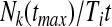A8

It can be thought of as an estimator for the time weighted average over (0, t) of the event rate for failure cause k, defined (Gardiner JC. Scand J Stat 9:31-36, 1982) by

A9

Cumulative Incidence Function: Definition and Estimator

The cumulative incidence function is defined as

A10

A nonparametric estimator for cause k, using the Kaplan-Meier estimator (Kaplan EL, Meier P. J Am Stat Assoc 53:457-481, 1958) for S(u), is

A11

Log-Rank Test

For patients in one of two groups A and B, a 2 × 2 table is formed for each unique time where one or more failures occurred (in either group). We denote the counts of the numbers of events by D_jm and number of individuals at risk by Y_jm for group A (j = 1) and B (j = 2), 3 so that at failure time t_m, the data are summarized as in Appendix Table A1, online only.

From the table, the expected number of failures in Group A (D_1m) under the null hypothesis of no difference in failure rate between groups is E_1m = D_m(Y_1m/Y_m). The sum over all M such tables of

A12

where

A13

gives the two-sample log-rank statistic, which has an asymptotic standard normal distribution (Mantel N. Cancer Chemother Rep 50:163 to 170, 1966). This and several other commonly used tests are described in a more general form by inclusion of a weighting factor that applies to each failure event (Gehan EA. Biometrika 52:203-223, 1965; Tarone RE, Ware J. Biometrika 64:156-160, 1977). Tests to simultaneously compare cause-specific hazard rates from k competing causes of failure among multiple groups have also been proposed (Kulathinal SB, Gasbarra D. Scand J Stat 8:147-161, 2002). This approach provides for specific hypotheses involving relationships among the cause-specific hazards to be tested, and contains the log-rank test as a special case when no competing risks are present.

Gray's Test

Gray (Gray RJ. Ann Stat 16:1141-1154, 1988) proposed a log-rank type of test that compares subdistribution hazards between groups, computing a weighted sum of differences in nonparametric estimates of the sub-distribution hazards

A14

between L groups. For the two-group case,

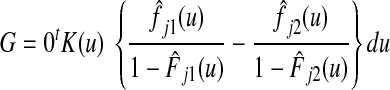A15

where

A16

and K(u) is a weight function. The quantity G divided by an appropriate variance estimate forms the standard normal test statistic.

Simulations and Data Examples

Simulations were executed using the R statistical language (http://www.R-project.org using a package “cmprsk” contributed by Robert Gray). Data examples were analyzed using R and the SAS statistical package to create the graphics. Although the log-rank test is included in essentially all commercial statistical analysis packages, Gray's test and the cumulative incidence function calculations are not as widely available, but numerous user-written modules exist. The recent book by Pintilie (Pintilie M. Competing Risks: A Practical Perspective. New York, NY, Wiley 2006) provides extensive computer code for competing risks analysis. We would be happy to provide our computer code on request.

Table A1.

Log-Rank Failure Table

Failure Resulting From Cause k?	Group A	Group B	Total
Yes	D1m	D2m	Dm
No	Y1m –D1m	Y2m –D2m	Ym –Dm
Total	Y1m	Y2m	Ym

NOTE. For group A, j = 1; for group B, j = 2.

Abbreviations: D_jm, counts of the numbers of events; Y_jm, number of individuals at risk.

REFERENCES

- 1.Peterson AV: Bounds for a joint distribution function with fixed sub-distribution functions: Applications to competing risks. Proc Natl Acad Sci U S A 73:11-13, 1976 [DOI] [PMC free article] [PubMed] [Google Scholar]
- 2.Gail MH: A review and critique of some models used in competing risk analysis. Biometrics 31:209-222, 1975 [PubMed] [Google Scholar]
- 3.Tsiatis AA: A nonidentifiability aspect of the problem of competing risks. Proc Natl Acad Sci U S A 72:20-22, 1975 [DOI] [PMC free article] [PubMed] [Google Scholar]
- 4.Gelman R, Gelber R, Henderson IC, et al: Improved methodology for analyzing local and distant recurrence. J Clin Oncol 8:548-555, 1990 [DOI] [PubMed] [Google Scholar]
- 5.Gaynor JJ, Feuer EJ, Tan CC, et al: On the use of cause-specific failure and conditional failure probabilities: Examples from clinical oncology data. J Am Stat Assoc 88:400-409, 1993 [Google Scholar]
- 6.Caplan RJ, Pajak TF, Cox JD: Analysis of the probability and risk of cause-specific failure. Int J Radiat Oncol Biol Phys 29:1183-1186, 1994 [DOI] [PubMed] [Google Scholar]
- 7.Gooley TA, Leisenring W, Crowley J, et al: Estimation of failure probabilities in the presence of competing risks: New representations of old estimators. Stat Med 18:695-706, 1999 [DOI] [PubMed] [Google Scholar]
- 8.Korn EL, Dorey FJ: Applications of crude incidence curves. Stat Med 11:813-829, 1992 [DOI] [PubMed] [Google Scholar]
- 9.Pepe MS, Mori M: Kaplan-Meier, marginal, or conditional probability curves in summarizing competing risks failure time data? Stat Med 12:737-751, 1993 [DOI] [PubMed] [Google Scholar]
- 10.Satagopan JM, Ben-Porat L, Berwick M, et al: A note on competing risks in survival data analysis. Br J Cancer 91:1229-1235, 2004 [DOI] [PMC free article] [PubMed] [Google Scholar]
- 11.Mantel N: Evaluation of survival data and two rank order statistics in its consideration. Cancer Chemother Rep 50:163-170, 1966 [PubMed] [Google Scholar]
- 12.Beltangady MS, Frankowski RF: Effect of unequal censoring on the size and power of the logrank and Wilcoxon types of tests for survival data. Stat Med 8:937-945, 1989 [DOI] [PubMed] [Google Scholar]
- 13.Lin DY: Nonparametric inference for cumulative incidence functions in competing risks studies. Stat Med 16:901-910, 1997 [DOI] [PubMed] [Google Scholar]
- 14.Gray RJ: A class of K-sample tests for comparing the cumulative incidence of a competing risk. Ann Stat 16:1141-1154, 1988 [Google Scholar]
- 15.Fine JP, Gray RJ: A proportional hazards model for the subdistribution of a competing risk. J Am Stat Assoc 94:496-509, 1999 [Google Scholar]
- 16.Fisher B, Costantino J, Redmond C, et al: A randomized clinical trial evaluating tamoxifen in the treatment of patients with node-negative breast cancer who have estrogen-receptor-positive tumors. N Engl J Med 320:479-484, 1989 [DOI] [PubMed] [Google Scholar]
- 17.Fisher B, Dignam J, Bryant J, et al: Five versus more than five years of tamoxifen therapy for breast cancer patients with negative lymph nodes and estrogen receptor-positive tumors. J Natl Cancer Inst 88:1529-1542, 1996 [DOI] [PubMed] [Google Scholar]
- 18.Prentice RL, Kalbfleisch JD, Peterson AV, et al: The analysis of failure times in the presence of competing risks. Biometrics 34:541-554, 1978 [PubMed] [Google Scholar]
- 19.Early Breast Cancer Trialists’ Collaborative Group: Tamoxifen for early breast cancer: An overview of the randomised trials. Lancet 351:1451-1467, 1998 [PubMed] [Google Scholar]
- 20.Chlebowski RT, Collyar DE, Somerfield MR, et al: American Society of Clinical Oncology technology assessment on breast cancer risk reduction strategies: Tamoxifen and raloxifene. J Clin Oncol 17:1939-1955, 1999 [DOI] [PubMed] [Google Scholar]
- 21.Freidlin B, Korn EL: Testing treatment effects in the presence of competing risks. Stat Med 24:1703-1712, 2005 [DOI] [PubMed] [Google Scholar]
- 22.Klein JP, Bajorunaite R: Inference in competing risks, in: Rao CR, Balakrishnan N (eds): Handbook of Statistics, Volume 23: Advances in Survival Analysis. Amsterdam, North-Holland, 2004, pp 291-312
- 23.Williamson PR, Kolamunnage-Dona R, Tudur Smith C: The influence of competing-risks setting on the choice of hypothesis test for treatment effect. Biostatistics 8:689-694, 2007 [DOI] [PubMed] [Google Scholar]
- 24.Pintilie M: Dealing with competing risks: Testing covariates and calculating sample size. Stat Med 21:3317-3324, 2002 [DOI] [PubMed] [Google Scholar]
- 25.Latouche A, Porcher R: Sample size calculations in the presence of competing risks. Stat Med 26:5370-5380, 2007 [DOI] [PubMed] [Google Scholar]
- 26.Kim HT: Cumulative incidence in competing risks data and competing risks regression analysis. Clin Cancer Res 13:559-565, 2007 [DOI] [PubMed] [Google Scholar]
- 27.Slud EV, Byar D: How dependent causes of death can make risk factors appear protective. Biometrics 44:265-269, 1988 [PubMed] [Google Scholar]
- 28.Di Serio C: The protective impact of a covariate on competing failures with an example from a bone marrow transplantation study. Lifetime Data Anal 3:99-122, 1997 [DOI] [PubMed] [Google Scholar]
- 29.Fine JP: Regression modeling of competing crude failure probabilities. Biostatistics 2:85-97, 2001 [DOI] [PubMed] [Google Scholar]
- 30.Klein JP, Andersen PK: Regression modeling of competing risks data based on pseudovalues of the cumulative incidence function. Biometrics 61:223-229, 2005 [DOI] [PubMed] [Google Scholar]
- 31.Jeong JH, Fine JP: Parametric regression on cumulative incidence function. Biostatistics 8:184-196, 2007 [DOI] [PubMed] [Google Scholar]
- 32.Smith RE, Bryant J, DeCillis A, et al: Acute myeloid leukemia and myelodysplastic syndrome after doxorubicin-cyclophosphamide adjuvant therapy for operable breast cancer: The National Surgical Adjuvant Breast and Bowel Project experience. J Clin Oncol 21:1195-1204, 2003 [DOI] [PubMed] [Google Scholar]
- 33.Benichou J, Gail MH: Estimates of absolute cause-specific risk in cohort studies. Biometrics 46:813-826, 1990 [PubMed] [Google Scholar]
- 34.Bentzen SM, Vaeth M, Pedersen DE, et al: Why actuarial estimates should be used in reporting late normal-tissue effects of cancer treatment. Int J Radiat Oncol Biol Phys 32:1531-1534, 1995 [DOI] [PubMed] [Google Scholar]
- 35.Chappell R: RE: Caplan et al: IJROBP 29:1183-1186; 1994, and Bentzen et al. IJROBP 32:1531-1534;1995. Int J Radiat Oncol Biol Phys 36:988-989, 1996 [DOI] [PubMed] [Google Scholar]