QUANTITATIVE PROTEOMICS OF THE ARCHAEON METHANOCOCCUS MARIPALUDIS VALIDATED BY MICROARRAY ANALYSIS AND REAL TIME PCR

SUMMARY

For the archaeon Methanococcus maripaludis, a fully sequenced and annotated model species of hydrogenotrophic methanogen, we report validation of quantitative protein level expression ratios on a proteome-wide basis. Using an approach based on quantitative multidimensional capillary HPLC and quadrupole ion trap mass spectrometry, coverage of gene expression approached that currently achievable with transcription microarrays. Comprehensive mass-spectrometry-based proteomics and spotted cDNA arrays were used to compare global protein and mRNA levels in a wild-type (S2) and mutant strain (S40) of M. maripaludis. Using linear regression with 652 expression ratios generated by both the proteomic and microarray methods, a product moment correlation coefficient of 0.24 was observed. The correlation improved to 0.61 if only genes showing significant expression changes were included. A novel two-stage method of outlier detection was employed for the protein measurements when Dixon’s Q-test by itself failed to give satisfactory results. The log₂ transformations of the number of peptides or isotopic peptide pairs associated with each ORF, divided by the predicted molecular weight, were found to have moderately positive correlations with two bioinformatic predictors of gene expression based on codon bias. We detected peptides derived from 939 proteins or 55% of the genome coding capacity. Of these, 60 were over-expressed and 34 were under-expressed in the mutant. Of the 1722 ORFs encoded in the genome, 1597 or 93% were probed by cDNA arrays. Of these, 50 were more highly expressed and 45 showed lower expression levels in the mutant relative to the wild-type. 15 ORFs were shown to be over-expressed by both methods and 2 ORFs were shown to be over-expressed by proteomics and under-expressed by microarray.

INTRODUCTION

The hydrogenotrophic methanogens are a major group of Archaea that conserve energy from the use of molecular hydrogen or formate to reduce carbon dioxide to methane. Methanococcus maripaludis is a model species of hydrogenotrophic methanogen, having favorable laboratory growth behavior, excellent genetic tools (1), and a fully sequenced genome (2). In another publication (3) we describe the molecular biology of a mutant of M. maripaludis (S40) in which the operon encoding the Ehb hydrogenase was disrupted and functional changes were observed that led to a model for the role of Ehb in energy metabolism. In the present paper we present validation of the multidimensional capillary HPLC/tandem mass spectrometry approach (aka MudPIT (4, 5)) to quantitative and qualitative proteomics for M. maripaludis by comparison with mRNA expression. Transcriptome analysis was performed in which the ehb mutant and wild-type strains were compared globally for all known genes under the same culture conditions as the proteomics. For a subset of genes the proteomic results were further validated by real time quantitative RT-PCR. The relative absence of evidence for posttranscriptional gene regulation and the favorable protein extraction properties of M. maripaludis were suggestive of the hypothesis that, under the experimental conditions reported here, the transcriptome and proteome should both be reasonably complete and show parallel trends for most genes. We also consider codon bias relationships as they relate to the proteomic results, a two-stage algorithm for outlier detection in proteomics, and some of the unique strengths and weaknesses of comprehensive expression ratio calculations based on direct measurement of protein using MudPIT technology. Our purpose in undertaking these studies was primarily to better understand where the MudPIT approach to global protein measurements fits in to the broader scheme of our armamentarium for doing systems biology with microbes. More specifically, we address the question is it reasonable to expect whole proteome level expression ratios from this approach to be comparable in terms of coverage and quantitative reliability to what can be achieved for the transcriptome using microarray technology?

MATERIALS AND METHODS

Methanococcus maripaludis strains S2 and S40, genome sequence for S2, and growth conditions for qualitative proteomics of S2

For information regarding the molecular genetics of the M. maripaludis strains used and the construction of the ehb mutant (S40), see Porat et al. (3). Details regarding the genome sequence and annotation of M. maripaludis strain S2 have been published (2). The most current annotations can be accessed at http://faculty.washington.edu/leighj/mmgenome/.html. Growth conditions for the five chemostat and batch cultures of S2 grown for purely qualitative proteomic analysis are described in the “growth conditions” note to electronic supplementary Table S3.

Differential ¹⁵N:¹⁴N-labeling of proteins

To prepare differentially ¹⁵N-labeled proteins, strains S2 and S40 were grown as described (6) in McNA medium (McN plus 10 mM sodium acetate) containing either 4.6 mM ¹⁵N ammonium sulfate (instead of ammonium chloride) or unlabeled ammonium sulfate in side-arm bottles. The bottles were constructed from 160 ml serum bottles by fusing a 28 ml culture tube to the side. Thus, it was possible to follow the culture absorbance in a spectrophotometer without removing samples from the cultures. Before use, glassware was immersed in 1 M HCl overnight, rinsed with water, autoclaved in water with soap, rinsed in deionized water, and dried. To remove O₂ adsorbed to the glassware, the bottles were stored in the anaerobic chamber at least a day before use. Stoppers were autoclaved for 20 min in 0.1 M NaOH, rinsed with deionized water, dried and stored in the anaerobic chamber at least a day before use. Four bottles each containing 10 ml of culture were prepared for each growth condition. Cultures were initially pressurized to 276 kPa with H₂/CO₂ gas (80:20 [vol/vol]) and repressurized twice daily. When the cultures reached an average OD₆₀₀ of 0.56, 40 ml of the S2 culture grown with ¹⁴N was mixed with 40 ml of the S40 culture grown with ¹⁵N to form sample 1. The reciprocal mixture, called sample 2, was also prepared with cultures of S2 grown with ¹⁵N and cultures of S40 grown with ¹⁴N. Because of its slower growth, the mutant was harvested after 21 h while S2 was harvested after 13 h. The cell mixtures were centrifuged at 10,000 × g for 30 min at 4°C. After resuspending the cells in 2 ml of buffer B (100 mM ammonium bicarbonate (pH 9.0) and 2 mM DTT), the cells were lysed by freezing at -20°C. The resuspended frozen cells were stored at -20°C. Upon thawing, 10 U of DNase I were added, and the suspension was incubated for 15 min at 37°C. After microscopic inspection to insure lysis the cell debris and the unbroken cells were pelleted by centrifugation at 8,000 × g for 30 min at 4°C. Supernatants and pellets (resuspended in 0.5 ml buffer B) were used separately for protein preparation as follows. Four protein samples were obtained from the two mixtures, two supernatants (CE1 and CE2) and two pellets (PT1 and PT2). For each sample, 200 μl of centrifuged cell lysate containing approximately 0.5 mg of total protein was brought to a final volume of 370 μl containing 40 μl DNAse/RNAse solution (1 mg/ml DNAse I, 500 μg/ml RNAse A), 0.15% RapiGest (Waters, Boston, MA), 5 mM DTT, and 50 mM Tris-HCl, at pH 8.0. The RapidGest is an acid labile bifunctional molecule designed to serve as a substitute for conventional detergents, that is less likely to interfere with the mass spectrometry. The samples were immediately placed in boiling water for 1.5 to 2.0 min until the solution ceased to show obvious viscosity due to residual DNA. Each sample was then transferred onto ice. The proteins were further reduced by the addition of 5 mM DTT at 37°C for 30 min and then alkylated with 10 mM iodoacetamide at 30°C for 30 min in the dark. Each sample was then adjusted to give a solution containing 50 mM NH₄HCO₃ and 5 mM CaCl₂. Trypsin, 15 μg of sequencing grade (Promega, Madison, WI), was added, and the mixture was incubated at 37°C for 4 hours. The sample was acidified with TFA to quench the digestion and concentrated to 200 μl using a vacuum centrifuge (RC10-22, Jouan Inc. Winchester, VA).

Liquid chromatography and tandem mass spectrometry

Off-line HPLC fractionation, 2D microcapillary HPLC, and LCQ ion trap mass spectrometry were essentially as described (7), with minor modifications. Samples were vortexed and centrifuged at 14,000 rpm in a microcentrifuge (Eppendorf 5415C) for 8 min to remove insoluble material. 30 μl of 50% acetonitrile was added, followed by another vortex and centrifugation at 14,000 rpm for 4-5 min to remove any remaining insoluble material. Samples were fractionated using a YMC-Pack™ PolymerC18™, S-6, 2.0 × 150 mm reversed-phase HPLC column (Waters, Milford, MA). The mobile phase was H₂O and acetonitrile with 0.1% TFA. Peptides were eluted with increasing acetonitrile (2% to 60% in 60 min) at 0.4 ml/min. For samples CE1 and CE2, eluant containing peptides was detected by UV absorption at 214 nm and was fed one ml at a time into each of five tubes successively, rotating through all five tubes several times until all peptide-containing eluant was collected, resulting in five combined fractions. For samples PT1 and PT2 only two combined fractions were similarly collected. Each combined fraction was concentrated to 100 μl using a vacuum microcentrifuge, and acetic acid was added to a final concentration of 0.5% (v/v). Approximately 2.5 μl from each combined fraction was analyzed using a 2D microcapillary HPLC system (7, 8) combined with a Thermo-Finnigan LCQ Classic or LTQ mass spectrometer in a semi-automated, data-dependent manner as previously described (7). Data acquired for the qualitative analysis of unlabeled strain S2 using the LTQ linear ion trap were similar and differed mainly in the number of usable mass spectra acquired per unit time. In our hands the LTQ could collect data about 3 to 5X faster, consistent with the experience of other laboratories (9).

Proteomic data collection and analysis

Raw mass spectral data were collected, consisting of full scan (MS¹) data and, for selected parent ions, CID scan (MS²) data. The SEQUEST algorithm (10) was used to identify MS² spectra that were candidates for peptides encoded in the M. maripaludis strain S2 ORF database (2), (GenBank Accession BX950229). Our Mmp (Methanococcus maripaludis) FASTA database (version dated January 21, 2005) was enlarged by adding approximately 25% of the nrdb human subset in order to increase the size of the database to about 21 Mbytes in order to avoid statistical problems associated with searching very small databases. Two separate SEQUEST parameter files, one for ¹⁴N-peptides and one for ¹⁵N-peptides, were used (4, 5, 10). DTASelect (11) was then used to filter the results based on the following criteria: peptides were required to be fully tryptic (beginning and ending at adjacent predicted trypsin digestion sites); the minimum peptide length was four amino acids; ΔCn/Xcorr values for different peptide charge states were 0.08/1.9 for +1, 0.08/2.0 for + 2, and 0.08/3.3 for +3. This process generated two DTASelect-filter.txt files, one for ¹⁴N-peptides and one for ¹⁵N-peptides.

A program calculating the protein expression ratios for S40:S2 was written under the File-Maker 7.0 environment.² Briefly, peptide pairs were found for each identified peptide that was a unique peptide (sequence present in only one predicted ORF in the mmp database) in both DTASelect-filter.txt files as follows: For the parent ion selected for each CID scan, the m/z value for the corresponding isotopic “flip” ion was calculated. The raw MS¹ data was then searched for an ion with that m/z value in the full scan from which the original CID scan was derived during the parent ion selection process. If no “flip” ion was found, then the noise value near the predicted m/z for the flip ion was used instead. A non-zero value for the missing member of the ¹⁵N/¹⁴N peptide pair was essential in order to avoid prematurely rejecting data for potentially highly regulated genes. The raw data were then similarly searched for “heavy” and “light” peptide pairs in the MS¹ scans immediately prior to and immediately after the scan used to select the original parent ion. Of the three MS¹ scans, data were retained for the scan with the highest signal intensity. This process was repeated for as many “heavy” ¹⁵N and “light” ¹⁴N peptide pairs as the program could find for each ORF.

An average ratio was calculated for each protein from all the ¹⁵N:¹⁴N and ¹⁴N:¹⁵N peptide pairs associated with that protein. Normalization of the average ratios was done in a manner similar to methods that are employed for microarrays (12). Briefly, a frequency distribution histogram of the log₂ transformed ratios was constructed (data not shown), then the ratios were normalized by a factor which made the distribution center at 0 (12). The number of peptide pairs collected per ORF (n₁) was used as a measure of reliability and analytical precision. Differential protein levels were regarded as significant if n₁ was equal to or greater than three and the ratio (S40:S2) ± the standard deviation was above or below 1.0. These calculations were done separately for each of the four samples, CE1, CE2, PT1 and PT2. Finally, data from all four samples were combined, and used to make a composite analysis (summary) of the expression pattern for S40:S2 (see supplementary Table S2). For the composite analysis, peptide ratios determined to be outliers were eliminated. The detection of outliers was done in two steps for each list of peptide ratios associated with an ORF. For the first stage, Dixon’s Q-test (13) was used, in the second stage, a MAD (median of the absolute deviation) modified z-score test (14, 15, 16) with a cutoff value of 3.5 was used.

Confirmation by peptide synthesis

The following five peptides were synthesized commercially (Anaspec, San Jose, CA) and used for comparison of the original CID mass spectrum (MS²) with the CID spectrum acquired for the synthetic peptide standard. The Mmp number is given for each ORF followed by the sequence tag: Mmp0512, ELQKYAK; Mmp0512, NACKMGAAKFR; Mmp1456, IGQIPFR; Mmp1517, HFGAWSEFR; Mmp1517, AWYEGLALAIFLK.

Preparation of RNA

Cells were grown as for the differential ¹⁵N:¹⁴N-labeling of proteins except that only ¹⁴N was used. When the average OD₆₀₀ reached 0.55, the cultures were rapidly cooled in an ice water bath. For these experiments, cultures of S2 and S40 reached this optical density after 12 and 36 h, respectively. The cells were collected by centrifugation at 8,000 × g for 30 min at 4°C, washed in 1 ml Mc buffer (McN medium (6) without sodium bicarbonate) and stored at -70°C. The cells were then resuspended in 200 μl of minimal nitrogen-free growth medium (excluding sulfide (17)) and lysed by the addition of 250 μl of RLT buffer (Qiagen, Valencia, CA). 350 μl of 100% ethanol (Aaper, Shelbyville, KY) were then added and the RNA purified on RNeasy columns (Qiagen). Aliquots of RNA were then treated with DNase using DNA-Free (Ambion, Austin, TX). Reactions contained 0.4 units of DNAse I/μl of reaction mixture and were terminated with 10 μl of DNAse inactivation reagent (Ambion).

The quality of the RNA samples was checked using an Agilent 2100 Bioanalyzer (Agilent Technologies Inc, Palo Alto, CA). The absence of DNA was confirmed by a PCR reaction using a Biometra T gradient thermocycler (Whatman Biometra, Goettingen Germany) and primers QRNAr and QRNAf (supplemental Table S1) for ORF Mmp0608.

Array Labeling and Hybridization

Arrays constructed by generating PCR products of approximately 500 base pairs in length for each of the predicted ORFs were purchased from Integrated Genomics (Chicago, IL) and spotted in duplicate on mirrored slides at the University of Washington Center for Expression Arrays. Labeling reactions were conducted with the amino allyl cDNA labeling kit (Ambion) using a modification of the published procedure. For each reaction, 5-10 μg of RNA and 4 μg of random decamers (IDT, Coralville, IA) were incubated at 75°C for 7 minutes, then briefly centrifuged at room temperature. First-strand cDNA synthesis was carried out in 1× RT buffer, 10 units RNAse inhibitor, 0.5 mM dATP, 0.5 mM dCTP, 0.5 mM dGTP, 0.15 mM dTTP, 0.15 mM amino allyl dUTP, and 400 units reverse transcriptase for 10 min at room temperature, followed by 2 h at 42°C. The RNA template was then hydrolyzed by adding 4 μl of 1 M NaOH and incubating at 65°C for 15 minutes. The reaction was neutralized by the addition of 10 μl of 1 M HEPES; cDNA was precipitated by the addition of 3.4 μl of 3 M sodium acetate, 1 μl of 5 mg/ml glycogen, and 100 μl of 100% ethanol (Aaper, Shelbyville, KY), incubation for 15 min at −20°C, and centrifugation at maximum speed in a microcentrifuge for 30 min at 4°C. The samples were then washed with 75% ethanol, and the supernatants were discarded. For NHS-Cy dye coupling, the samples were resuspended in 4.5 μl of coupling buffer (Ambion), 2.5 μl RNAse free H₂O (Ambion), and 3 μl of either NHS-Cy3 or NHS-Cy5 (Amer-sham-Pharmacia, Piscataway, NJ) and incubated at room temperature in the dark for 1 hour. The reaction was quenched with the addition of 6 μl of 4 M hydroxylamine (Ambion) followed by a 15 min incubation at room temperature in the dark. Unincorporated dye was removed by adding 100 μl of PB buffer (Qiagen) and 750 μl of 100% ethanol (Aaper), and applying the sample to a Minelute reaction clean-up column (Qiagen). Samples were eluted from the column with 60 l of RNAse free H₂O (Ambion). The whole, undiluted sample was analyzed using a spectrophotometer to determine DNA yields and dye concentrations. Only samples with at least 35 pmol of dye per mg DNA were employed for hybridization.

Samples were prepared for hybridization by mixing 100-120 pmol each of the Cy3 and Cy5-labeled cDNA and taking them to dryness in a Speed-Vac (Jouan, Winchester, VA). The samples were then resuspended in 60 l of hybridization buffer (Agilent, Palo Alto, CA), boiled for 3 minutes, and incubated on ice for 30 seconds.

Slides were washed in sterilized dH₂O and dried with pressurized nitrogen gas. Resuspended samples were then applied along one edge of the slide, and a clean glass 24×60 mm cover slip (VWR, West Chester, PA) was lowered slowly over the sample starting with that edge. The slides were then sealed in a plastic container with reservoirs of dH₂O to maintain humidity, and the hybridization carried out at 42°C for 14-16 hours in the dark.

All post-hybridization washes were performed in 50 ml conical tubes (Greiner, Longwood, FL). A brief wash in 1× SSC + 0.2% SDS was used to remove the cover slip, followed by a 10 min wash in 1× SSC + 0.2% SDS and two 10 min washes in 0.1× SSC + 0.2% SDS, all at 54°C, with rotation in a hybridization oven covered with aluminum foil. Finally, slides were subjected to two one min washes at room temperature in 0.1× SSC, rinsed briefly with dH₂O, and dried with pressurized nitrogen gas.

Array data collection and analysis

Slides were scanned at the University of Washington Center for Expression Arrays on a Molecular Dynamics Gen III array scanner. Images were collected separately for each duplicate half of the slide. Images taken for the Cy3 and Cy5 channels were stored as paired gel files. Spots were identified, and the local background was subtracted using the SpotFinder software from TIGR.³ Four biological replicates were analyzed, each with duplicate arrays on each slide and with flip-dye hybridizations, making a total of sixteen measurements for each gene. Data were Loess-normalized using the S+ array analyzer (Insightful, Seattle, WA). Average expression ratios and unadjusted p values were calculated for each gene across all replicates using the S+ array analyzer, employing a Wilcoxon non-parametric significance test for the p value calculations (18). Genes with p values less than 0.01 were regarded as differentially expressed.

Real time RT-PCR

RNA was purified as described above. Real time RT-PCR was performed on a RotorGene 2000 instrument from Corbett Research (Westborough MA). Software version 4.6 was used during the run, and data were analyzed on software version 6.0. Real time RT-PCR was carried out using SuperScriptIII Platinum One-Step Quantitative real time RT-PCR system by Invitrogen (Carlsbad, CA) according to the manufacturer’s protocol. Primer and TaqMan probe concentrations were 200 nM, MgSO₄ was adjusted to 3.5 mM, and RNA was added to 50 ng per 20 μl reaction. Cycling parameters consisted of the RT reaction at 55°C for 35 min, initial denaturation at 95°C for 2 min, and 35 cycles of 95°C for 15 sec and 60°C for 30 sec. All samples were performed in triplicate with appropriate controls (no template control and no amplification control). 16S rRNA was used as a standard (details of TaqMan probes in supplemental Table S1).

Bioinformatics

The quantitative combined array/proteomics dataset (supplement Table S2), the qualitative proteomics dataset (supplement Table S3), color images of the M. maripaludis proteome and transcriptome (Fig. 2), the signal intensity/peptide number calculations (Fig. 4), and the codon bias calculations (Fig. 5) were generated using a Filemaker Pro 7.0 application developed in-house (Filemaker, Inc., Santa Clara, CA).²

Fig. 2. Genomic representation of the proteome (A) and transcriptome (B).

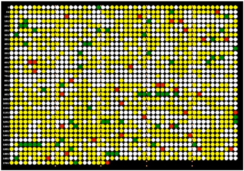
Each circle represents an ORF in the order it is encoded in the genome (Mmp0001 in upper left, Mmp1722 at end of bottom row). Colored circles indicate results for combined proteome analyses of the sum of four samples (CE1, CE2, PT1, PT2) and for array analyses. Green=up in S40 mutant, red=down in S40 mutant, yellow=data collected but no statistical evidence for differential expression, white=no data because mRNA not probed or protein not detected. Note that the meaning of yellow and white is somewhat different for the proteome and the transcriptome. Because absolute detection is measured in the proteome, yellow circles in Fig. 2A indicate that the protein was present, while white circles indicate that no protein was detected at our limit of detection for qualitative identification (an interpretable MS² daughter ion spectrum was not observed at a signal intensity threshold of 40,000 data system counts for the parent ion when using the LCQ ion trap mass spectrometer). In contrast, yellow in Fig. 2B indicates only that a probe was included in the array, and white that a probe was not included.

Fig. 4. Scatter plots illustrating relationships among total signal intensity, the number of heavy/light peptide pairs recovered per ORF (n₁), the number of redundant peptides recovered per ORF (n₂), and the relative standard deviations for the protein level expression ratios (S40:S2) calculated for each ORF.

A, correlation of the number of redundant peptides (n₂) observed for each protein with the number of peptide pairs (n₁) for the same protein. Observations from 939 proteins (see supplement, Tables S2 and S3) were used to generate the plot. B, correlation of total signal intensity observed for all peptide “hits” associated with a given ORF and the number of observed redundant peptides (n₂). C, relative standard deviation (RSD) of the mean expression ratio for 688 proteins (n₁≥3). The average RSD is 44%, which is driven largely by the data points in the upper left. Many of the data points with larger RSD values share a common characteristic, a non-detect in either the numerator or the denominator, e.g. instances in which a strong signal was observed for one condition but only baseline noise or a weak signal was observed for the corresponding peptide in the other condition, see discussion. At high values of n₁ the RSD converges to about 35%. D, distribution of the 688 average protein expression ratios (n₁≥3) as a function of n₁. The 15 data points marked in green are the genes that are considered as up-regulated in S40 with respect to S2, as determined by both cDNA microarrays and proteomics. The two red data points are the genes that show down-regulation by array but up-regulation by proteomics, see supplement Table S2 for a complete summary of the quantitative dataset. The 15 genes for which there was a consensus for up-regulation yielded mean protein expression ratios ≥2. Statistically and biologically significant expression changes stand out more clearly as n₁ and n₂ go to higher values, see text.

Fig. 5. Correlation between gene expression level predicted by codon usage bias and identified peptide numbers per ORF normalized by protein molecular weight.

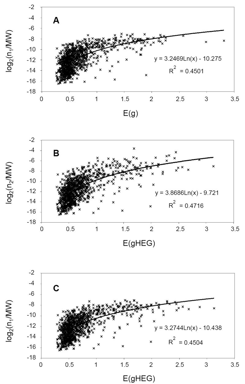
E(g) and E(gHEG) are Karlin’s measures of predicted gene expression calculated for each gene (g) based on codon usage bias (20). A, E(g) = B(g|G) / {0.5B(g|RP) + 0.25B(g|Tf) + 0.25B(g|MR)} and is based on the data for ribosomal proteins (RP), transcription elongation factors (Tf), and methyl-coenzyme M reductase subunits (MR) listed in supplemental Table S2. B and C, E(gHEG) = B(g|G) / B(g|HEG) and is based on highly expressed genes (HEG) chosen by the criterion n₂ > 300 (supplemental Table S2). n₁ = number of peptide pairs and n₂ = number of redundant peptides shown for each entry in supplemental Table S2. MW = predicted molecular weight.

RESULTS

Summary statistics for the Methanococcus maripaludis proteome and transcriptome

We measured relative gene expression at the proteome and transcriptome levels in the mutant S40 compared to the wild-type S2. Proteomic data were based on mass spectrometric identification and quantitation of peptide pairs as described in Materials and Methods. Each peptide pair consisted of a unique amino acid sequence (present in only one predicted Mmp protein) either labeled metabolically with ¹⁵N (>98% incorporation) or ¹⁴N at natural abundance. Fig. 1 summarizes the observed expression changes for the entire organism. Table 1 describes expression changes that were observed for specific genes of interest believed to play a role in energy metabolism. Table 2 describes other Mmp genes that showed statistically significant expression changes between strains S2 and S40. Proteins encoded by 939 of the 1722 ORFs were detected, representing 55% of the coding capacity of the genome. Of these, 60 were up-regulated in the S40 mutant relative to the wild-type, 34 were down-regulated, and the remainder lacked statistical support for regulation. Our spotted arrays contained DNA corresponding to 1597 of the 1722 ORFs encoded in the genome. Of these, 50 were up-regulated in the S40 mutant relative to the wild- type, 45 were down-regulated, and the remainder lacked statistical support for regulation. Both mRNA and protein data were recorded for 889 ORFs (probed in arrays and detected in the proteome). Agreement occurred where 15 ORFs were up-regulated by both methods, and 744 had no evidence of regulation by either method. The results from the two approaches to global gene expression differed where 56 ORFs were regulated only in the arrays (24 up and 32 down), 72 were regulated only in the proteome (41 up and 31 down), and two were down-regulated in the arrays but up-regulated in the proteome. The complete quantitative datasets for both mRNA and protein level expression ratios, including the statistics used to assign significance with respect to expression changes, are summarized in the supplement (Table S2).

Fig. 1. Combined summary of proteome and transcriptome for S40 over S2 expression ratios.

Numbers of ORFs in each category are shown. Up=significantly higher expression in S40 compared to S2. Down=significantly lower expression in S40 compared to S2. No change=no significant difference. NP=not probed in arrays. ND=not detected in proteomics. Totals are given: first row contains total numbers of ORFs up, down, not changed, and not probed in the transcriptome; first column contains total numbers of ORFs up, down, not changed, and not detected in proteome. The total number of ORFs in the annotated genome is 1722 (2). The complete listing of expression ratios is given in supplementary Table S2.

Table 1.

Expression of genes involved in energy conversion by proteomic and transcriptional array analyses

ORF/Function	Descriptiona	Proteomic datab			Array datac
		Avg Ratio	n1	Std dev	Ratio	std dev	p value
A1A0-ATPase
Mmp1038e	subunit H	0.96	42	0.25
Mmp1039	subunit I	1.09	85	0.33	0.65	0.14	3.43E-04
Mmp1041	subunit IE	1.17	38	0.41	0.65	0.18	7.96E-04
Mmp1040d	subunit K				0.69	0.24	1.76E-02
Mmp1042	subunit C	1.13	92	0.40	0.63	0.15	1.41E-04
Mmp1043e	subunit F	1.25	39	0.39
Mmp1044	subunit A	1.20	150	0.38	0.75	0.17	1.16E-02
Mmp1045	subunit B	1.11	103	0.39	0.74	0.13	1.04E-03
Mmp1046	subunit D	1.30	55	0.56	0.71	0.11	2.00E-03
Methyl-coenzyme M reductase I
Mmp1555	beta subunit	1.09	209	0.46	0.67	0.10	2.57E-03
Mmp1556	protein D	0.96	19	0.57	0.72	0.20	9.64E-01
Mmp1557	protein C	1.31	6	0.93	0.76	0.27	1.31E-01
Mmp1558	gamma subunit	1.01	194	0.33	0.74	0.12	2.57E-03
Mmp1559	alpha subunit	0.98	188	0.35	0.81	0.08	4.70E-03
N5-methyltetrahydromethanopterin:coenzyme M methyltransferase
Mmp1560	subunit E	1.28	8	0.60	0.65	0.18	7.96E-04
Mmp1561d	subunit D				0.66	0.14	6.66E-03
Mmp1562	subunit C	0.92	6	0.32	0.90	0.40	1.42E-01
Mmp1563	subunit B	1.22	44	0.37	0.71	0.15	3.43E-04
Mmp1564	subunit A	1.43	17	0.29	0.70	0.18	8.33E-03
Mmp1565e	subunit A and F related proteins	0.93	29	0.33
Mmp1566d	subunit G				0.71	0.14	2.62E-02
Mmp1567	subunit H	1.11	109	0.42	0.73	0.17	5.29E-03
Flagella
Mmp1666	flagellin B1 percursor	0.97	3	0.47	0.34	0.15	5.51E-05
Mmp1667d	flagellin B2				0.31	0.11	1.41E-06
Mmp1668	flagellin B3	0.99	22	0.40	0.36	0.16	3.56E-06
Mmp1669	flagella accessory protein C	1.04	2	0.24	0.39	0.16	1.70E-06
Mmp1670	flagella accessory protein D	1.02	35	0.19	0.55	0.17	1.64E-04
Mmp1671	flagella accessory protein E	1.09	20	0.45	0.65	0.14	2.37E-02
Mmp1672d	flagella accessory protein F				0.63	0.12	2.97E-04
Mmp1673	flagella accessory protein G	1.14	1	-	0.75	0.10	4.18E-02
Mmp1674d	flagella accessory protein H				0.77	0.20	1.87E-01
Mmp1675	flagella accessory protein I	1.34	5	1.55	0.85	0.12	1.32E-01
Mmp1676	flagella accessory protein J	2.40	3	3.23	0.89	0.09	2.74E-01

^aThe ORF description is derived from the genome annotation (2).

^bNumerical data for proteomic analysis report average S40:S2 ratios, numbers of peptides pairs (n₁) used to derive ratios, and standard deviations, for the combination of four samples as described in the text and supplementary Table S2. Bold indicates significantly higher expression in the mutant, bold italics lower expression.

^cNumerical data for array analysis report average S40:S2 ratios, standard deviations, and p values (less than or equal to 0.01 was taken to indicate differential expression). Number of replicates for array analysis was 16.

^dProtein not detected.

^emRNA not probed.

Table 2.

Expression of other potentially regulated genes by proteomic and transcriptional array analyses^a

ORF/Function	Description	Proteomic data			Array data
		Avg Ratio	n1	Std dev	Ratio	std dev	p value
Transport /regulation
Mmp0165	ABC transporter, family 2	1.49	2	0.93	1.77	0.67	5.94E-03
Mmp0166	integral membrane protein	1.41	6	1.14	2.86	1.75	3.39E-05
Mmp0167	ABC transporter ATP binding protein	1.30	62	0.73	4.46	2.46	5.11E-06
Mmp0168	transcriptional regulator PadR-like	0.99	16	0.23	3.32	1.71	7.29E-06
Mmp1510	amidotransferase subunit A	0.90	15	0.45	1.29	0.13	3.28E-03
Mmp1511	sodium:alanine symporter	2.31	18	1.07	1.39	0.22	7.45E-03
Mmp1512b	alanine racemase				1.00	0.10	9.40E-01
Mmp1513	alanine dehydrogenase	1.03	19	0.42	0.93	0.10	3.86E-01
Translation
Mmp1319	SSU ribosomal protein S13	1.06	22	0.74	1.25	0.17	1.75E-01
Mmp1320	SSU ribosomal protein S4P (S9E)	1.13	71	0.40	1.49	0.49	7.04E-02
Mmp1321	SSU ribosomal protein S11	1.04	41	0.29	1.57	0.29	2.57E-03
Mmp1322	RNA polymerase, alpha chain	1.18	18	0.46	1.52	0.22	9.11E-04
Mmp1323	ribosomal protein L15	1.04	24	0.36	1.56	0.26	1.55E-03
Mmp1324	ribosomal protein L13	1.14	32	0.57	1.53	0.21	9.31E-03
Mmp1325	SSU ribosomal protein S9P	0.98	46	0.30	1.86	0.32	2.05E-05
Hypothetical proteins
Mmp0883	hypothetical protein	0.65	4	0.01	0.79	0.15	5.46E-02
Mmp0884	hypothetical protein	0.84	7	0.14	0.87	0.27	5.22E-01
Mmp1158	conserved hypothetical protein	1.15	8	0.67	0.62	0.11	1.04E-04
Mmp1159	ferritin	0.77	4	0.58	0.69	0.16	1.29E-02
Mmp1160b	conserved hypothetical protein				0.65	0.12	6.94E-04
Mmp1161	conserved hypothetical archaeal protein	1.70	20	0.92	0.61	0.15	6.94E-04
Mmp1162	flavodoxin:beta-lactamase-like protein	1.14	19	0.39	0.74	0.18	1.32E-01
Mmp1163b	CutA1 divalent ion tolerance-related protein				0.71	0.13	9.31E-03
Mmp1212	undefined product	1.03	54	0.29	0.65	0.16	1.19E-03
Mmp1213	undefined product	1.08	30	0.49	0.70	0.16	9.31E-03
Mmp1714	conserved hypothetical protein	1.82	3	1.17	0.62	0.15	1.36E-03
Mmp1715	putative GTPase methylenetetrahydromethanopterin	1.68	3	0.48	0.57	0.14	2.43E-05
Mmp1716	dehydrogenase-related protein	1.23	15	0.36	0.57	0.12	3.99E-05

^aData specifications as in Table 1. See supplementary Table S2 for the complete list of results for all genes.

^bProtein not detected.

Corroboration of quantitative results

The results showing differential expression in the proteome and transcriptome were corroborated in several ways. First, as mentioned above 15 ORFs showed similar regulation in the proteome and transcriptome, all in the up-direction in the mutant. Second, in many cases the regulatory pattern was further supported by the observation that the ORFs were components of multicistronic operons in which most of the genes showed the same trends.

This pattern is apparent in Fig. 2, where colored images of the proteome (Fig. 2A) and transcriptome (Fig. 2B) present the ORFs by Mmp number, following the physical map of the genome (2). In these plots green indicates statistically supported higher expression in the mutant compared to wild-type, red indicates lower expression, yellow indicates no statistical support for differential expression, and white indicates no data for the reasons described in the figure legend. For the sake of simplicity and because the errors associated with the expression ratios are sufficiently large in both the proteome and the transcriptome, we indicate only the direction of change in green and red, not the magnitude of change. This operon-based corroboration was nearly always found in those 15 cases where both the arrays and the proteome showed similar regulation. It was frequently the case also where only the arrays showed regulation: of the 56 ORFs that were regulated in the array only, 29 were in one of eight multicistronic operons with other ORFs that were coregulated. Similarly, for the 72 ORFs regulated only in the proteome, 13 ORFs were in one of six operons that were coregulated. Hence, there were good reasons to believe that many of the differences in expression observed by only one method were biologically significant. Third, the results from the proteome and the transcriptome were positively correlated overall. This relationship is shown in Fig. 3, where the expression ratios are plotted for the proteome vs. the transcriptome for 652 ORFs that passed quantitative quality control criteria for both protein and mRNA measurements in both the mutant and the wild-type strain. Certain ORFs that were probed for but that did not yield signals associated with significant hybridization in the arrays were eliminated from the data used to plot Fig. 3, as were nondetects at the protein level.

Fig. 3. Scatter plot showing the correlation of mRNA and protein expression.

The plot of log₂ transformed differential mRNA and protein expression ratios (30) was generated using the proteomic data that contained ≥3 unique peptides for each ORF. Among a total of 652 ORFs for which both protein and mRNA data were recorded, 15 appeared to be up-regulated in the S40 mutant by both methods (shown in green); two ORFs showed statistically significant opposite trends in regulation between mRNA and protein levels and are marked as foreground in green for protein level (up-regulation) and background in red for mRNA levels (down-regulation). All other data points are in black. Product-moment correlation coefficients (18) were: 0.24 for all 652 data points; 0.54 for 121 genes with microarray p values < 0.05; 0.61 for 61 genes with p values < 0.01; and 0.61 for the 17 data points (shown in color) that showed significant changes in both mRNA and protein levels.

Although the product moment correlation coefficient was weak at 0.24, one must keep in mind that these ORFs included most of those for which both proteomic and transcriptomic data were acquired, regardless of standard deviation or p value, implying mostly random noise centered about a net expression change of zero. If only genes showing microarray p values of less than 0.01 were included, the correlation improved to 0.61, see Fig. 3. Finally, the results from proteomics and transcriptome arrays agreed with enzyme activity measurements and real time RT-PCR. Enzymatic assays of pyruvate oxidoreductase (POR) activity showed that S40 contained 2.6 ± 0.9 times the activity found in S2 (3). This value is very close to the average of the expression ratios determined for the ORFs in the operon encoding the POR subunits (Mmp1502-1507), by both proteomics (2.6 ± 0.3) and arrays (2.5 ± 0.4). Furthermore, a comparison of real time RT PCR, transcriptome array, and proteomics results for seven selected ORFs is presented in Table 3. ORFs were selected to represent different patterns of regulation in the transcriptome and the proteome. Real-time RT-PCR and transcriptome arrays agreed in all cases, within their ranges of precision. Real-time RT-PCR and proteomics agreed in all cases except one, and conflicted in the case of ORF Mmp1478.

Table 3.

Comparison of real time RT PCR, array and proteomics results for selected genes

Gene Name	Mmp Number	PCR Ratioa	Array Ratiob	P valuec	Proteomic Ratiod	n1e
16S RNAf	RNA standard	0.999 +/- 0.002
ppsA	Mmp1094	1.0 +/- 0.5	1.00 +/- 0.09	0.73	1.2 +/- 0.5	157
cbiA	Mmp1478	1.0 +/- 0.1g	1.02 +/- 0.07	0.65	1.5 +/- 0.2	10
atpB	Mmp1045	0.8 +/- 0.0	0.7 +/- 0.1	1.0 × 10-3	1.1 +/- 0.4	103
mtrE	Mmp1560	0.9 +/- 0.3g	0.6 +/- 0.2	8.0 × 10-4	1.3 +/- 0.6	8
mtrA	Mmp1564	0.9 +/- 0.2	0.7 +/- 0.2	8.3 × 10-3	1.4 +/- 0.3	17
porEh	Mmp1503	4.4 +/- 2.1g	2.8 +/- 0.6	1.5 × 10-5	2.0 +/- 0.9	29
ehbL	Mmp1623	4.9 +/- 0.2	4.4+/- 0.8	1.0 × 10-6	3.5 +/- 2.1	17

^aExcept as noted, real time RT PCR assays were done in triplicate from a single RNA sample and normalized to 16S rRNA as an unregulated standard.

^bArray ratios were calculated from four biological replicates, each with flipped dye slides containing two copies of the array. See supplementary Table S2 for the complete listing.

^cP values were calculated using a Wilcoxon nonparametric significance test (18) and represent the probability that the null hypothesis (a ratio of 1 indicating no difference between samples) is correct.

^dProteomics ratios were calculated from the average of ¹⁴N:¹⁵N or ¹⁵N:¹⁴N peptide pair ratios of detected peptides. See supplementary Table S2 for the complete listing.

^en₁ = number of peptide pairs used in the proteomic ratio calculation.

^f16S rRNA served to normalize the assays for RNA concentration and was assayed in triplicate for every set of reactions run. This value represents the average of nine measurements.

^gReal time RT-PCR was performed in triplicate on each of two biological samples. Hence, these values represent the average of six measurements.

^hporE encodes one of the subunits of pyruvate oxidoreductase. Pyruvate oxidoreductase activity was measured (3) and had an S40:S2 ratio of 2.6 ⁺/_- 0.9.

Statistical evaluation of protein level expression ratios

To learn more about the quantitative limits of the MudPIT proteomic approach, we analyzed the effects of increasing peptides measured per ORF for the S40 vs. S2 dataset. The total number of redundant peptides involved in the measurement of a given protein correlated well with the number of isotopic ¹⁵N/¹⁴N peptide pairs as expected (Fig. 4A). We use “redundant peptides” (n₂) to refer to all peptides that can be associated with a particular ORF, including multiple measurements of the same peptide. The total signal intensity in MS¹ summed over all peptides associated with a given protein also correlated well with the total number of redundant peptides (Fig. 4B). Most importantly, both the range of relative standard deviation values (Fig. 4C) and the range of observed ratios (Fig. 4D) were widest at low numbers of peptide pairs per ORF and narrowed markedly at high numbers of peptide pairs. These data support the contention that it is difficult to sort out true regulatory changes based on quantitative proteomics data for low numbers of peptide pairs. On the other hand, true changes in protein expression tended to stand out dramatically as the number of peptide pairs per protein exceeded ~10, as indicated by the ORFs coded green in Fig. 4D for which up-regulation was supported by both proteomics and transcriptome arrays. These ORFs were generally supported by the strongest corroborative evidence for regulation as described above. In contrast, the two ORFs coded red in Fig. 4D did not stand out and may represent false positives in the proteome, the transcriptome, or both.

Proteome coverage

Mathematical simulation, based on sampling theory and the known data acquisition characteristics of the LCQ mass spectrometer (data not shown), suggest that the true level of measurable protein expression is somewhat higher than the 55% of the annotated protein encoding ORFs measured for S40:S2, around 70%. This number is based on our estimate of how many parent ions (MS¹) that exceed our signal/noise threshold can actually be isolated per unit time for purposes of generating a collision spectrum (MS²). For the LCQ spectrometer, only about 3% of the potential parent ions generate daughter ion spectra under our conditions. Indeed, proteome coverage was markedly greater in the larger dataset summarized in supplemental Table S3 in which we have accumulated qualitative data for several samples of M. maripaludis. For the cumulative dataset we detected 1289 proteins or 75% of the predicted protein encoding ORFs. The 1289 proteins detected in the M. maripaludis proteome are broken down by Oak Ridge Functional Class in Table 4. Preliminary data (not shown) using the LTQ mass spectrometer suggests that even higher coverage is possible, and we have measured protein expression for more than 80% of the protein encoding ORFs for strain S2 Δhpt (1), grown under continuous flow (chemostat) conditions⁴.

Table 4.

Summary of the M. maripaludis proteome by Oak Ridge Functional Class

OFCa	OFC Descriptionb	DBc	S40 onlyd	S2 onlye	S40 and S2f	S40, S2 Totalg	Mmp Totalh
0	hypothetical	145	6	4	24	34	59
2	replication and repair	36	2	3	14	19	28
3	energy metabolism	86	4	3	54	61	73
4	carbohydrate metabolism	42	2	2	25	29	38
5	lipid metabolism	8	0	2	3	5	6
6	transcription	41	0	2	25	27	36
7	translation	121	1	2	101	104	120
9	cellular processes	33	2	1	21	24	28
10	amino acid metabolism	86	2	7	64	73	84
12	metabolism of cofactors	68	6	14	24	44	58
13	conserved hypothetical	658	28	50	232	310	461
14	transport	82	5	5	17	27	50
15	signal transduction	7	1	0	4	5	7
16	nucleotide metabolism	43	1	3	31	35	40
1, 11	other	266	8	22	123	153	201
	Total	1722	68	120	762	950	1289

^aOak Ridge Functional Class Number, see http://genome.ornl.gov/microbial/mmar.

^bText descriptor for each OFC as defined by ORNL.

^cDatabase of protein-encoding ORFs derived from the genome annotation (2).

^dDetected qualitatively only in S40 in the S40/S2 comparison experiment (complete data in supplemental Table S2).

^eDetected qualitatively only in S2 in the S40/S2 comparison experiment.

^fDetected qualitatively in both S2 and S40 in the S40/S2 comparison experiment.

^gTotal qualitatively detected proteins in the S40/S2 comparison experiment.

^hTotal qualitatively detected proteins from all samples listed in supplemental Table S3.

In addition to the coverage of the proteome in terms of the percentage of encoded proteins detected, our coverage on a peptides per ORF basis was also reasonably good. Thus, in the S40 vs. S2 comparison the numbers of ¹⁵N/¹⁴N peptide pairs observed per ORF (n₁) ranged from one to 325 (see Fig. 4A), although a minimum of three peptide pairs were required to flag the ORF as quantitative expression data, as in Fig. 3 and Fig. 4C, D. This conclusion is based on the data for peptide pairs (n₁), redundant peptides observed per ORF (n₂) and unique peptides per ORF (n) compiled in supplementary Tables S2 and S3. For all but a few proteins, listed in supplementary Table S4, qualitative detection was based on multiple unique peptides, with unique peptides per ORF (n) ranging from one to 51 for the cumulative M. maripaludis dataset (see supplementary Table S3). More details are provided regarding the interrelationships among n, n₁ and n₂ with respect to qualitative and quantitative detection in the notes to the supplementary tables.

We suspect that global coverage for the S40 vs. S2 comparison was better on the mRNA side than it was with the proteomics, since trends were generally more consistently observed across known operons in the arrays (Fig. 2). However, the difference in coverage may not be as great as might be concluded from a superficial comparison of the numbers of colored (non-white) circles in Figs. 2A and 2B. This is because yellow circles in the microarray data (Fig. 2B) do not imply detection of mRNA in any absolute sense, only that the array contained a probe for the gene and that there was no statistically significant difference in mRNA level between S40 and S2. In contrast, yellow circles in Fig. 2A do indicate absolute detection.

Peptide number as a predictor of protein abundance

As has been observed by other labs working with different model systems (4, 5), our data tended to contain the highest numbers of peptides for those proteins that are generally known to have high abundance. Thus, the ORFs with the highest numbers of redundant peptides in our cumulative M. maripaludis database (supplementary Table S3) included the S-layer protein that comprises the cell wall, subunits of the methyl-coenzyme M reductase that catalyses a step in methanogenesis, the chaperonin Hsp60, translation elongation factors, and ribosomal proteins. These proteins are all known to be abundant in M. maripaludis.

To test the hypothesis that high peptide numbers (n, n₁, n₂) are a general predictor of protein abundance, we plotted peptide numbers (normalized to the predicted molecular weight of the protein) vs. Karlin indices (20), which are predictors of protein expression levels based on codon biases (Fig. 5). For one plot (Fig. 5A) we based our calculations on bioinformatic categories for highly expressed genes, including ribosomal proteins. Ribosomal proteins of M. maripaludis are 100% highly expressed by Karlin’s criteria, similarly to bacteria but unlike most Archaea sequenced to date, in which about 60% of the ribosomal proteins are highly expressed (21). In two other plots (Figs. 5B, C), we based our calculations on our own measured peptide numbers. Either way, the plots were essentially the same and showed a moderate correlation between peptide numbers and Karlin indices. In order to achieve even a moderate correlation it was necessary to divide peptide pairs (n₁) or redundant peptides (n₂) by the predicted molecular weight of the protein, since the higher the molecular weight, the higher the probability of detection. In general the correlations between codon bias and measured protein expression by peptide numbers are likely to remain moderate as long as mass spectrometer duty cycle, the number of mass spectra that can acquired per unit time, is a limiting factor.

In addition to Karlin indices, we also calculated codon adaptation indices (CAI, (22)), which have also been used to predict protein abundances. Both indices are recorded in supplemental Table S3. However, unlike Karlin indices, CAI did not correlate well with our peptide numbers. Sharp and coauthors have argued against the predictive value of CAI for organisms with strongly biased GC content (23); the mol % G+C of M. maripaludis is quite low at 33% (2).

DISCUSSION

Evaluation of proteomics methodology

To facilitate our discussion of the merits of the Mud-PIT method, we first present in Fig. 6 an example of mass spectral data used for the protein level expression measurements. Fig. 6 illustrates a quantitation approach based on mass-to-charge peak height in which the isolated parent ion (MS¹) still plays the major role with respect to being both a source of fragments for purposes of qualitative identification and the signals used to calculate expression ratios. As suggested by the plots in Figures 4 and 5, we could have used spectral counting (28), a technique that bases quantitation on the number of peptides recovered, and generated very similar expression ratios, keeping in mind the necessity to correct for molecular weight differences. Spectral counting approaches have been described as potentially having a wider dynamic range (29) relative to those based on ion chromatographic peak detection, and we find this possibility intriguing and worthy of further investigation. Our initial impressions of the spectral counting approach as applied to the raw data reported here is that it does in fact extend the dynamic range of the quantitative measurements for many proteins. A detailed comparison of spectral counting and quantitation based on conventional metabolic labeling using stable isotopes is currently being undertaken in our laboratory for two microbes, M. maripaludis and P. gingivalis, and will appear in a future publication.

Fig. 6. Representative mass spectral data used to identify the proteins and calculate expression ratios for S40:S2.

Here we illustrate the logic flow used by our quantitation software with a single ratio calculation. Details for the chromatographic, data-dependent mass spectral data acquisition and database searching parameters are given in Materials and Methods. Briefly, after separation of peptides by liquid chromatography (LC), two kinds of mass spectral scans were obtained. The primary (MS¹) scans contained intact parent ions from peptide mixtures. The collision-induced dissociation (CID, MS²) scans contained fragmentation ions derived from individual parent ions of the MS¹ scans. In addition, single ion chromatograms were generated which plot the intensity of a single MS¹ ion vs. time. In the data analysis, peptide sequences belonging to predicted ORFs were identified in both “heavy” ¹⁵N and “light” ¹⁴N forms. In this example, the identified peptide was KPIEEYLK, whose sequence is unique for ORF Mmp1504 encoding the β subunit of pyruvate oxidoreductase (POR), see Table 3 and supplementary Table S2. A, CID spectrum (MS² scan # 664) from the doubly charged parent ion 510.4 identifying it as ¹⁴N KPIEEYLK. B, CID spectrum (MS² scan #660) from the doubly charged parent ion 515.3 identifying it as ¹⁵N KPIEEYLK. The nomenclature used to designate key peptide sequence ions is that of Biemann (31). Ions labeled y and b indicate sequence-specific ions containing carboxy and amino termini, respectively, and * indicates a loss of water or ammonia. The CID spectra (MS²) were used to generate a table of identified peptides. Each MS² spectrum was linked by the data system with a specific MS¹ ion, i.e. parent ion. Next, single ion chromatograms were checked for each parent ion to determine which MS¹ scan contained the maximum signal intensity. C and D, single ion chromatograms of MS¹ m/z 510.4+/-0.5 and MS¹ m/z 515.3+/-0.5 respectively, showing that both intensities were maximum at scan # 661 (numbers by peaks indicate scan number). Having identified the MS¹ scan with the maximum observed intensities of the parent ions, this scan was measured for the intensities of the signals at m/z 510.4 and 515.3. E, MS¹ scan # 661 in bar graph format, showing the two signals used in the calculation. The intensities were 5.14 × 10⁷ counts and 2.40 × 10⁷ counts respectively, yielding an S40 “heavy”:S2 “light” ratio of 2.14. In total there were 76 ratios calculated (n₁) from heavy-light signal pairs that were acquired from eight unique peptide sequences for Mmp1504, yielding an average S40:S2 ratio of 2.68. If the average ratio from all measurements +/- the standard deviation did not overlap with a ratio of 1.0, the ratio was judged to indicate a significant difference in expression at the protein level between S40 and S2.

The 2D LC-MS-MS approach to global gene expression differs from two others we use routinely in fundamental ways. First, unlike the spotted DNA arrays used here for transcriptome measurements, the proteomics involves detection in an absolute sense before calculation of relative expression levels. Thus, with the proteomics it is possible to ask whether or not a gene is being expressed in a qualitative sense under any given single state, in addition to generating the relative quantitation information (e.g. S40 versus S2) typically seen in an array type experiment. In contrast, expression arrays are primarily designed to yield relative quantitation data, although recently certain commercial vendors of transcription microarray technology have made claims for routine absolute detection capability.

Our work agrees with other published accounts that the results with LC-MS-MS are vastly more informative as a readout of gene expression than 2D PAGE technology (26, 27), at least for microorganisms. Indeed, in the current comparison of the S40 and S2 strains of M. maripaludis, we identified peptides belonging to 939 proteins, covering about 55% of the predicted protein-encoding ORFs. This is at least on order of magnitude improvement over what we have been able to achieve with 2D gel technology, and the MudPIT type of approach is far less labor intensive. Although less labor intensive, the large amount of relatively expensive mass spectrometry time, two to four weeks for a complete proteome analysis of a microbe with on the order of 2,000 protein encoding ORFs, limits wider use of the technique at present. Interestingly, as we observed with P. gingivalis (8), there was no obvious analytical discrimination based on hydrophobicity or isoelectric point (data not shown). In contrast, 2D PAGE methods are generally limited by those factors. It is recognized that in certain situations where the goal is to get as much information as possible about the mature form(s) of the protein, including all posttranslational modifications and splice variants, spatial resolution of the protein prior to digestion and mass spectral analysis, as in 2D PAGE, can have certain advantages. However, these advantages would apply only to the relatively small numbers of proteins that are amenable to gel-based methods. For a small genome microbial organism, like M. maripaludis, in which there is little splicing and the primary structure of mature protein is generally the product of a single gene, the MudPIT type of approach seems to work well, and is superior to the other approaches we have investigated for measuring protein expression.

Our data reported here and from other microbial expression studies suggests that we are discriminating against smaller gene products, proteins below approximately 7 to 10 kDa. Because very small ORFs are both difficult to detect in the genome during the annotation process and difficult to probe for in an array experiment, it is also difficult to assess the magnitude of such discrimination at this time. In general, for a method that is limited by the duty cycle of the mass spectrometer, the probability of a protein being detected in such a complex analytical scheme is directly proportional to its molecular weight and the degree to which it is expressed. The inability to reliably detect protein expression by short ORFs is a limitation shared by all global approaches we are familiar with.

Differing trends in arrays and proteomics

Those cases where the results of arrays and proteomics differed deserve further comment. In many cases expression changes in the same direction probably occurred at both the mRNA and proteome levels but statistical support was found only for one method. In other cases the array or the proteomics data may contain false positives. On the proteomics side false positives become more likely when the number of peptide pairs measured is low, as discussed previously. Hence, in some cases differences in the arrays and the proteomics may be a statistical issue, and additional experiments are needed when the ORF in question is of particular interest. In other cases post-transcriptional regulation could have occurred, resulting in regulation in the proteome where there was none in the transcriptome. Finally, differences could occur due to culture history and the relative stability of proteins. These experiments were performed with batch-grown cultures harvested during the linear growth phase. The linear growth phase is commonly observed during growth of hydrogenotrophic methanogens and represents the point in which the growth rate is limited by the transfer of H₂ from the gas phase to the medium (19). In linear growth, the specific activity for methanogenesis is decreasing, and the cellular composition is changing. The cells for transcription analysis and proteomics were harvested at the same point in the growth cycle. However, because proteome analysis measures an analyte that is in general more stable, with a much longer half-life in the cell, the proteome will reflect previous mRNA expression. It would include protein expression that occurred at low cell densities, prior to harvest. In contrast, transcriptional arrays reflect the levels of mRNA at the time of harvesting. More detailed and useful correlation analysis would require explicit knowledge of the kinetics of biosynthesis and degradation for each mRNA and protein in the dataset.

Data compression

Real time RT-PCR often shows larger fold differences between conditions than transcriptome arrays (24, 25). The difference between the two techniques seems to correlate with the degree of regulation, with larger fold changes producing greater differences between the array and real time RT-PCR results (25). The results of the M. maripaludis array presented here are consistent with these observations. In general only modest differences were seen between S40 and S2 on the arrays and these were in general agreement with the results of the real time RT-PCR assays. The consistency of the results is illustrated by the ORF Mmp1503, which encodes PorE, a subunit of pyruvate oxidoreductase (see Table 3). For this ORF real time RT-PCR indicated only a slightly higher expression ratio than did arrays, proteomics, and enzyme activity measurements.

The moderate nature of the expression differences between S40 and S2 precluded a full analysis of data compression in the proteome. However, the linear dynamic range of the 2D LC-MS-MS approach in our hands is only about two orders of magnitude, while the range of protein expression may be upwards of six to eight orders or magnitude (26, 27). Hence, we expect that similar to arrays, data compression will increase with increasing fold differences.

Outlier detection and removal

Low signal-to-noise is inherent in global analyses by quantitative 2D LC-MS-MS, necessitating the measurement of large numbers of ¹⁵N/¹⁴N peptide pairs to narrow the relative standard deviations of the ratios, as shown in Fig. 4C. In some cases we used more than 300 peptide pairs to calculate the mean ratio for a single protein. This situation complicates the detection of outliers. Dixon’s Q-test (13) has been popular in the proteomics community. However, Dixon’s Q-test is not recommended when the number of data points is greater than about 30 (13), and handles groups of randomly clustered outliers characteristic of large datasets poorly, tending to include them as points to be retained. For this reason, we added a second stage of outlier detection, based on a MAD modified z-score test (14, 15, 16). The MAD modified z-score was better at removing random clusters of multiple outliers for ORFs with large values for n, the number of unique peptides, and n₁, the number of ¹⁵N/¹⁴N peptide pairs per protein. By Dixon’s Q-test, 300 records were detected as outliers from 21524 records, or 0.72%. Then, by the MAD modified z-score test, 1520 records were detected as outliers from the remaining 21224 records, or 7.2%. The z-score cut-off of 3.5 used in this study was derived empirically and should be viewed as appropriate for these data, not as a generally useful value.

Statistical accuracy for highly regulated genes

Our statistical screening appears to have accurately determined many of the proteins that are present at different levels in S40 vs. S2, (see ORFs indicated in green in Fig. 4D). The statistical analysis appears to have worked well for most ORFs, whose expression ratios using either proteomics or microarrays were within a factor of four of a mean normalized value of 1.0 on a linear scale (see supplemental Table S2). On the proteomics side, ratios outside a factor of four tended to derive from measurements in which true signal, confirmed by a collision spectrum, was measured for one state, while noise or very low abundance signals of large standard deviation were measured in the other state. Several of the data points in the upper left portion of Figs. 4C and D were typical. Those ORFs were supported by low numbers of peptide pairs (n₁) and may not reflect real changes in protein expression. However, genes showing an “all on” or “all off” type of regulatory pattern would in principle be especially prone to generating these types of data. This could lead to the paradoxical situation where a gene that may in fact have had a dramatic expression change could yield protein data that would fail to pass our statistical tests, due to highly variable but low signal intensity in the state where little expression was detected, that in turn would influence the standard deviation of the ratio as a whole. Such data would also run a higher risk of being rejected by our outlier detection algorithm. This problem has now been corrected by the use of a weighting scheme⁵ in which high signal-to-noise data contributes proportionately more to the standard deviation calculation for the ratio as a whole. The p values calculated for the spotted cDNA arrays using the Wilcoxon test were not subject to this problem.

Prospects for M. maripaludis proteomics

The study presented here illustrates the feasibility of quantitative 2D LC-MS-MS based proteomics for M. maripaludis. Metabolic labeling allowed the simultaneous comparative analysis of peptides from two conditions, analogous to “two state” microarray experiments. Coverage was high and quantitation was sufficiently accurate and precise to detect changes in protein expression that were subsequently confirmed by multiple lines of evidence. The measurement of large numbers of ¹⁵N/¹⁴N peptide pairs (n₁) for a given ORF was essential for accurate and precise relative quantitation. We remain skeptical of the idea that biologically meaningful expression ratios can be generated from small numbers of peptide pairs, regardless of the labeling or quantitation approach employed. The relationship between number of “heavy” and “light” peptide pairs and confirmed expression changes shown in color in Fig. 4D is typical of what we see in all of our quantitative proteomic work with microbes, and should be understood as a general phenomenon. True, validated and biologically meaningful expression changes at the protein level in a “two state” experiment require a high number of peptide pairs recovered per protein under our conditions. Our thinking about proteomic expression ratios parallels recent thinking in the microarray field, where in general larger numbers of replicate measurements are now employed to truly differentiate biological regulation from all the various sources of noise and error that can become an issue with such global assessments of gene expression (12). To return to the question asked in the introduction, can we do as good a job with global measurements of the proteome using MudPIT technology as we can with the transcriptome using microarrays? The selected data presented in Tables 1 and 2, and the complete quantitative dataset presented in supplemental Table S2 suggests an answer of “no, we are not quite there yet, but getting close.” These data were collected with an LCQ instrument that is no longer state-of-the-art. Coverage and quantitation have improved markedly with advances in mass spectrometric technology, and our most recent data⁴ indicates that by using an LTQ mass spectrometer with a much faster scanning speed we can greatly minimize the duty cycle issue mentioned repeatedly in this paper as a fundamental limitation of the MudPIT approach, with respect to qualitative coverage and quantitative reliability issues. Thus, for a tractable model organism with fewer than approximately 2,000 protein encoding ORFs, such as M. maripaludis, it is should now be possible to make global comparisons for all known protein encoding genes under the assumption that the information will be as reasonably complete for the proteome as for the transcriptome.

Supplementary Material

suppl_tables. SUPPLEMENTAL DATA.

Due to the large size of the datasets used in this investigation, we have presented the electronic supplement as a separate PDF file. That file includes Table S1, the primers used for our real time RT-PCR confirmations of the most biologically significant changes in mRNA and protein expression levels; Table S2, the complete dataset for the quantitative proteomic and microarray expression ratios for S40:S2; Table S3, the complete qualitative observed proteome database for M. maripaludis S2 and S40; and Table S4, a list of 23 additional proteins that have subsequently been confirmed to be expressed by M. maripaludis after Tables S2 and S3 were compiled. These tables and additional information have been submitted to GEO. The GEO series accession number for the mRNA dataset is GSE2745, for the proteomics it is GSE2744.

ABBREVIATIONS

CAI

codon adaptation index

E(g)

Karlin index or general expression measure

HEG

highly expressed gene

HEPES

4-(2-hydroxyethyl)-1-piperazineethane sulfonic acid

MAD

median of the absolute deviation

McN

methanococcus minimal medium

McNA

McN with acetate

McYA

McNA with yeast extract

Mmp

Methanococcus maripaludis

MR

methyl reductase

MudPIT

multidimensional protein identification technology

n

number of unique peptides

n₁

number of ¹⁵N/¹⁴N peptide pairs

n₂

number of redundant peptides

OD

optical density

PAGE

polyacrylamide gel electrophoresis

PIPES

piperazine-N,N’-bis(2-ethanesulfonic acid)

POR

pyruvate oxidoreductase

RP

ribosomal protein

SSC

sodium chloride/sodium citrate buffer

Tf

translation elongation factor

References

- 1.Moore B, Leigh JA. Markerless mutagenesis in Methanococcus maripaludis demonstrates roles for alanine dehydrogenase, alanine racemase, and alanine permease. J Bacteriol. 2005;187:972–979. doi: 10.1128/JB.187.3.972-979.2005. [DOI] [PMC free article] [PubMed] [Google Scholar]
- 2.Hendrickson EL, Kaul R, Zhou Y, Bovee D, Chapman P, Chung J, Conway de Macario E, Dodsworth JA, Gillett W, Graham DE, Hackett M, Haydock AK, Kang A, Land ML, Levy R, Lie TJ, Major TA, Moore BC, Porat I, Palmeiri A, Rouse G, Saenphimmachak C, Soll D, Van Dien S, Wang T, Whitman WB, Xia Q, Zhang Y, Larimer FW, Olson MV, Leigh JA. Complete genome sequence of the genetically tractable hydrogenotrophic methanogen Methanococcus maripaludis. J Bacteriol. 2004;186:6956–6969. doi: 10.1128/JB.186.20.6956-6969.2004. [DOI] [PMC free article] [PubMed] [Google Scholar]
- 3.Porat I, Kim W, Hendrickson EL, Xia Q, Zhang Y, Wang T, Taub F, Moore BC, Anderson IJ, Hackett M, Leigh JA, Whitman WB. Disruption of the operon encoding Ehb hydrogenase limits anabolic CO2 assimilation in the archaeon Methanococcus maripaludis. J Bacteriol. 2006;188:1373–1380. doi: 10.1128/JB.188.4.1373-1380.2006. [DOI] [PMC free article] [PubMed] [Google Scholar]
- 4.Washburn MP, Ulaszek R, Deciu C, Schieltz DM, Yates JR., 3rd Analysis of quantitative proteomic data generated via multidimensional protein identification technology. Anal Chem. 2002;74:1650–1657. doi: 10.1021/ac015704l. [DOI] [PubMed] [Google Scholar]
- 5.Washburn MP, Ulaszek RR, Yates JR., 3rd Reproducibility of quantitative proteomic analyses of complex biological mixtures by multidimensional protein identification technology. Anal Chem. 2003;75:5054–5061. doi: 10.1021/ac034120b. [DOI] [PubMed] [Google Scholar]
- 6.Whitman WB, Shieh JS, Sohn SH, Caras DS, Premachandran U. Isolation and characterization of 22 mesophilic methanococci. Syst Appl Microbiol. 1986;7:235–240. [Google Scholar]
- 7.Zhang Y, Wang T, Chen W, Yilmaz O, Park Y, Jung IL, Lamont RJ, Hackett M. Differential protein expression by Porphyromonas gingivalis in response to secreted epithelial cell components. Proteomics. 2005;5:198–211. doi: 10.1002/pmic.200400922. [DOI] [PMC free article] [PubMed] [Google Scholar]
- 8.Wang T, Zhang Y, Chen W, Park Y, Lamont RJ, Hackett M. Reconstructed protein arrays from 3D HPLC/tandem mass spectrometry and 2D gels: complementary approaches to Porphyromonas gingivalis protein expression. The Analyst. 2002;127:1450–1456. doi: 10.1039/b206157k. [DOI] [PMC free article] [PubMed] [Google Scholar]
- 9.Mayya V, Rezaul K, Cong YS, Han D. Systematic comparison of a two-dimensional ion trap and a three-dimensional ion trap mass spectrometer in proteomics. Mol Cell Proteomics. 2005;4:214–223. doi: 10.1074/mcp.T400015-MCP200. [DOI] [PMC free article] [PubMed] [Google Scholar]
- 10.Eng JK, McCormack AL, Yates JR., 3rd An approach to correlate tandem mass spectral data of peptides with amino acid sequences in a protein database. J Am Soc Mass Spectrum. 1994;5:976–989. doi: 10.1016/1044-0305(94)80016-2. [DOI] [PubMed] [Google Scholar]
- 11.Tabb DL, McDonald WH, Yates JR., 3rd DTASelect and Contrast: Tools for assembling and comparing protein identifications from shotgun proteomics. J Proteome Res. 2002;1:21–26. doi: 10.1021/pr015504q. [DOI] [PMC free article] [PubMed] [Google Scholar]
- 12.Quackenbush J. Computational analysis of microarray data. Nat Rev Genet. 2001;2:418–427. doi: 10.1038/35076576. [DOI] [PubMed] [Google Scholar]
- 13.Rorabacher DB. Statistical treatment for rejection of deviant values: critical values of Dixon’s “Q” parameter and related subrange ratios at the 95% confidence level. Anal Chem. 1991;63:139–146. [Google Scholar]
- 14.Muller JW. Possible advantages of a robust evaluation of comparisons. Jour Res Natl Inst Stand Technol. 2000;105:551–555. doi: 10.6028/jres.105.044. [DOI] [PMC free article] [PubMed] [Google Scholar]
- 15.Hampel FR. The influence curve and its role in robust estimation. J Amer Statist Assn. 1974;69:383–393. [Google Scholar]
- 16.Burke S. Missing values, outliers, robust statistics & non-parametric methods. Statistics and Data Analysis LC GC Europe Online Supplement. 2001;59:19–24. [Google Scholar]
- 17.Blank CE, Kessler PS, Leigh JA. Genetics in methanogens: transposon insertion mutagenesis of a Methanococcus maripaludis nifH gene. J Bacteriol. 1995;177:5773–5777. doi: 10.1128/jb.177.20.5773-5777.1995. [DOI] [PMC free article] [PubMed] [Google Scholar]
- 18.Sokal RR, Rohlf FJ. Biometry: the principles and practice of statistics in biological research. 2. Freeman W H; New York: 1981. [Google Scholar]
- 19.Reeve JN, Nolling J, Morgan RM, Smith DR. Methanogenesis: genes, genomes, and who’s on first? J Bacteriol. 1997;179:5975–5986. doi: 10.1128/jb.179.19.5975-5986.1997. [DOI] [PMC free article] [PubMed] [Google Scholar]
- 20.Karlin S, Mrazek J. Predicted highly expressed genes of diverse prokaryotic genomes. J Bacteriol. 2000;182:5238–5250. doi: 10.1128/jb.182.18.5238-5250.2000. [DOI] [PMC free article] [PubMed] [Google Scholar]
- 21.Karlin S, Mrazek J, Ma J, Brocchieri L. Predicted highly expressed genes in archaeal genomes. PNAS. 2005;102:7303–7308. doi: 10.1073/pnas.0502313102. [DOI] [PMC free article] [PubMed] [Google Scholar]
- 22.Sharp PM, Li WH. The codon Adaptation Index--a measure of directional synonymous codon usage bias, and its potential applications. Nucleic Acids Res. 1987;15:1281–1295. doi: 10.1093/nar/15.3.1281. [DOI] [PMC free article] [PubMed] [Google Scholar]
- 23.Grocock RJ, Sharp PM. Synonymous codon usage in Pseudomonas aeruginosa PA01. Gene. 2002;289:131–139. doi: 10.1016/s0378-1119(02)00503-6. [DOI] [PubMed] [Google Scholar]
- 24.Stintzi A. Gene expression profile of Campylobacter jejuni in response to growth temperature variation. J Bacteriol. 2003;185:2009–2016. doi: 10.1128/JB.185.6.2009-2016.2003. [DOI] [PMC free article] [PubMed] [Google Scholar]
- 25.Wurmbach E, Yuen T, Ebersole BJ, Sealfon SC. Gonadotropin-releasing hormone receptor-coupled gene network organization. J Biol Chem. 2001;276:47195–47201. doi: 10.1074/jbc.M108716200. [DOI] [PubMed] [Google Scholar]
- 26.Aebersold R, Mann M. Mass spectrometry-based proteomics. Nature. 2003;422:198–207. doi: 10.1038/nature01511. [DOI] [PubMed] [Google Scholar]
- 27.Washburn MP, Yates JR., 3rd Analysis of the microbial proteome. Curr Opin Microbiol. 2000;3:292–297. doi: 10.1016/s1369-5274(00)00092-8. [DOI] [PubMed] [Google Scholar]
- 28.Gao J, Opiteck GJ, Friedrichs MS, Dongre AR, Hefta SA. Changes in the protein expression of yeast as a function of carbon source. J Proteome Res. 2003;2:643–649. doi: 10.1021/pr034038x. [DOI] [PubMed] [Google Scholar]
- 29.Liu H, Sadygov RG, Yates JR., 3rd A model for random sampling and estimation of relative protein abundance in shotgun proteomics. Anal Chem. 2004;76:4193–4201. doi: 10.1021/ac0498563. [DOI] [PubMed] [Google Scholar]
- 30.Zybailov B, Coleman MK, McDonald, Florens L, Washburn MP. Correlation of relative abundance ratios derived from peptide ion chromatograms and spectrum counting for quantitative proteomic analysis using stable isotope labeling. Anal Chem. 2005;77:6218–6224. doi: 10.1021/ac050846r. [DOI] [PubMed] [Google Scholar]
- 31.Biemann K. Mass spectrometry of peptides and proteins. Ann Rev Biochem. 1992;61:977–1010. doi: 10.1146/annurev.bi.61.070192.004553. [DOI] [PubMed] [Google Scholar]
Associated Data
This section collects any data citations, data availability statements, or supplementary materials included in this article.
Supplementary Materials