

Abstract
W.J.M. Levelt systematized the influence of stimulus strength on binocular rivalry dynamics in several formal propositions. His counterintuitive 2nd proposition states that mean dominance duration of one eye's stimulus depends not on the strength of that stimulus but, instead, on the strength of the stimulus viewed by the other eye. Some studies have reported results consistent with this proposition but others have found violations of the proposition. This paper examines the dynamics of binocular rivalry by changing the size of rival stimuli and the tracking instructions during rivalry tracking periods in which the contrasts of the two rival stimuli are varied independently. Levelt's 2nd proposition was validated when those stimuli were large, but it was violated when the rival stimuli were small, suggesting that the dynamics of binocular rivalry are spatiotemporal in nature. A simple energy model with coupling among neighboring areas of rivalry can account for these findings. Other dynamics depending on the size of rival stimuli are discussed.
Keywords: binocular rivalry, Levelt's 2nd proposition, computational modeling
Introduction
Binocular rivalry occurs when two dissimilar images are presented to corresponding retinal areas of the two eyes, yielding unpredictable changes in perceptual dominance together with periods of mosaic-like mixture of the two images (Blake, 2001). To understand the underlying mechanisms of rivalry alternations, two aspects of rivalry dynamics have been studied: the unpredictability of individual dominance phases and the dependence of the durations of those phases on stimulus variables. It is well established that perceptual alternations during binocular rivalry are stochastic, meaning that successive dominance durations are uncorrelated (Fox & Herrmann, 1967; Lehky, 1995; Logothetis, Leopold, & Sheinberg, 1996). In general, the distribution of those dominance durations is unimodal and skewed toward longer values (Brascamp, van Ee, Pestman, & van den Berg, 2005; Lehky, 1995). Despite the inherent variability of dominance durations, those durations behave lawfully, on average, when aspects of the rival stimuli are varied over trials. Most notably, dominance durations vary systematically depending on the contrast of rival stimuli, and this dependence was formalized by W.J.M. Levelt in his influential monograph on binocular rivalry (Levelt, 1965).
Referred to as Levelt's 2nd proposition, the contrast-dependent behavior of rivalry can be divided into two complementary parts:
as the contrast level of the other eye's stimulus increases, dominance durations of one eye's stimulus decrease on average, and
as the contrast level of that stimulus increases, dominance durations of a given eye's stimulus do not vary on average.
For several decades, Levelt's 2nd proposition has been construed as a hallmark property of binocular rivalry that any successful model of rivalry must reproduce (Kalarickal & Marshall, 2000; Laing & Chow, 2002; Mueller & Blake, 1989; Stollenwerk & Bode, 2003; Wilson, 2003). There is widespread agreement that the first part of Levelt's proposition is correct (Blake, 1977; Fox & Rasche, 1969; Logothetis et al., 1996), but concerning the second part—called the contrast-invariant property of Levelt's 2nd proposition—there is conflicting evidence. Specifically, a number of studies have found that increasing the contrast of one eye's stimulus tends to increase the dominance durations of that stimulus (Bossink, Stalmeier, & De Weert, 1993; Brascamp, van Ee, Noest, Jacobs, & van den Berg, 2006; Mueller & Blake, 1989). Thus, the generality of Levelt's 2nd proposition may be overemphasized, and the emphasis on simulating the contrast-invariant part of the proposition may have obscured other, important characteristics of rivalry's mechanisms.
Several reasons have been offered to explain violations of the contrast-invariant property of Levelt's 2nd proposition. For one, Brascamp et al. (2006) pointed out that the range of contrast values used in most previous studies was limited: Levelt (1965) presented a high contrast stimulus to one eye and a variable contrast stimulus to the other eye, but he did not test the condition in which the stimulus presented to one eye was fixed at a low contrast level and the other eye's stimulus was varied over higher contrast levels. Second, Mueller and Blake (1989) reckoned that periods of mixed perceptual dominance might undermine the generality of Levelt's 2nd proposition by distorting measures of predominance. The consideration of mixed dominance is particularly important when rival stimuli are large because periods of exclusive dominance decrease with larger sized rival stimuli (Blake, O'Shea, & Mueller, 1992; O'Shea, Sims, & Govan, 1997). It is noteworthy, therefore, that violations of Levelt's 2nd proposition have been found with relatively small rival stimuli (Table 1).
Table 1.
Summary of previous literature. In the Result column, O indicates the result of the study supporting Levelt 2nd proposition and X indicates the violation of Levelt 2nd proposition.
| Study | Stimulus | Size | Result |
|---|---|---|---|
| Levelt (1965) | reversed | 6.00° | O |
| Fox and Rasche (1969) | luminance | 3.24° | O |
| Bossink et al. (1993) | contrast | 1.32° | X |
| Meng and Tong (2004) | 6° × 2° | O | |
| Logothetis et al. (1996) | sine | 3° | O |
| Blake (1977) | wave | 1.25° | O |
| Mueller and Blake (1989) | grating | 0.80° | X |
| Brascamp et al. (2006) | 0.62° | X |
In this paper, I identify what turns out to be a key stimulus variable governing the effect of contrast on dominance durations and, hence, on the conditions under which Levelt's 2nd proposition is valid. Table 1 summarizes the size of rival stimuli used in eight widely cited studies, together with their conclusions regarding the contrast-invariant property of the Levelt's 2nd proposition. As evident in this table, violations of Levelt's 2nd proposition arise when the size of the rival stimuli is relatively small, suggesting that stimulus size is critical in governing the temporal dynamics of binocular rivalry. This suggests that the dynamics of binocular rivalry are inherently spatiotemporal in nature, an idea that is supported by both empirical and theoretical studies: specifically, perceptual experiences during binocular rivalry are the outcome of cooperative and competitive interactions of spatially distributed, local zones of binocular rivalry (Alais, Lorenceau, Arrighi, & Cass, 2006; Knapen, van Ee, & Blake, 2007; Stollenwerk & Bode, 2003; Wilson, Blake, & Lee, 2001). Yet, previous studies of contrast's effect on dominance and suppression durations have ignored this spatiotemporal nature of rivalry dynamics. In this paper, I have reexamined the contrast dependence of rivalry with an eye toward understanding the conditions under which the Levelt's proposition is true.
Experiment
To examine the implication of the results summarized in Table 1, I measured the effect of rival stimulus contrast as the function of the size of those stimuli. Over trials I used three different contrast values for the right-eye and the left-eye rival stimuli, and factorially combined those values to yield a total of nine different contrast pairings for the two eyes’ stimuli. This way of pairing rival target contrast values follows the strategy used by Brascamp et al. (2006), which does not limit measurements to one high contrast value for one stimulus paired with lower values for the other stimulus. Additionally, I also investigated the spatial interactions of binocular rivalry by employing two tracking strategies. In a partial-tracking condition, observers were asked to track rivalry dominance for local regions of a spatially extended rival target; in a whole tracking condition, they tracked dominance for the entire, spatially extended pattern. By comparing these two tracking strategies, I examined the degree to which the rivalry dynamics within a local region reflect the rivalry dynamics over the entire extent of the rival stimuli. In this way I could evaluate the influence of mixed dominance on Levelt's 2nd proposition.
Methods
All aspects of this study were approved by the Vanderbilt University Institutional Review Board. Eight observers including the author participated in this experiment (4 male, 4 female; mean age 25). Except for the author, all other observers were naive to the purpose of the study, and four of those observers had no experience whatsoever in observing and tracking binocular rivalry. All had normal or corrected-to-normal vision, and all gave informed consent after thorough explanation of the procedures.
All trials and their related events were controlled by a Macintosh G4 computer running OS 9.2.2 (Apple, CA). Stimuli were generated using the Psychophysics Toolbox (Brainard, 1997; Pelli, 1997) in conjunction with Matlab (Mathworks©, MA). Stimuli were presented on the screen of a Sony E540 21-inch monitor (1024 H × 768 V resolution; 120-Hz frame rate) in a dimly illuminated room. The luminance level of the monitor was linearized using a gamma corrected look-up table. In all experiments, the stimuli were viewed on a gray background (21.67 cd/m2) through a mirror stereoscope placed 90 cm from the monitor.
Two different-sized pairs of rival stimuli were created (“large” and “small”): the large pair comprised vertically elongated rectangles whose horizontal and vertical dimensions were 0.8° by 3.2° visual angle, and the small pair comprised 0.8° × 0.8° squares. Rival stimuli were left- and right-tilted sinusoidal gratings whose spatial frequency was 4.5 cyc/deg. Three contrast levels were used, whose values are separated by multiple of two, and all combinations of the contrasts were presented. For five observers, the stimuli were 7.5%, 15%, and 30% in contrast; for the other three observers contrast values were 10%, 20%, and 40% in contrast (these three observers had trouble reliably seeing rivalry alternations at 7.5% contrast). Small indicating markers (0.2° × 0.8°) were presented 0.7° to the left and the right of the center of the rival stimuli. To ensure stable binocular alignment of the two rival stimuli, both stimuli were framed by identical black rectangular borders 3.2° × 5°.
Observers reported fluctuations in perceptual dominance by pressing one of two keys corresponding to the two rival orientations. Tracking records were obtained during test periods lasting approximately one minute (each period was terminated coincident with the release of a key, so as not to truncate the dominance duration recorded at the end of the period).
In different blocks of trials, one of two tracking instructions was followed: whole tracking and partial tracking. In the whole tracking condition, observers reported perceptual dominance of a rival stimulus only when the stimulus was visible exclusively, with no hint of the other rival stimulus. In the partial tracking condition, observers reported alternations in dominance within a small central region of the rival stimuli (approximately 0.8° × 0.8°), termed the monitoring region. On partial tracking trials, observers pressed one of two keys only when either of the two stimuli was exclusively visible within the monitoring region. It should be noted that the monitoring region's size is equivalent to the small-size rival stimuli. In addition, the height of the two indicating markers was identical to that of the small rival stimuli, thus clearly indicating the tracking region of interest within the large rival stimuli during the partial tracking condition. Observers reported no trouble associated with the partial tracking procedure when asked after the experiment.
The three experimental conditions are illustrated in Figure 1 (SW: small stimulus/whole tracking instruction; LP: large stimulus/partial tracking instruction; LW: large stimulus/whole tracking instruction). The monitoring region is represented by the dotted box (which was not shown during the experiment). Note that the size of the monitoring region is identical to the size of rival stimuli in the whole tracking condition. For each experimental condition, a total of 18 tracking records were obtained (i.e., the three contrast levels of the left- and right-tilted gratings were combinatorially presented between the two eyes, yielding 3 × 3 × 2 tracking sessions). The experiment was conducted for three days, with observers completing three experimental conditions per day. The order of conditions was pseudo-randomized.
Figure 1.

Three experimental conditions are illustrated. Dashed boxes indicate the monitoring regions, which were not shown during the experiment.
Result
Levelt's 2nd proposition: Empirical results
Figure 2 summarizes the average mean dominance durations obtained from the nine combinations of left-eye and right-eye contrasts tested in each of the three conditions. In each panel, the y-axis plots the mean dominance duration of the rival stimulus I shall term the ipsilateral stimulus, the x-axis designates the contrast of that ipsilateral stimulus, and the three separate lines in each panel refer to the contrast values of the other, contralateral rival stimulus. The contrast values of the ipsilateral and contralateral stimuli are specified in terms of multiples of the lowest contrast level tested for those stimuli. The following results are based on analyses of actual dominance durations collected over an entire tracking period. However, I also analyzed these data in two other ways: by transforming all dominance durations to their log (Hupé & Rubin, 2003) and by eliminating perceptual dominance durations during the first 10 sec of the tracking period (Logothetis et al., 1996). These alternative ways of treating the data did not change the pattern of results described below.
Figure 2.

Mean dominance durations averaged across eight observers for the three experimental conditions (SW, LP, and LW). The y-axis represents the mean dominance duration of the ipsilateral stimulus. The contrasts are represented as multiples of the lowest contrast level. In each panel, the x-axis represents the contrast of the ipsilateral stimulus, and the separate lines represent the contrast of the contralateral stimulus (red line for 1×; green line for 2×; blue line for 4×). Error bar equals ±1 SE.
Comparing the dominance durations among the three panels, it is apparent that the average dominance durations for given contrast pairs decrease across the three experimental conditions (from Figure 2a to 2c). A repeated measures, 3-factor ANOVA (experimental condition, ipsi-contrast and contra-contrast) shows significant decreases in dominance duration across the three experimental conditions [F(2,14) = 18.12, p < 0.001]. This is not surprising considering that increases in the size of rival stimuli increase the incidence and duration of mixed dominance (Blake et al., 1992; O'Shea et al., 1997), thereby reducing the durations of exclusive dominance. In addition, a perceptual switch within a local region of a rival figure tends to propagate to neighboring regions (Wilson et al., 2001). Combining these two facts about rivalry, the probability of a spontaneous perceptual switch within a local region of a rival target should increase with larger sized rival stimuli, and thus a perceptual switch within any local region can spread to produce perceptual switches over the entire figure. This can account for the dominance durations measured in the LP condition being shorter than those measured in the SW condition.
But what about the contrast dependence of rivalry dynamics in these data? Just as a reminder, Levelt's 2nd proposition states that the mean dominance duration of a given rival stimulus should vary as the contrast of the other rival stimulus is varied, but its mean dominance duration should remain constant as its own contrast is varied. In Figure 2, results consistent with these predictions would appear as three lines separated vertically in the order blue, green, and red (going from shorter to longer dominance durations). How do these predictions stand up to the results?
It is indeed the case that decreases in the contrast of the contralateral stimulus increased the average dominance durations of the other, ipsilateral rival stimulus. In all three panels of Figure 2, the three lines are separated in the predicted order (blue, green, and red being ordered from shorter to longer mean dominance durations). These differences in average dominance duration are statistically significant for each experimental condition as revealed by a two-way repeated measure of ANOVA with factors of ipsi-contrast and contra-contrast [F(1,7) = 24.76, p < 0.01 for the SW condition; F(1,7) = 25.82, p < 0.01 for LP condition; F(1,7) = 37.79, p < 0.001 for the LW condition]. This result is consistent with the first part of Levelt's 2nd proposition.
The second prediction from Levelt's proposition, however, is only true under limited conditions, owing to the effect of stimulus size on rivalry dynamics. I compared dominance durations for the SW and LW conditions, for which observers tracked durations of exclusive visibility of the entire rival stimulus. Considering the average dominance durations for the SW condition, we see that increasing ipsi-contrast values paired with a given, fixed contra-contrast produced an increase in average dominance durations for the ipsilateral stimulus [Figure 2a; F(1,7) = 19.96, p < 0.01], consistent with the findings of Brascamp et al. (2006). This pattern of results is particularly conspicuous when the contra-contrast is low [interaction; F(1,7) = 8.46, p < 0.05]. This outcome is incompatible with the contrast-invariant property of Levelt's 2nd proposition. But for the LW condition the dominance durations remain invariant irrespective of the ipsi-contrast [F(1,7) = 2.08, p = 0.19]. The interaction between the ipsi-contrast and contra-contrast was not statistically significant either [F(1,7) < 1, p > 0.5]. This result for the LW condition is consistent with the contrast-invariant property of Levelt's 2nd proposition, suggesting that this property emerges in consequence of spatial interactions associated with large rival stimuli.
Next compare the average dominance durations for the LP and LW conditions, which used identical stimuli but different tracking instructions (exclusive dominance within the central region of the large stimuli vs. exclusive dominance over the entire region of the large stimuli). Aside from the previously mentioned difference in average dominance durations, we find no meaningful difference in the influence of ipsi-contrast on mean dominance durations: for neither condition did an increase in the ipsi-contrast affect dominance durations [Figure 2b; F(1,7) = 3.48, p = 0.10 for LP condition] and the interaction between the ipsi-contrast and contra-contrast was not statistically significant either [F(1,7) = 3.33, p = 0.11 for LP condition]. Other than the expected differences in the incidence of mixed dominance in LP and LW conditions, the behavior of the dynamics of rivalry within a limited region of a large rival stimulus are comparable to the behavior of the dynamics of that entire stimulus. This comparability leads me to conclude that the size of rival stimuli is the major factor determining the dynamics of binocular rivalry in terms of their dominance durations—periods of mixed dominance are not critical in producing the contrast-invariant property of Levelt's 2nd proposition for large rival stimuli.
Levelt's 2nd proposition: Simulation results
The current results, together with earlier work, imply that the perceptual experiences of binocular rivalry are the outcome of interactions among spatially distributed zones of binocular rivalry, each of which occupies a given region of the visual field (Alais et al., 2006; Blake et al., 1992; Knapen et al., 2007; O'Shea et al., 1997; Wilson et al., 2001). Accordingly, these results cannot be explained by models that treat rivalry as a winner-take-all competition between competing neural representations of the two rival stimuli, or between competing pools of monocular neurons activated by left or right eyes (Blake, 1989; Kalarickal & Marshall, 2000; Laing & Chow, 2002; Lehky, 1988; Logothetis et al., 1996; Mueller & Blake, 1989). These models, while perhaps appropriate at a local level, do not incorporate the spatial interactions among neighboring zones of rivalry and the consequent occurrence of mixed states of dominance in which complementary states are represented across those zones. In recognition of this limitation, several recent models have incorporated the notion of networks of local zones of rivalry with spatial interactions (Stollenwerk & Bode, 2003; Wilson et al., 2001).
Inspired by these network models, I conducted a set of simulations to determine whether a spatial-network model can simulate the pattern of results found in this study. In this simulation, I expanded the double-well potential model proposed by Moreno-Bote, Rinzel, and Rubin (2007) as a model of binocular rivalry within a local region, termed local rivalry. In particular, I spatially interconnected multiple local rivalries to produce a network representing two entire rival stimuli. I chose this energy model for several reasons. First, this energy model produces a wide range of contrast-dependent dominance durations of binocular rivalry despite its simple structure (Moreno-Bote et al., 2007). Second, the double-well potential model has provided a general description of the dynamics of binocular rivalry. Previous studies of perceptual alternations during rivalry have employed the concept of the double-well potential, even though the energy model itself was not implemented for simulations (Brascamp et al., 2006; Kim, Grabowecky, & Suzuki, 2006). Third, coupled bistable systems have been studied in the context of other forms of spatiotemporal dynamics in which wave-like behavior is observed (Lindner, Chandramouli, Bulsara, Löcher, & Ditto, 1998; Zhang, Hu, & Gammaitoni, 1998).
Figure 3 illustrates the three configurations of the simulation corresponding to the three experimental conditions studied in this paper. Figure 3a illustrates a single local rivalry whose dynamics are set to produce a pattern of dominance durations similar to those of the SW condition of this experiment (termed SW model in this simulation). To simulate the large stimulus size condition (termed LP model and LW model, respectively), I used three local rivalries, each of which has the same parameters as the single local rivalry of the SW model; those component zones interact through coupling. For the LW model, the dominance durations were measured when the perceptual states of all three local rivalries were the same, but for the LP model, only the perceptual state of the middle local rivalry was used to obtain the dominance durations within the monitoring region (the dotted boxes indicate the monitoring region of the models). The dynamics of these models are governed by the following three equations:
| (1) |
| (2) |
| (3) |
Equation 1 represents the energy function, where r represents the difference in firing rates of the two competing populations. This energy function has two local minima and each local maximum determined by the input strength parameters gA and gB, respectively. In the context of this energy-based formalism, it is more difficult for a system to escape from a state with increasing depth of that state or increasing energy barrier between the two states. This increased difficulty produces, in average, longer dominance durations during binocular rivalry [see Brascamp et al. (2006), Kim et al. (2006), and Moreno-Bote et al. (2007) for a detailed discussion of the dynamics of local rivalry with the energy model]. The dynamics of local rivalry satisfy .
Figure 3.
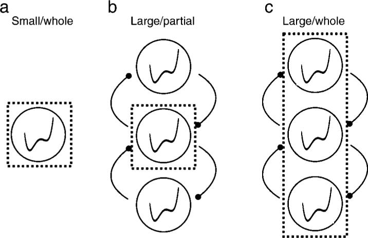
Illustration of the three models corresponding to the three experimental conditions (SW, LP, and LW). A single local rivalry indicates the binocular rivalry of the two small-sized rival stimuli (a) whereas three local rivalries with the interaction term comprise the binocular rivalry of the vertically elongated large rival stimuli (b and c). Dotted boxes indicate the hypothetical monitoring regions.
To create a network model of binocular rivalry from this energy model, the coupling term ηX(Ej, Ei) and the noise term ωni(t) are added as shown in Equation 2. As defined in Equation 3, X(Ej, Ei) governs the interaction between the perceptual states of the two local rivalries such that local rivalry i only interacts with the nearest other local rivalries j (NBi indicates the set of the nearest neighbors of the local rivalry i). Ki is the normalization factor, which corresponds to the number of neighboring local rivalries connected to the local rivalry i (but additional simulation without this normalization factor produced qualitatively similar results). [Ei] represents the perceptual state of the given local rivalry i, which is either +1 or −1. This ±1 value is used because the energy function has a local minimum at r ∼ ±1. Therefore, if the perceptual states of the two adjacent local rivalries are the same, this interaction does not influence Equation 2. The coupling strength of the network model is determined by η in Equation 2 and this η equals 0 for SW model (details about the model parameters and the simulation procedures are described in Appendix A).
The three (SW, LP, and LW) models were investigated by changing the key parameters of the simulation (gA, gB, and η). In Figure 4, line style (width and solid/dashed) indicates the dominance durations at a given contra-contrast gA whereas color indicates the coupling strength η as shown at the right of Figure 4c. First, gA and gB were varied among 0.1, 0.2, and 0.4 for the SW model. In the model, they correspond to the contrasts of the two rival stimuli. The mean dominance durations produced by the simulation of the single local rivalry were very similar to the experimental results (Figure 4a). This is consistent with the simulation of Moreno-Bote et al. (2007), confirming that the SW model produces dominance durations whose variation violates the contrast-invariant property of Levelt's 2nd proposition: increasing ipsi-contrast gB increases the mean dominance duration.
Figure 4.

Simulation results of dominance durations. Line style indicates the dominance durations at a given gA (thick line for gA = 0.1; dotted line for gA = 0.2; thin gray line for gA = 0.4) as a function of gB. The color of each line indicates the coupling strength from 0 to 0.25 by step size 0.05 as shown in the color bar at the right side of (c).
Now, the critical test of this simulation is to see whether the coupling strength η parameter inherent in the LP and LW models produces patterns of results mirroring those obtained from the experiments, especially the contrast-invariant property of Levelt's 2nd proposition. Figures 4b and 4c summarize the dominance durations of the LP and LW model, respectively. When η equals 0, the LP model's dominance durations are identical to the dominance durations of SW model, as they should be. Consistent with experimental results, dominance durations decrease with increasing gA at the same coupling strength η for all three models. In addition, as the coupling strength η increases, overall dominance durations decrease for LP and LW models compared to the SW model. Most importantly, with the properly selected coupling strength η, the mean dominance durations remain relatively unchanged at increasing ipsi-contrast gB and this pattern of result is particularly conspicuous for LW model. Thus, this simulated behavior of the LW model captures the contrast-invariant property of Levelt's 2nd proposition.
Discussion
The present study examined contrast-dependent dynamics of binocular rivalry for different sized rival targets. The most important empirical finding of the study showed that the contrast-invariant property of Levelt's 2nd proposition depends on the size of the rival stimuli, reconciling conflicting claims in the literature. In addition, a simple energy model with spatial coupling could reproduce the empirical findings of this study, suggesting that rivalry dynamics are the outcome of cooperative/competitive interactions among spatially distributed local zones of rivalries (Alais et al., 2006; Blake et al., 1992; Knapen et al., 2007; O'Shea et al., 1997; Wilson et al., 2001).
Why do large-sized rival stimuli produce the contrast-invariant property consistent with Levelt's 2nd proposition while small-sized rival stimuli violate this proposition? For purposes of answering this question, I will focus on the SW and LW conditions, for it is the results from those two conditions that highlight this seemingly contradictory behavior. One possible explanation for this size-dependent behavior emerges from consideration of two characteristics of binocular rivalry. First, we know that large-sized rival stimuli often produce mixed dominance states, whereas small-sized rival stimuli are less likely to produce mixed dominance. Mixed dominance states introduce the possibility of return transitions (RTs): state changes in which an exclusively dominant rival pattern temporarily enters a state of mixed dominance but then becomes exclusively dominant again. It stands to reason, then, that large rival targets are more likely to yield RTs than are small rival targets. Second, we know that the fraction of RTs systematically changes dependent on the contrast of rival stimuli (Brascamp et al., 2006). So it is reasonable to wonder whether the dependence of Levelt's 2nd proposition on size might be attributable to the differential incidence of RTs associated with SW and LW. The analyses in the following section evaluate this possibility.
Dynamics of return transitions
I analyzed the fraction of return transitions (FRTs: proportion of RTs out of all transitions) for the SW and LW conditions. To evaluate the dependence of RTs on contrast, I borrowed the concept of “departure” contrast as used by Brascamp et al. (2006): “departure” contrast refers to the contrast of the dominant pattern before an RT. I will refer to the contrast of the other stimulus, i.e., the one that did not achieve complete dominance following the mixed dominance state, as “companion contrast.” In Figure 5, the departure contrast is represented along the x-axis and companion contrast is represented by the color of three lines. Consistent with Brascamp et al. (2006), the FRTs increased with departure contrast and decreased with increasing companion contrast [three-way ANOVA with factor of two experimental conditions (SW and LW) × departure contrast × companion contrast showed significant effect of the departure contrast F(1,7) = 8.45, p < 0.5 and companion contrast F(1,7) = 14.86, p < 0.01]. This observation is most pronounced at the highest departure contrast and the lowest companion contrast. Importantly, the RTs occur in similar proportions for both SW and LW conditions [F(1,7) = 2.75, p = 0.14], suggesting that the incidence of RTs cannot explain the contrast-invariant property of Levelt's 2nd proposition. To provide converging evidence for this tentative conclusion, I performed additional analyses of the dynamics of RTs for these two conditions.
Figure 5.

FRTs (Fraction of Return Transitions) of the two experimental conditions (SW and LW). The x-axis represents the departure contrast and the three lines represent the companion contrast (red line for 1×; green line for 2×; blue line for 4×). Error bar equals ±SE.
To begin, I computed predominance for each of the contrast pairings in both tracking conditions (SW and LW); predominance is defined as the sum of all dominance durations associated with the ipsilateral stimulus divided by total duration of a tracking period. Those predominance values are shown in Figure 6, and here it can be seen that predominance of the ipsilateral stimulus increased with ipsilateral contrast for both conditions. This means, in other words, that predominance does not mirror the effect of ipsilateral contrast on average dominance durations (Figure 2), for those average durations increased only for the SW condition. Is it possible that RTs are responsible for this difference in behavior between predominance and average dominance durations?
Figure 6.

Predominance of the two experimental conditions (SW and LW). The x-axis represents the contrast of the ipsilateral stimulus and the three lines represent the contrast of the contralateral stimulus whose colors are the same as Figure 2. Error bar equals ±SE.
To answer this question, I compared the predominance and the average dominance durations for two categories of dominance states:
those associated with RTs, and
those associated with alternation transitions (ATs), i.e., episodes in which dominance switched from one stimulus to the other.
The first category, then, consists of dominance durations associated with episodes where a stimulus was dominant, it transitioned to the mixed state and it then transitioned back to dominance—the durations associated with that second, return state constitute RT durations. The second category, ATs, consists of dominance durations associated with episodes where one stimulus was dominant followed by dominance of the other stimulus (irrespective of whether a mixture occurred in between)—the durations associated with that second dominance state constitute AT durations. With these two categories of dominance durations established, I computed mean dominance duration and predominance for all contrast pairs for both of the tracking conditions. Those results are shown in Figure 7, with the dynamics of RTs shown by the dotted lines and the dynamics of ATs shown by the solid lines.
Figure 7.

Dynamics of ATs (alternation transitions) and RTs (return transitions) of the two experimental conditions (SW and LW). (a) and (b) show the predominance and (c) and (d) show the mean dominance durations. The solid lines present the measures obtained from ATs and the dotted lines represent the measures obtained from the RTs. The x-axis represents the contrast of the ipsilateral stimulus and the three lines represent the contrast of the contralateral stimulus whose colors are the same as Figure 2. Error bar equals ±SE.
Figures 7a and 7b show the dynamics associated with the predominance of the SW and LW conditions, respectively. Considering first the RTs (dotted lines), as ipsi-contrast level increased, the predominance associated with these RTs increased [with two-way ANOVA with factors of ipsi- and contra-contrasts, F(1,7) = 58.10, p < 0.001 for the SW condition; F(1,7) = 9.20, p < 0.05 for the LW condition]. This pattern of results is particularly conspicuous at low contra-contrast and high ipsi-contrast levels, accounting for much of the increased predominance shown in Figure 6. However, the mean dominance durations of ATs and RTs, shown in Figures 7c and 7d, change similarly as a function of ipsi-contrast level: when the ipsi-contrast level increases, the mean dominance durations associated with both the ATs and RTs increase for the SW condition but remain unchanged for the LW condition. An ANOVA with three factors (transition type, ipsi-contrast, and contra-contrast) shows no significant interactions between the transition type and ipsi-contrast [F(1,7) = 0.71, p = 0.43 for the SW condition; F(1,7) = 0.08, p < 0.5 for the LW condition]. Thus, the contrast-invariant property of Levelt's 2nd proposition observed with large rival stimuli is not accounted for by mean dominance durations associated with RTs.
Spatiotemporal dynamics during binocular rivalry
The empirical results in this paper confirm that rival stimulus size is an important factor determining rival dynamics (Figure 2). Moreover, the simulations in this paper demonstrate that network models of rivalry can reproduce these empirical results (Figure 4). Those models work because of coupling among neighboring zones of rivalry that entrain equivalent states within those zones: couplings embody the size-dependent behavior measured perceptually. The model I implemented, however, is undoubtedly oversimplified. For example, the sizes of the zones were arbitrary and were not scaled for retinal eccentricity, which they should be to conform with known properties of early visual mechanisms. A more refined version of this model needs to take into account other factors, as well. These include connection topology (e.g., longer connection for the collinear pattern; Wilson et al., 2001) and noise statistics (Lindner et al., 1998; Stollenwerk & Bode, 2003; Zhang et al., 1998).
Finally, a successful model must accommodate the influence of stimulus complexity on rivalry dynamics, including the dynamics specified by Levelt's 2nd proposition. Very little is known about these kinds of influences, although there is some hint in the literature that they matter. Specifically, Meng and Tong (2004) measured rivalry alternations using large dichoptic stimuli comprising pictures of a house and a face. They varied the contrast levels of these stimuli and found that increasing the ipsi-contrast increased mean dominance durations, a violation of the contrast-invariant part of Levelt's 2nd proposition. As shown in my experiments (Figure 2) and in the other studies listed in Table 1, however, large rival stimuli comprising simple figures do obey Levelt's 2nd proposition. It may be, then, that the sizes of the zones of rivalry forming a network and the strength of the coupling among those zones vary with stimulus complexity. This possibility is not far-fetched, based on the notion that rivalry transpires at multiple levels within the visual hierarchy (Blake & Logothetis, 2002; Freeman, 2005; Logothetis et al., 1996; Nguyen, Freeman, & Alais, 2003; van Boxtel, Alais, & van Ee, 2008).
Conclusion
The present paper shows that the contrast-invariant property of Levelt's 2nd proposition appears by increasing the size of stimuli. This result reconciles the conflicting claims of previous literature. The present empirical and modeling studies shed light on how to consider the dynamics of binocular rivalry.
Acknowledgments
I thank Randolph Blake for help in all phases of this project. I also thank Jan Brascamp, Moreno-Bote Ruben, and Sam Ling for helpful comments on the data analysis, simulation process, and manuscript preparation. This study was supported by NIH grants P30-EY008126, EY-13358, and EY-016752.
Appendix A
The overall simulation procedure and many details are similar to those of Moreno-Bote et al. (2007), and the units in the simulations are arbitrary. The energy model is defined by a double-well energy function shown in Equation 1 and its dynamics are governed by the differential shown in Equation 2 whose time constant τ = 10. According to Moreno-Bote et al. (2007), the noise term ni(t) in Equation 2 follows Ornstein–Uhlenbeck process whose amplitude was increased by ω = 5. In this equation, the time constant τs = 100, deviation term σ = 0.7, and ξi(t) represents a white noise randomly selected from a normal distribution. Euler's method was used for all numerical integration with time step δt equals 0.1 for 106 time unit, which means for 107 iterations. Matlab (Mathworks, MA) running in Machintosh G5 computer (Apple, CA) was used for the simulation.
Footnotes
Commercial relationships: none.
References
- Alais D, Lorenceau J, Arrighi R, Cass J. Contour interactions between pairs of Gabors engaged in binocular rivalry reveal a map of the association field. Vision Research. 2006;46:1473–1487. doi: 10.1016/j.visres.2005.09.029. [PubMed] [DOI] [PubMed] [Google Scholar]
- Blake R. Threshold conditions for binocular rivalry. Journal of Experimental Psychology: Human Perception and Performance. 1977;3:251–257. doi: 10.1037//0096-1523.3.2.251. [PubMed] [DOI] [PubMed] [Google Scholar]
- Blake R. A neural theory of binocular rivalry. Psychological Review. 1989;96:145–167. doi: 10.1037/0033-295x.96.1.145. [PubMed] [DOI] [PubMed] [Google Scholar]
- Blake R. A primer on binocular rivalry, including current controversies. Brain and Mind. 2001;2:5–38. [Google Scholar]
- Blake R, Logothetis NK. Visual competition. Nature Reviews, Neuroscience. 2002;3:13–21. doi: 10.1038/nrn701. [PubMed] [DOI] [PubMed] [Google Scholar]
- Blake R, O'Shea RP, Mueller TJ. Spatial zones of binocular rivalry in central and peripheral vision. Visual Neuroscience. 1992;8:469–478. doi: 10.1017/s0952523800004971. [PubMed] [DOI] [PubMed] [Google Scholar]
- Bossink CJ, Stalmeier PF, De Weert CM. A test of Levelt's second proposition for binocular rivalry. Vision Research. 1993;33:1413–1419. doi: 10.1016/0042-6989(93)90047-z. [PubMed] [DOI] [PubMed] [Google Scholar]
- Brainard DH. The Psychophysics Toolbox. Spatial Vision. 1997;10:433–436. [PubMed] [PubMed] [Google Scholar]
- Brascamp JW, van Ee R, Noest AJ, Jacobs RH, van den Berg AV. The time course of binocular rivalry reveals a fundamental role of noise. Journal of Vision. 2006;6(11):8, 1244–1256. doi: 10.1167/6.11.8. http://journalofvision.org/6/11/8/, doi:10.1167/6.11.8. [PubMed][Article] [DOI] [PubMed]
- Brascamp JW, van Ee R, Pestman WR, van den Berg AV. Distributions of alternation rates in various forms of bistable perception. Journal of Vision. 2005;5(4):1, 287–298. doi: 10.1167/5.4.1. http://journalofvision.org/5/4/1/, doi:10.1167/5.4.1. [PubMed][Article] [DOI] [PubMed]
- Fox R, Herrmann J. Stochastic properties of binocular rivalry alternations. Perception & Psychophysics. 1967;2:432–436. [Google Scholar]
- Fox R, Rasche F. Binocular rivalry and reciprocal inhibition. Perception & Psychophysics. 1969;5:215–217. [Google Scholar]
- Freeman AW. Multistage model for binocular rivalry. Journal of Neurophysiology. 2005;94:4412–4420. doi: 10.1152/jn.00557.2005. [PubMed][Article] [DOI] [PubMed] [Google Scholar]
- Hupé JM, Rubin N. The dynamics of bistable alternation in ambiguous motion displays: A fresh look at plaids. Vision Research. 2003;43:531–548. doi: 10.1016/s0042-6989(02)00593-x. [PubMed] [DOI] [PubMed] [Google Scholar]
- Kalarickal JK, Marshall JA. Neural model of temporal and stochastic properties of binocular rivalry. Neurocomputing. 2000;32–33:843–853. [Google Scholar]
- Kim YJ, Grabowecky M, Suzuki S. Stochastic resonance in binocular rivalry. Vision Research. 2006;46:392–406. doi: 10.1016/j.visres.2005.08.009. [PubMed] [DOI] [PubMed] [Google Scholar]
- Knapen T, van Ee R, Blake R. Stimulus motion propels traveling waves in binocular rivalry. PLoS ONE. 2007;2:e739. doi: 10.1371/journal.pone.0000739. [PubMed][Article] [DOI] [PMC free article] [PubMed] [Google Scholar]
- Laing CR, Chow CC. A spiking neuron model for binocular rivalry. Journal of Computational Neuroscience. 2002;12:39–53. doi: 10.1023/a:1014942129705. [PubMed] [DOI] [PubMed] [Google Scholar]
- Lehky SR. An astable multivibrator model of binocular rivalry. Perception. 1988;17:215–228. doi: 10.1068/p170215. [PubMed] [DOI] [PubMed] [Google Scholar]
- Lehky SR. Binocular rivalry is not chaotic. Proceedings of the Royal Society B: Biological Sciences. 1995;259:71–76. doi: 10.1098/rspb.1995.0011. [PubMed][Article] [DOI] [PubMed] [Google Scholar]
- Levelt W. Soesterberg. Institution for Perception RVO-TNO; The Netherlands: 1965. On binocular rivalry. [Google Scholar]
- Lindner JF, Chandramouli S, Bulsara AR, Löcher M, Ditto W. Noise enhanced propagation. Physical Review Letters. 1998;81:5048–5051. [Google Scholar]
- Logothetis NK, Leopold DA, Sheinberg DL. What is rivalling during binocular rivalry? Nature. 1996;380:621–624. doi: 10.1038/380621a0. [PubMed] [DOI] [PubMed] [Google Scholar]
- Meng M, Tong F. Can attention selectively bias bistable perception? Differences between binocular rivalry and ambiguous figures. Journal of Vision. 2004;4(7):2, 539–551. doi: 10.1167/4.7.2. http://journalofvision.org/4/7/2/, doi:10.1167/4.7.2. [PubMed][Article] [DOI] [PMC free article] [PubMed]
- Moreno-Bote R, Rinzel J, Rubin N. Noise-induced alternations in an attractor network model of perceptual bistability. Journal of Neurophysiology. 2007;98:1125–1139. doi: 10.1152/jn.00116.2007. [PubMed][Article] [DOI] [PMC free article] [PubMed] [Google Scholar]
- Mueller TJ, Blake R. A fresh look at the temporal dynamics of binocular rivalry. Biological Cybernetics. 1989;61:223–232. doi: 10.1007/BF00198769. [PubMed] [DOI] [PubMed] [Google Scholar]
- Nguyen VA, Freeman AW, Alais D. Increasing depth of binocular rivalry suppression along two visual pathways. Vision Research. 2003;43:2003–2008. doi: 10.1016/s0042-6989(03)00314-6. [PubMed] [DOI] [PubMed] [Google Scholar]
- O'Shea RP, Sim AJ, Govan DG. The effect of spatial frequency and field size on the spread of exclusive visibility in binocular rivalry. Vision Research. 1997;37:175–183. doi: 10.1016/s0042-6989(96)00113-7. [PubMed] [DOI] [PubMed] [Google Scholar]
- Pelli DG. The VideoToolbox software for visual psychophysics: Transforming numbers into movies. Spatial Vision. 1997;10:437–442. [PubMed] [PubMed] [Google Scholar]
- Stollenwerk L, Bode M. Lateral neural model of binocular rivalry. Neural Computation. 2003;15:2863–2882. doi: 10.1162/089976603322518777. [PubMed] [DOI] [PubMed] [Google Scholar]
- van Boxtel JJ, Alais D, van Ee R. Retinotopic and non-retinotopic stimulus encoding in binocular rivalry and the involvement of feedback. Journal of Vision. 2008;8(5):17, 1–10. doi: 10.1167/8.5.17. http://journalofvision.org/8/5/17/, doi:10.1167/8.5.17. [PubMed][Article] [DOI] [PubMed]
- Wilson HR. Computational evidence for a rivalry hierarchy in vision. Proceedings of the National Academy of Sciences of the United States of America. 2003;100:14499–14503. doi: 10.1073/pnas.2333622100. [PubMed][Article] [DOI] [PMC free article] [PubMed] [Google Scholar]
- Wilson HR, Blake R, Lee SH. Dynamics of travelling waves in visual perception. Nature. 2001;412:907–910. doi: 10.1038/35091066. [PubMed] [DOI] [PubMed] [Google Scholar]
- Zhang Y, Hu G, Gammaitoni L. Signal transmission in one-way coupled bistable systems: Noise effect. Physical Review E. 1998;58:2952–2956. [Google Scholar]