A Quantitative Explanation of Responses to Disparity-Defined Edges in Macaque V2

Abstract

Previous experiments have shown that V2 neurons respond to complex stimuli such as cyclopean edges (edges defined purely by binocular disparity), angles, and motion borders. It is currently unknown whether these responses are a simple consequence of converging inputs from a prior stage of processing (V1). Alternatively, they may identify edges in a way that is invariant across a range of visual cues defining the edge, in which case they could provide a neuronal substrate for scene segmentation. Here, we examine the ability of a simple feedforward model that combines two V1-like inputs to describe the responses of V2 neurons to cyclopean edges. A linear feedforward model was able to qualitatively reproduce the major patterns of response enhancement for cyclopean edges seen in V2. However, quantitative fitting revealed that this model usually predicts response suppression by some edge configurations and such suppression was rarely seen in the data. This problem was resolved by introducing a squaring nonlinearity at the output of the individual inputs prior to combination. The extended model produced extremely good fits to most of our data. We conclude that the responses of V2 neurons to complex stimuli such as cyclopean edges can be adequately explained by a simple convergence model and do not necessarily represent the development of sophisticated mechanisms that signal scene segmentation, although they probably constitute a step toward this goal.

INTRODUCTION

Recent evidence suggests that neurons in primate V2 have responses that are selective for discontinuities of various stimulus attributes in their receptive fields (RFs) such as angles (Haynes et al. 2004; Ito and Komatsu 2004), edges defined only by discontinuities in horizontal disparity (cyclopean edges) (Bredfeldt and Cumming 2006; von der Heydt et al. 2000; Zhou et al. 2000), and motion borders (Marcar et al. 2000). This response pattern is a marked departure from the properties of V1 cells, which respond primarily to variation in luminance and are generally spatially homogeneous for other stimulus properties such as orientation, disparity, and motion (Hubel and Wiesel 1962; Nienborg et al. 2004). The result is that single neurons in V2 are able to signal the presence of more complex features than single neurons in V1. These signals may ultimately be used for high-level perceptual tasks, such as figure–ground segregation (Qiu and von der Heydt 2005). It is even possible that the measured V2 responses could form the neural substrate for such subtle perceptual judgments, i.e., that V2 neurons respond to all edges that represent a perceived figure–ground boundary and only to such edges. In this case the response would be expected to be independent of how the boundary was defined (e.g., by disparity, luminance, and motion direction) and of the precise disparities (luminances, etc.) on either side of the edge. Such a response would have to draw on stimulus information from well outside the neuron's classical receptive field.

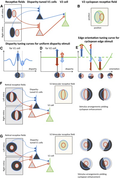
An alternative possibility is that the observed V2 responses compute a relatively simple function of the retinal stimulus within the receptive field. A purely feedforward mechanism as simple as combining the responses of several V1 neurons [similar to the way in which Hubel and Wiesel (1962) proposed that simple cells are constructed from the responses of LGN neurons] might suffice to explain observed neuronal responses in V2. Several groups have previously suggested that this type of model could potentially explain angle selectivity (Boynton and Hegde 2004; Ito and Komatsu 2004) and selectivity for complex spatial stimuli (Hegde and Van Essen 2000). However, to date there has been no quantitative analysis of how well these simple models account for the neuronal data and it is therefore not yet clear that such simple explanations of responses to complex stimuli are adequate. Here we perform such a quantitative evaluation of our recent data demonstrating responses of V2 neurons to edges defined only by disparity (Bredfeldt and Cumming 2006). These data are rich enough (a total of 62 edge conditions were measured for each cell) to provide an adequate test for simple feedforward models. We described broadly three types of responses (very similar to those originally described by von der Heydt et al. 2000), each of which could be explained qualitatively by supposing that they result simply from combining the responses of two disparity-selective V1 neurons that have different preferred disparities. First, some neurons respond to a disparity-defined edge at one orientation, but do not respond to the same edge when the disparities are swapped (responses to only one disparity sign). This pattern can be produced by combining the output of two V1 neurons with receptive fields that are slightly displaced (Fig. 1, A–E). Second, many neurons respond to both signs of a particular orientation of the cyclopean edge. This pattern can be produced by combining the output of two V1 neurons of different sizes, as illustrated in Fig. 1F. Finally, a substantial proportion of neurons respond to all edge orientations more strongly that to either disparity alone. These might be explained with a concentric arrangement of receptive fields, like that shown in Fig. 1G.

FIG. 1.

Diagram of the model. Two disparity-selective V1 cells (red and blue triangles) with different disparity tuning, position, and size converge on a single V2 cell (green triangle). The retinal receptive fields of each V1 cell are shown on the retinas (A), colored-coded red and blue according to the V1 cell they project to. The receptive fields are at different locations on the retina, but have the same position offset between left and right eyes. The red and blue cells’ inputs to the V2 cell differ in sign. B: the receptive field of the V2 cell in cyclopean visual space. The region shaded green shows visual directions where the cell is sensitive to stimuli. The blue and red subregions show the cyclopean receptive fields of the component V1 cells. C: the disparity tuning curve for the blue V1 cell, in response to stimuli with uniform disparity. Two example stimuli are shown along the horizontal axis; we use dark and light gray to represent the preferred and null different disparities of this V1 cell. The cyclopean position of the blue receptive field is superimposed. The disparity tuning curve for the red V1 cell would be the same, but upside-down. Thus the dark-shaded disparity is the null disparity of the red V1 cell, whereas the light-shaded disparity is its preferred disparity. D: the disparity tuning curve that would be obtained from the green V2 cell. The response is constant, i.e., the V2 cell shows no tuning to uniform disparity stimuli. This is because the inputs from the two V1 subunits are always equal and opposite, as indicated by the red and blue arrows in D (in this simplified linear model, each model V1 cell is imagined to be capable of providing both positive and negative output; a more physiologically realistic model would achieve the same result using a push–pull pair of cells). For the dark-shaded disparity, the blue cell provides strong positive input but the red cell provides equally strong negative input, relative to the response to uncorrelated stimuli. For the light-shaded disparity, the blue cell provides weak negative input, whereas the red cell provides weak positive input. The net result is the same. E: the response of the V2 cell to cyclopean edge stimuli, made up of the light- and dark-shaded disparities selected in C but with different edge orientations. Four example stimuli are shown along the horizontal axis, with the cyclopean receptive fields of the V1 subunits superimposed. The first stimulus has a vertical edge and both V1 subunits are completely covered by their preferred disparities. The V2 response is therefore the sum of 2 positive V1 responses, showing cyclopean enhancement above the response to uniform disparities. With a horizontal edge, each subunit is covered half by its preferred disparity and half by its null disparity (thus the half-arrows in E). The increase in response driven by the preferred disparity is cancelled out by the decrease driven by the null disparity, so the total response of each subunit is the same as that for uniform stimuli. The V2 cell therefore shows no cyclopean enhancement above or below the response to uniform disparities. When the edge is vertical but the disparities are on the other side, each V1 subunit is covered by its null disparity, so the response is minimized. Thus this organization produces enhanced cyclopean response for only one edge sign. F: diagram illustrating an organization that can produce enhanced responses for 2 different edge signs. In the configuration shown, the central red subfield is covered with its preferred disparity, whereas the blue subfield is covered by a mixture of both disparities. The summed response is greater than that to a uniform disparity. If the disparities are swapped and the edge is moved to the other side of the central subfield, the same enhancement results. G: concentric subunits lead to cyclopean edge responses for all orientations so long as the central subfield is just covered by its preferred disparity.

Each of these qualitative explanations invokes only two V1-like subunits, which differ in their response to the two disparities defining the edge. Note that these schemes describing the arrangement of the input subunits provide only an explanation of how certain orientations and signs of cyclopean edges can produce a stronger response than either disparity alone. It may be that other aspects of the response are not compatible with such simple schemes. Only quantitative modeling of the whole response can determine whether the simple schemes are adequate. Indeed we will show that in most cases the simplest form of this model is not compatible with the observed responses, but a minor modification produces a very good description. We conclude that a simple feedforward model can explain the pattern of cyclopean edge responses in V2. We suggest that other tuning characteristics (i.e., tuning for motion borders and angle stimuli) might be similarly explained by assigning different motion and orientation selectivity to the subunits.

METHODS

Data collection

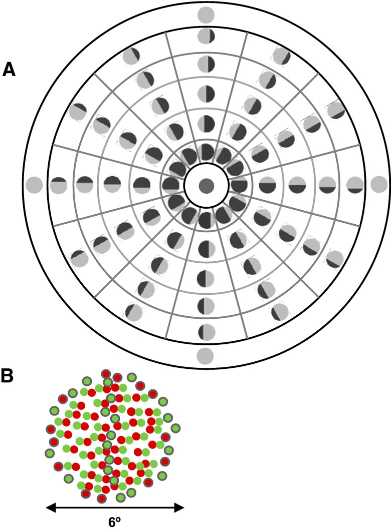
The data collection is described in detail by Bredfeldt and Cumming (2006). In brief, extracellular recordings of single units from V2 of awake macaques were made while stereograms were presented via a haploscope. The location of the RF center was initially determined with interactively positioned bars and luminance gratings and then quantitatively mapped by presenting thin strips of luminance gratings at different locations (Read and Cumming 2003). Random-dot stereograms 5° in diameter (larger than all the RF diameters) were then centered on this location. The stereograms were divided into two halves by a single edge and defined only by a difference in horizontal disparity between the two sides of the stereogram. Binocularly, the stimulus appears as two half-discs, floating at different depths. The disparity-defined edge was presented at six orientations (separated by 30°), and at five locations (separated by 0.55°) for each orientation. Figure 2A shows the stimuli used in the experiment. Light gray and dark gray are used to represent the two component disparities that make up the edge. Swapping the two disparities across the edge is defined to be changing the “sign” of the disparity edge. The stimuli are arranged on the polar axes used to present results both here and in a previous study (Bredfeldt and Cumming 2006). The axes are divided radially into segments and concentrically into rings. The center of the plot and the outermost ring represent control stimuli with uniform disparity. Stimuli drawn in the same ring have edges at the same distance from the center of the receptive field. Stimuli within a given radial segment have the same edge orientation, e.g., vertical or horizontal. Stimuli 180° apart, i.e., in opposite segments but at the same radial distance from the center, have edges with the same orientation but with opposite disparity signs and with locations on opposite side of the center. Note that the same set of cyclopean edge orientations were used in all cells, regardless of the preferred orientation for luminance-defined contours.

FIG. 2.

Stimulus used to record responses to cyclopean edges. A: polar axes used throughout this study and its predecessor (Bredfeldt and Cumming 2006) to represent edge orientation and position. The icon in each segment shows the corresponding stimulus. B: example of a random-dot stimulus containing a cyclopean edge. Red and green dots represent the inputs to the right and left eyes, respectively. Note that in the left half of the stimulus, green dots are shifted to the left of the red dots, whereas in the right half of the stimulus green dots are shifted to the right half of the stimulus. This creates a disparity-defined vertical edge. Gaps in the stimulus (caused by application of disparity to the dots) were filled with uncorrelated dots, shown here with black outlines. Note that green and red dots are shown here for illustrative purposes. In the actual experiment, all dots were black or white.

All neurons that showed significantly stronger responses to disparity-defined edges than to uniform disparity fields (for details, see Bredfeldt and Cumming 2006) and whose responses passed a one-way ANOVA (P < 0.05) for the effect of cyclopean edge configuration were entered into the current study. The choice of the two disparity values was not based on the responses to disparity in a uniform random-dot stereogram (RDS) (many neurons showed no disparity selectivity under these circumstances). We relied on an initial exploration of different disparity-defined edges by hand to identify a combination that produced audible activation.

Model details

The model consists of two subunits with different positions, sizes, and disparity responses, which converge on a single V2 cell. In reality it is likely that more than two subunits converge on a single V2 cell. However, since our stimuli contained only two disparities, a model with two subunits should be sufficient to describe differential responses to the two disparities, whereas adding more subunits would risk overfitting. The model subunits behave like the binocular energy model, which provides a good account of the properties of binocular neurons in striate cortex. For the purposes of this study, the binocular energy model has an important property: the response to an RDS containing two disparities is simply the mean of the responses to each disparity alone, weighted by the fraction of the RF covered by each disparity. Thus it is not necessary to implement a full binocular energy model: we need to know only the response of each subunit to each disparity (S1_d1, S1_d2, S2_d1, S2_d2) and the shape of each subunit RF. The response of subunit 1 to the cyclopean edge stimulus is then given by

(1)

where S1_d1 and S1_d2 are the responses to the two disparities and A_S1 is the proportion of the receptive field covered by disparity 1. For simplicity, the model ignores the fact that, for some orientations, the stimulus may contain a small uncorrelated region (see following text); thus the proportion of the receptive field covered by disparity 2 is (1 − A_S1). Figure 3 shows a schematic of the model with all spatial parameters indicated. A_S1 is calculated by integrating the volume of the two-dimensional Gaussian S1 over the region covered by disparity 1. The outer limits of the integration were determined by the size of the stimulus previously used in our physiological experiments. The final response of the model is the difference of the responses of the two subunits passed through an output nonlinearity, half-wave rectification followed by an exponent

(2)

FIG. 3.

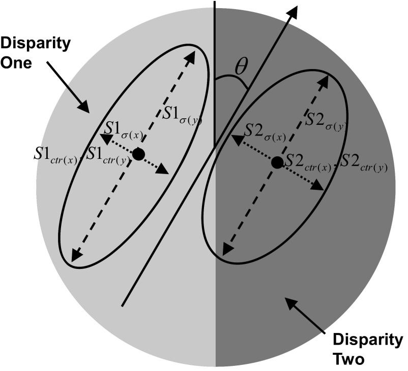
Pictorial representation of the spatial parameters used in the model: θ, orientation of subunits; S1_σ(x), SD x, subunit 1; S1_σ(y), SD y, subunit 1; S2_σ(x), SD x, subunit 2; S2_σ(y), SD y, subunit 2; S1_ctr(x), Location x, subunit 1; S1_ctr(y), Location y, subunit 1; S2_ctr(x), Location x, subunit 2; S2_ctr(y), Location y, subunit 2.

Since the two subunits are combined linearly, the choice of a minus sign in the middle of Eq. 2, as opposed to a plus sign, is immaterial. We refer to Eq. 2 as the Linear Summation (LS) model. Equation 2 can be rearranged and simplified as follows

(3)

The terms (S1_d1 − S1_d2), (S2_d1 − S2_d2), and (S1_d2 + S2_d2) are constants and so each represents only one free parameter in the fit. Thus the LS model contains a total of 13 parameters, used to describe 62 data points. These are (Fig. 3):

• Positions of subregions 1 and 2: S1_ctr(x), S1_ctr(y), S2_ctr(x), S2_ctr(y)

• Extents of subregions 1 and 2: S1_σ(x), S1_σ(y), S2_σ(x), S2_σ(y)

• Orientation of both subregions: θ

• Difference in responses of subregion 1 to the two disparities: (S1_d1 − S1_d2)

• Difference in responses of subregion 2 to the two disparities: (S2_d1 − S2_d2)

• Difference in responses of the two subregions to disparity 2: (S1_d2 − S2_d2)

• Output exponent: n

In the results, we explore an extension to this model that adds one parameter, but allows us to explore the effect of output nonlinearities on the subunits.

Stimulus details

We evaluated the model's response to cyclopean edge stimuli in which the edge was presented at the same range of orientations and positions used to collect the physiological data. The stimulus is a circular dynamic RDS 6° in diameter, where the central 5° contains two contiguous regions defined by different disparities. The border between the surfaces forms an edge in depth. Figure 2B illustrates a cyclopean edge stimulus with a vertical cyclopean edge in the center of the stimulus. Red and green dots represent the views of the right and left eyes, respectively; in the actual experiment all dots were black and white. The stimulus background, which consists of uncorrelated dots, hides the edges of the cyclopean edge stimulus to prevent monocular cues to orientation and edge location.

To create the vertical edge shown in Fig. 2B, the green dots have been shifted to the right on the right side of the edge and to the left on the left side of the edge. As a result, there is a gap in this area with no green dots, thus providing a cue to the location and orientation of the edge. To prevent such cues, the gap created by the horizontal shift is filled with uncorrelated green dots (uncorrelated dots are outlined in gray for clarity). This ensures that the dot density is uniform in both eyes’ views, regardless of disparity. Nonetheless, it is possible that a response to the lack of binocular correlation could cause a cell to appear orientation selective (since the size and position of the uncorrelated region change with orientation). However, we were careful to exclude this possibility when determining that a neuron shows a response that is specific for the disparity-defined edge. Consequently, we did not include the small effect produced by the uncorrelated dots in our modeling. (If responses to uncorrelated dots are included in the model, it introduces an extra parameter and one that can be exploited in an unrealistic way, with very large responses for both subunits, to fit certain response patterns.)

Quantitative modeling

We fit the model described earlier to the responses of 60 V2 neurons that showed significant responses to cyclopean edges. We imposed several constraints to ensure that fitted values would be physiologically plausible and computationally tractable. In particular, we set both lower and upper boundaries on the SDs of the individual subunit receptive fields. The lower boundary (0.275°) was determined by the measured edge position spacing, whereas the upper boundary (2.5°) was determined by the stimulus size (larger SDs would not produce an appreciable difference in the fitted values). In addition, the center of each subunit was required to lie inside the area covered by the stimulus. In a few instances, the model exploited extremely implausible output nonlinearities. To prevent this, the output exponent (n in Eqs. 2 and 3) was not allowed to exceed a value of 40.

Finally, because the variance in neuronal spike counts increases in proportion to the mean count, we fit the square root of the model's equations to the square root of the firing rate, thus eliminating dependence of the variance on the count (Prince et al. 2002). All fits were optimized using a least-squares fitting procedure in Matlab 7.0.4.

Evaluating model fit

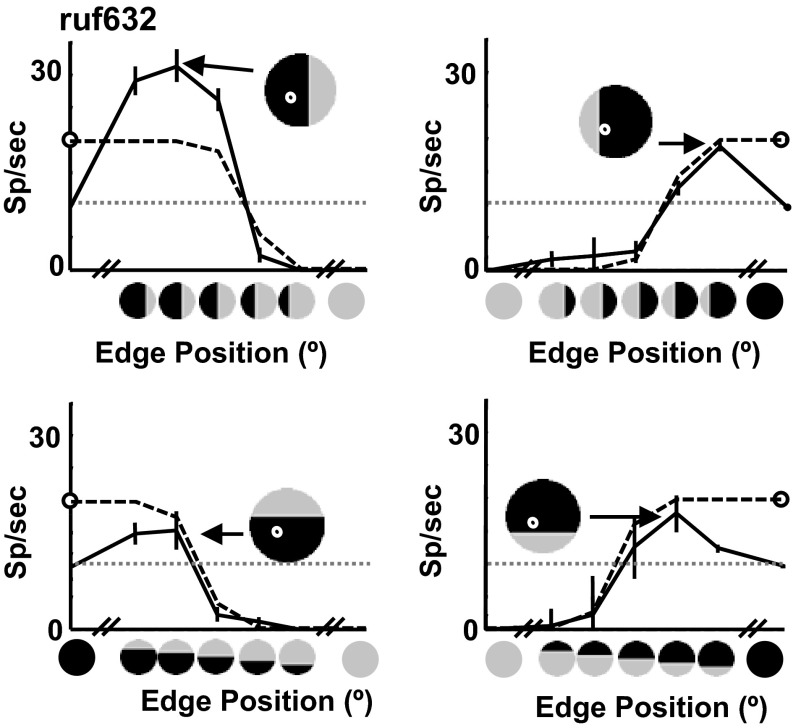
To quantify how well the model fit the V2 data, we measured the proportion of variance between mean responses (signal variance) that was explained by the fit. However, in many cases this simple metric could be misleading. In cases where much of the signal variance is explained by differences in the response to the two uniform disparities, even a single V1-like subunit can successfully explain a large proportion of the variance without explaining any of the response enhancement for cyclopean edges. Figure 4 provides an example of this phenomenon. Although the data show a clear cyclopean edge enhancement for both signs of a vertical edge and a horizontal edge, the cyclopean edge enhancement is small relative to the difference between the uniform disparity responses for all but one of the edge orientations/signs. Consequently, much of the variance is explained by a single subfield model that overestimates the response to one of the two uniform disparities (dashed line in Fig. 4; dotted line indicates the mean of the response, or the straight-line fit that would account for exactly zero of the signal variance). The single-subunit fit shown here explained 87% of the signal variance for the data shown in Fig. 4. Nonetheless, this single-subfield model fails to capture the cyclopean enhancement. Thus to understand how well a two-subfield model is able to explain the response to disparity-defined edges, we must first isolate that part of the response produced by the edges, not by their constituent disparities alone.

FIG. 4.

Example of a response in which most of the variance can be accounted for by a single subunit model. Solid lines indicate the observed responses; dashed lines indicate the fitted single subunit model. Dotted line represents the mean of the responses shown here. Stimulus inset shows the best- fitting receptive field for the single-subunit model. The model overestimates the response to one of the uniform disparities (marked with open symbol), which allows it to fit several points that show moderate cyclopean enhancement, as well as the points that fall between the 2 uniform disparity responses. For the data shown here, the single-subunit model can account for 87% of the signal variance, even though it does not capture the features of the response that demonstrate cyclopean edge enhancement.

To do this, we first fit both a single-subunit model and the two-subunit model to the raw data set. We then subtract the single-subfield model fit from both the data and the two-subfield model fit to obtain the portion of the response that cannot be explained by the single-subfield model. We refer to these differences as the cyclopean responses of the neuron (R_C) and the model fit (F_C) and compare their variance. In cases like that illustrated in Fig. 5 (bottom row), much of the response variance can be explained by a single subfield (no response lies far outside the range covered by the two uniform disparities). In such cases the magnitude of the cyclopean response, although significant, is not very much greater than the magnitude of the sampling noise. Consequently, even a perfect model would not be expected to explain 100% of the variance in R_C. Therefore we use the measured variability in data to estimate what fraction of the variance in R_C we can expect to explain.

FIG. 5.

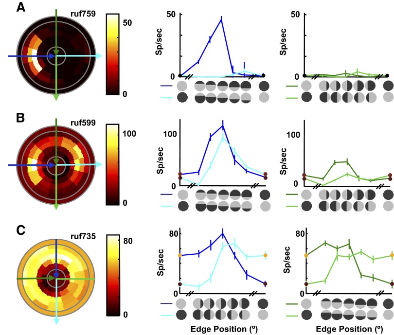
Examples of cyclopean edge responses previously recorded in V2 (Bredfeldt and Cumming 2006). For each example, responses to all edge configurations are shown in the pseudocolor plot on the left. As shown in Fig. 2A, the angular position of a patch (relative to the horizontal) represents stimulus orientation, whereas radial distance from the center represents edge position. The central disc and the outermost ring (delineated by solid gray lines) represent the response to control stimuli with uniform disparity. These conditions can be viewed as edge locations that lie outside the stimulus, as reflected by their radial location. The mapping between radial location and edge position can be more clearly seen in the cross sections shown to the right of the pseudocolor plot, which correspond to the blue and green arrows overlaid on the pseudocolor plot. The direction of each arrow indicates left-to-right on the cross-section graph. The cross section indicated in blue (middle column) shows responses at the preferred orientation, with the disparity sign that produced the strongest response represented in dark blue. The rightmost column (cross section representing the green arrows on the pseudocolor plot) shows responses to orientations orthogonal to the preferred. The stimulus icons along the x-axes indicate the edge orientation and position for each point in the plot. The 2 uniform horizontal disparities used to define the edge, d1 and d2, are shown as the extrema of the position tuning curve, and the symbol color matches the color for these data in the pseudocolor plot. A: orientation and sign tuned cyclopean edge response. B: neuron that responds to both signs of a preferred orientation edge. C: example that responds to all orientations of a cyclopean edge.

For each experimental condition, we calculate the variance associated with that mean and use the mean of these variances across all conditions to estimate the variance attributable to sampling noise, σ_err². The variance that we would expect a perfect model to explain is then var (R_C) − (N − n_p) × σ_err², where N is the number of stimulus conditions (62) and n_p is the number of parameters in the model (Haefner and Cumming, unpublished). When examining the cyclopean response after subtracting the best-fitting single-subunit model, n_p is the difference in the number of parameters between the one-subunit (8 parameters) and two-subunit models (13 parameters for the LS model).

RESULTS

This study assesses the ability of a simple feedforward model, combining two V1-like subunits, to capture the major characteristics of cyclopean edge tuning in macaque V2. We have previously described the responses of macaque V2 cells to cyclopean edges with a range of orientations and edge positions (Bredfeldt and Cumming 2006). Briefly, many V2 cells respond selectively to cyclopean edges, giving larger responses for the edge than they do for the component disparities that are used to create the edge. The examples in Fig. 5 capture the variation we found in response patterns. (Note that all examples shown herein are neurons different from those shown in Bredfeldt and Cumming 2006.) The pseudocolor plots (left columns) represent responses to all orientations and positions. As shown in Fig. 2A, the angular position of a patch represents edge orientation, whereas radial distance from the center represents edge position (with the middle of the five concentric rings representing an edge in the center of the stimulus). The central disc and the outermost ring represent the responses to the component disparities (control stimuli with uniform disparity). These can be viewed as conditions in which the edge location lies outside the stimulus, reflected by their radial location (see also cross sections in the rightmost columns of Fig. 5).

For each example (and for the examples throughout) the orientation that produced the maximum response is marked with blue arrows, whereas the orientation orthogonal to the preferred orientation is marked with green arrows (darker colors represent the sign of the edge that produced the larger response). The response at these orientations is replotted in the line plots in the two rightmost columns. This view makes it easier to see how cyclopean enhancement and suppression vary as a function of edge position, with the two disparity signs superimposed on the same line plots. The response is frequently tuned for edge orientation (Fig. 5A), although in general the tuning is weaker than that found in V1 for luminance-defined edges. We frequently observed responses to both signs of a disparity-defined edge, although the maximum response for each disparity sign usually occurred at different edge locations (Fig. 5B). However, a substantial proportion of cells showed very little orientation selectivity (Fig. 5C), despite showing stronger responses to disparity-defined edges than to either disparity.

Our model consists of two subunits that are combined at the level of V2 cells, followed by half-wave rectification and a variable output nonlinearity (a free parameter, n, in Eqs. 2 and 3). Figure 3 illustrates the model and lists the spatial parameters. Each subunit behaves like a binocular energy-model cell with a two-dimensional Gaussian receptive field envelope. The subunits differ in size, location, and in their responses to the two disparities contained in the stimulus, but are constrained to have the same orientation. The model would respond maximally if each subfield was stimulated solely by its preferred component disparity. Because the subunits generally overlap, this stimulus often could not be realized.

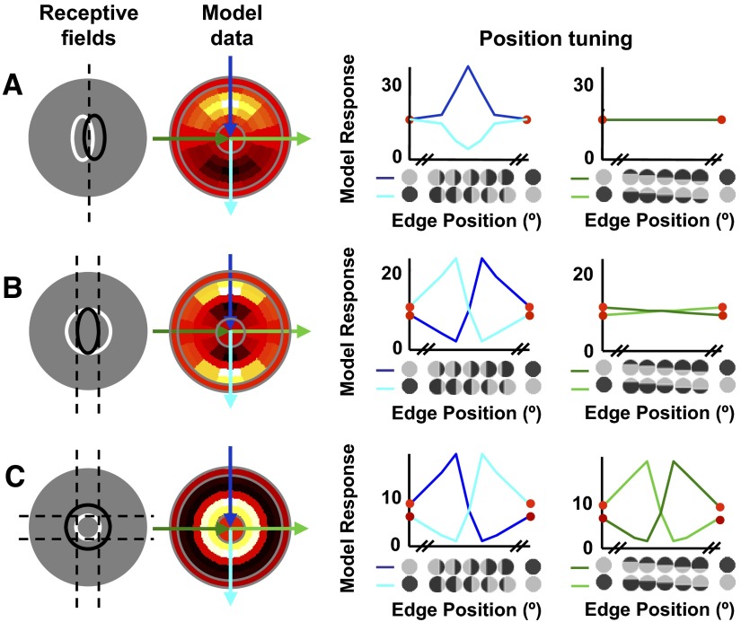
Figure 6 illustrates the model's output for three different spatial configurations that produce response patterns qualitatively similar to the example responses in Fig. 5. The leftmost column shows the arrangements of the two subunits (white and black lines, drawn at 1SD). The gray background represents the relative size and location of the stimulus.

FIG. 6.

Adjusting the size, shape, and locations of the subunits produces different patterns of cyclopean edge responses. Column 1: representation of the size and location of the subunits of the linear model, drawn at 1SD. Columns 2–4: example model responses, using the same plot conventions as in Fig. 3. A: elongating both subunits and organizing them in parallel produces a cyclopean peak for the preferred sign and suppression for the opposite sign of an edge in the same location. B and C: when one subunit surrounds the other, responses are produced for both signs of the edge. In B, one elongated and one circular subunit produce responses that are orientation tuned for both signs of the edge, provided the edge is appropriately positioned. When the central subunit is entirely covered by its preferred disparity, but the surrounding subunit still has a substantial fraction covered by its preferred disparity, enhancement (relative to uniform disparity) results (as in Fig. 1B). In C, a center–surround configuration produces both cyclopean responses at all edge orientations. In both B and C, the model shows cyclopean suppression as well as enhancement for all orientations that respond to the edge.

Figure 6A illustrates the case in which two elongated subunits are offset horizontally. This model cell is maximally stimulated by a vertical edge located between the two subunits (indicated by the dashed line). The line plot in the third column shows what happens as the vertical edge is swept across the model cell. When the edge is located at the far left of the stimulus, both subunits are stimulated with S1's preferred disparity and the model output is the linear combination of each subunit's response to that disparity. As the edge moves across the receptive field in the preferred direction, S2 begins to be stimulated with its own preferred disparity, leading to response enhancement. When the edge reaches the middle of the stimulus, both S1 and S2 are predominantly stimulated with their preferred disparities and the response enhancement reaches its peak. As the edge continues advancing, S1 becomes predominantly stimulated by its nonpreferred disparity and its response declines, leading to a decline in total model output. Swapping the disparities across the edge has a complementary effect: in this configuration, no edge location can stimulate both subunits with their preferred disparities. Rather, the central location predominantly stimulates both subunits with their nonpreferred disparity, causing response suppression that is maximal for a centrally located edge.

The second response pattern—that of orientation-tuned edge responses for both signs of a cyclopean edge—can be achieved by rearranging the model's subunits, as shown in Fig. 6B. In this case, a vertical edge to one side of the stimulus center (dashed lines) produces response enhancement, whereas the same edge reflected across the center of the stimulus produces strong response suppression. Swapping the disparities across the edge produces the same pattern of results, in complementary edge positions. Note that this model cell would produce a much stronger response for a cyclopean bar stimulus, which would stimulate both flanks of the larger subunit with its preferred disparity. Finally, the bottom row illustrates a center–surround subunit configuration, which produces cyclopean enhancement at all orientations and edge signs, similar to that seen in Fig. 5C.

Thus a simple linear combination of two V1-like subunits can qualitatively explain many aspects of the responses seen in V2 neurons to disparity-defined edges. However, one property of all three configurations in Fig. 6 does not match the responses of most neurons in the data set. For every configuration that produces an enhanced response, reversing the disparity sign produces substantial suppression (response rate lower than that of either disparity alone). The reason for this pattern is simple: net enhancement occurs when both subfields are stimulated predominantly with their preferred disparity. Swapping the disparities then means that both subunits are predominantly stimulated by the nonpreferred disparity. Although the output nonlinearity reduces the magnitude of the suppression (relative to response enhancement), it was still much stronger than was seen in real neurons. In real neurons, this cyclopean suppression was uncommon and, when it did occur, it tended to be considerably weaker than response enhancement for the preferred edge stimulus.

Quantitative modeling

As a result of this feature, the linear summation model did not account very well for the observed responses in many cases. In the few cases where the LS model did provide a good quantitative account (Fig. 7 illustrates three examples), this was usually because the neuronal responses showed weak cyclopean suppression at the predicted location and the asymmetry between the strength of enhancement and suppression could be captured by the effect of the expansive output nonlinearity (Fig. 7, A and C). The maximum fitted exponent for the LS model was 33.3, allowing the model to fit a substantial difference in the magnitude of cyclopean enhancement and suppression, although the median value was 2.5 (similar to previously described estimates of the output nonlinearity of cortical neurons; Anzai et al. 1999). In a number of additional cases, such as the example in Fig. 7B, the extremely low response to at least one of the component disparities allowed the predicted suppression in the model to be rectified; as a result, the model was able to fit large response peaks without large errors where suppression was not evident.

FIG. 7.

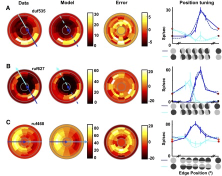
Example of 3 responses that are well fit by the linear model. Plotting conventions for the pseudocolor plots in columns 1–3 are the same as those used in Fig. 3. Third column shows the difference between the data and the model fit. Solid and dashed lines in the fourth column represent the position tuning of the preferred orientation edge for the data and model respectively. A: cell that is orientation and sign selective. This cell has a small amount of cyclopean suppression as shown by responses below the response to the less optimal control stimulus. B: responses to both edge signs, but at different locations. Note the response to one of the disparities is close to zero. Consequently, any suppression beneath this response predicted by the model is hidden by the rectification. C: response that shows orientation-selective enhancement for one edge sign and suppression for the opposite sign. Proportion of cyclopean variance explained that: 0.43, 0.31, and 0.49, respectively.

For each example, the complete data set is shown as a two-dimensional image map in the far left column of Fig. 7, whereas the best-fitting model response is shown in the second column. The third column displays the error between the data and the model response. Comparing the image maps for the data and the best-fitting model response for the examples in Fig. 7 reveals that the model was able to accurately capture the preferred orientation and sign and the preferred edge position. The edge location plot in the rightmost column of Fig. 7C shows the individual data points for the most responsive orientations (data: solid lines; model: dashed lines; opposite signs shown with dark and light blue).

We fit the model to the cyclopean edge responses of 60 macaque V2 cells, taken from the study of Bredfeldt and Cumming (2006). To quantitatively determine how well the model fit the data, we first factored out the amount of variance that could be accounted for by a single-subfield model, leaving the variance that can be attributed to the cyclopean signal (see methods for details). We then determined how much of the cyclopean signal variance could be explained by the two-subfield model. The model accounts, respectively, for 43, 31, and 49% of the cyclopean signal variance in the example cell data sets in Fig. 7 (86, 85, and 74% of the total signal variance).

For the majority of cells, the LS model explained substantially less of the cyclopean signal variance than in these examples. The examples in Fig. 8 show the limitation of using a simple output nonlinearity to minimize the suppression in the model's output: although it can reduce the magnitude of the expected suppression, it cannot predict a complete lack of suppression at that location. In Fig. 8A, the data show strong responses to both signs of an optimally oriented edge, but the peak responses both occur for edges in the center of the stimulus. Because the LS model must produce suppression for one sign of the edge at a given position, the model cannot fit this response and produces no significant cyclopean enhancement. Overall, for this cell the best-fitting two-subunit linear model was able to explain roughly 5% of the cyclopean response variance.

FIG. 8.

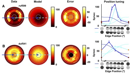
Example of 2 responses that are not well fit by the LS model. Figure conventions same as those used in Fig. 7. A: this response shows cyclopean edge enhancement for both edge signs for horizontal edges in the middle of the stimulus. Uniform disparity responses are elevated and there is little to no suppression. The model cannot show cyclopean enhancement for both signs of a cyclopean edge in the same edge positions. B: this example shows response enhancement to opposite edge signs in different locations, but shows no evidence of response suppression. The model fails to fit the data because it cannot fit both edge signs without showing complementary suppression, which is not seen in the data. As a result, the model predicts almost no cyclopean enhancement and explains almost none of the cyclopean variance (<0.05 in both cases).

Figure 8B provides an example of a nonorientation specific cell that is also poorly fit by the LS model. For this example cell, the maximum response occurs at different edge locations. However, at locations where one disparity sign produces enhancement, the opposite disparity sign still produces a response that is larger than the response to one of the uniform disparities, and thus cannot fit the linear summation of two energy models followed by an output exponent, which would predict suppression at this location.

A simple modification to the LS model

A relatively simple modification to the model allows it to reconcile the observed magnitudes of enhancement and suppression much more successfully. We simply propose that the output of each subunit is passed through an expansive nonlinearity (half-squaring) before the subunits are combined. Although we did not find it necessary to vary the value of this exponent, introducing this nonlinearity did introduce one extra free parameter to the model. In the LS model, any baseline activity in the subunits is equivalent to a single baseline term [(S1_d2 − S2_d2) in Eq. 3]. Once we introduce the squaring of subunit responses this is no longer true and S1_d2 and S2_d2 become independent parameters, introducing one more parameter to the fits

(4)

Since the combination of the subunits here is nonlinear (much like the way simple cell responses are summed in the energy model), we refer to this as the Nonlinear Summation (NS) model. Figure 9 shows that this model provides a much better account of the examples shown in Fig. 8 for the LS model. In particular, the NS model does not require that suppression occurs for edge signs opposite to those that produce response enhancement.

FIG. 9.

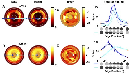
Fit of the nonlinear summation (NS) model for the 2 example cells shown in Fig. 8. Figure conventions are the same as those used in Fig. 7. The model is able to capture the peak for both signs of both example cells, without introducing complementary suppression that is not seen in the data. Proportion of cyclopean variance explained: 0.76 and 0.83, respectively.

Population analysis

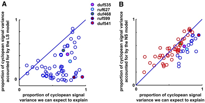
Figure 10 compares the success of the LS model and the NS model in describing the responses of 60 V2 neurons. Solid-colored points indicate example cells shown in Figs. 7–9. We use cyclopean signal variance to measure the quality of the fit rather than total signal variance; this allows us to estimate how much the two-subunit model improved the fit relative to a single-subunit model. However, for many cells the cyclopean signal variance was small relative to the total signal variance due to large differences in the responses to the two component disparities. For such cells, the magnitude of the cyclopean signal may not be much greater than the noise; thus for each model we compare the fraction of variance in the cyclopean response explained, against the fraction of variance we expect to explain with a perfect model (limited by noise; see methods). Points along the unity line indicate that the model was able to explain as much of the cyclopean signal variance as we would expect given the level of noise in the data.

FIG. 10.

Population results, for linear summation (LS) model (A) and NS model (B). Filled points indicate example cells (see legend). See methods for how we calculate cyclopean signal variance and the proportion of variance we can expect to explain. Neurons for which cyclopean enhancement was large relative to variability lie to the right in each plot. In B, red data points indicate individual cells in which a χ² test revealed no significant deviation from the NS model.

The LS model did a poor job of describing the data and most data points lay well beneath the identity line (Fig. 10A). In 40/60 cases, the fit was able to explain <25% of the cyclopean signal variance. For the 20 cells in which the fit was able to explain >25% of the cyclopean signal variance, 12 had responses near zero to at least one component disparity (<10% of their peak response; see example in Fig. 5A). As a result the absence of suppression did not penalize the fits; at locations where the model predicts substantial suppression, rectification means that the predicted response is still close to that observed.

As illustrated by the examples in Fig. 9, the final model was much more successful, with the majority of neurons clustered around the identity line in Fig. 10B. The proportion of cyclopean variance that the model explained (mean 55%) was similar to that expected given the variability in the data: the mean ratio (% variance explained/% variance expect to explain) was 0.96. On a cell-by-cell basis, a χ² test for goodness of fit indicates that 42/60 cells did not deviate significantly from the NS model. These cells are plotted in red in Fig. 10B. In comparison, only 13/60 cells passed the χ² goodness-of-fit test for the LS model. Thus the two-subunit model, provided we include an output nonlinearity on each subunit, successfully describes the main features of the responses produced in V2 neurons by disparity-defined edges.

Properties of model subfields

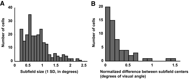
Our model fits allow us to estimate the size and location of two subfields that contribute to the response of V2 neurons. It seems likely that most V2 cells receive input from more than two V1 neurons, in which case our “subunits” may be better thought of as the net effect of a number of V1 inputs. Comparing the properties of our fitted subunits (size and elongation) with reported measurements in V1 might clarify how our subfields related to real V1 neurons. Figure 11A shows a histogram of the subunit SDs. The median value (0.74) is approximately threefold larger than V1 receptive fields, which have been reported to have SD ≃ 0.27 for similar eccentricities (Malone et al. 2007). A similar estimate is produced by measures based on area summation (Cavanaugh et al. 2002). This comparison suggests that our V2 subfields receive input from multiple V1 cells. In many respects, this makes it all the more remarkable that our model, based on the disparity selectivity of only two subunits, explains the data so successfully.

FIG. 11.

Properties of fitted subunits. A: size of subfields (square root of area) in degrees of visual angle. B: distance between the subfield centers, normalized by the mean of the SDs of both subunits. This was calculated along the axis connecting the 2 subfield centers.

We examined the geometrical configuration of the subunits for each cell, to see whether any of the example configurations in Fig. 6 was most representative. We found a striking variety of configurations, with no particular pattern predominating. Most of our quantitative measures of the relationship between the subunits’ geometry revealed no single pattern that was particularly common. The only consistent feature was that the subunits did tend to have substantial spatial overlap. We computed the distance between the centers of the subfields normalized by the size of the subfields (square root of area). More than 85% of the subfields are separated by <0.5SD and only two cells are fit with subfields >1SD apart (Fig. 11B). These results suggest that there may be no systematic organization of the spatial segregation of inputs with different disparity preference; rather cyclopean edge responses may occur as a side effect of the convergence of multiple inputs responding to similar spatial locations without strict regard to disparity tuning. By chance, many of the resulting receptive fields will have “hot spots” for different disparities, which would produce the type of results seen in Bredfeldt and Cumming (2006).

DISCUSSION

Several studies have previously reported that V2 neurons respond to discontinuities in features such as disparity, motion, and orientation in a way not seen in V1. One interpretation of these results is that V2 neurons signal the segmentation of the visual scene (Qiu and von der Heydt 2005). A second possibility is that these signals are based on simple convergence of afferent inputs, which may be useful for scene segmentation, but do not represent its neural basis. Here we put the latter explanation to a quantitative test, by using a simple model that calculates the difference of two V1-like subunit inputs to describe the responses of V2 neurons. This was applied to our data on responses to disparity-defined edges (Bredfeldt and Cumming 2006), which we believe is rich enough to test such models.

We found that models based on a linear combination of the two subunits produced a poor description of the data. Models of this sort predict that for each configuration that produces cyclopean enhancement (responses greater than those produced by uniform disparities), there is a symmetrical configuration that produces suppression (response lower than that produced by uniform disparities). Such suppression was rarely seen in our data. However, this feature of the data was successfully captured if we allowed each subunit a static nonlinearity (squaring) prior to combination. This kind of nonlinearity has been successfully used in many other models of neuronal signal processing (e.g., energy models) and has been widely used in describing the responses of V1 neurons (Adelson and Bergen 1985; Albrecht and Geisler 1991; Anzai et al. 1999; DeAngelis et al. 1993; Heeger 1992; Ohzawa et al. 1997). Indeed its use is so widespread that to use a model with a linear output function for V1 neurons would require some justification.

We were able to provide a good quantitative account of responses to 62 stimulus configurations using only two subunits. However, since our data were gathered using only two disparities, it is not surprising that the responses could be explained in terms of a spatial map of the response difference to the two disparities. Our data would not adequately constrain models that allow more than two subunits if they were all allowed independent disparity tuning. Nonetheless, the fact that this spatial map was well described by the difference of two Gaussians together with the parameters of those Gaussians suggest that it does likely represent the combination of a small number of overlapping V1 receptive fields.

Although our empirical data had 62 statistically independent samples, frequently (e.g., Fig. 5A) many of these samples had very similar response values. Consequently, one might expect a model with <62 parameters to explain the data. The responses in Fig. 5A might be matched with a relatively simple descriptive model (e.g., a Gaussian in polar coordinates, requiring only six parameters). Two such Gaussian functions are required to describe the results in Fig. 5B, but this still requires two fewer parameters than our model; thus the value of the model is not that it describes the data with the fewest number of parameters. Indeed, the linear summation version of our model has only one less parameter, but does not successfully describe the data. Rather, the structure of the model means that there are many patterns of results that it cannot reproduce, which purely descriptive functions could replicate. For example, two distinct regions of cyclopean enhancement, at orientations 90° apart, cannot be reproduced in our model. If one region of enhancement is produced by a vertical edge, for example, any other distinct region of enhancement must occur for a vertical edge with the opposite disparity sign. We confirmed this by generating synthetic data with two regions of enhancement at different orientations and attempting to fit them. The fits never produced discrete regions of enhancement for different orientations. Our model succeeds because this pattern was not seen in the empirical data. Similarly, even when our model responds to vertical edges of both disparity signs, the enhancement occurs at different edge locations (see Fig. 6B). The explanation for this property can be seen by examining the right side of Fig. 1F. This shows two configurations that produce enhancement. In each case, each subunit has the majority of its area covered by its preferred disparity. If one simply swaps the disparities then each subunit must be predominantly covered by its less preferred disparity, a configuration that will not produce enhancement. As discussed in Bredfeldt and Cumming (2006), this is also not seen in the empirical data. In these cases, the success of our model shows that when responses to both signs of disparity edge occur, they are better described by a simple summation than as responses that are invariant with respect to disparity.

These results show that the simple convergence of inputs from a small number of V1 neurons onto a V2 neuron can explain responses to disparity-defined edges. Although this is not evidence against models that propose a more complex feature integration (Craft et al. 2007; Zhaoping 2005), it does indicate the need for more quantitative data to distinguish these two different possibilities. The same principle may apply to other responses observed in V2 that identify feature discontinuities. Ito and Komatsu (2004) reported responses to angles defined by two lines. They concluded that a simple linear summation of responses could not account for the observed responses. We also found that linear summation could not explain responses to disparity-defined edges. Importantly, incorporating a simple output exponent in the responses of our V1-like subunits was sufficient to produce a good description of our data. A model with a similar structure may be sufficient to describe responses to angle stimuli, as was also pointed out by Boynton and Hegde (2004). Whether such a simple model is successful across the whole range of responses observed in the population would require a quantitative study, of the type we report here for disparity-defined edges. Similarly, it seems likely that models of this sort could explain selectivity for motion-defined borders (Marcar et al. 2000). One interesting prediction of our simple model may differentiate simple bottom-up models from more complex feature integration. Reversing the contrast of one eye's image (“anticorrelation”) inverts disparity-selective responses in V1 (Cumming and Parker 1997). Thus in our model anticorrelation will reverse the sign of cyclopean edge effects, but the model will still respond selectively to the cyclopean edge. Note that no additional simulations are required to demonstrate this. The model responses depend only on the responses of each subunit to the two disparities (S1_d1, S1_d2, S2_d1, S2_d2 in Eqs. 1–3), and so the simulation behaves in exactly the same way if these are elicited by anticorrelated stimuli. However, disparity-defined edges in anticorrelated stimuli are not visible to observers (Cumming et al. 1998). Thus neurons that represent the perceptual experience of figure–ground segregation should cease to respond. Interestingly the same model structure can be used to explain the relatively weak responses elicited by anticorrelated stimuli with uniform disparity (Haefner and Cumming 2008; Tanabe and Cumming 2008). This would allow a single model to explain both the responses to anticorrelated stimuli and the responses to cyclopean edges, even if the responses to anticorrelated stimuli were weaker in V2 than in V1 (although current data suggest that the responses are similar; Tanabe and Cumming 2008).

The simple convergence of V1 outputs in our model is reminiscent of Hubel and Wiesel's model for producing V1 simple cells from lateral geniculate nucleus (LGN) inputs (for review, see Ferster and Miller 2000). Although most implementations of this model assume that LGN inputs to V1 are systematically organized to create simple cell receptive fields, some recent studies have suggested that the observed responses could be explained by haphazard wiring (Ringach 2004). The properties of the subunits in our model suggest that haphazard wiring could readily account for the generation of orientation-selective responses to disparity-defined edges in V2. Thus it is possible that at least some of the apparently complex stimulus response properties found in V2 cells may be an accident of unorganized convergence, rather than arising from a more complex underlying organizational principle.

GRANTS

This work was supported by the Intramural Research Program of the National Institutes of Health, National Eye Institute, and by Royal Society University Research Fellowship Grant UF041260 awarded to J.C.A. Read.

REFERENCES

- Adelson and Bergen 1985.Adelson EH, Bergen JR. Spatiotemporal energy models for the perception of motion. J Opt Soc Am A 2: 284–299, 1985. [DOI] [PubMed] [Google Scholar]
- Albrecht and Geisler 1991.Albrecht DG, Geisler WS. Motion selectivity and the contrast-response function of simple cells in the visual cortex. Vis Neurosci 7: 531–546, 1991. [DOI] [PubMed] [Google Scholar]
- Anzai et al. 1999.Anzai A, Ohzawa I, Freeman RD. Neural mechanisms for processing binocular information. I. Simple cells. J Neurophysiol 82: 891–908, 1999. [DOI] [PubMed] [Google Scholar]
- Boynton and Hegde 2004.Boynton GM, Hegde J. Visual cortex: the continuing puzzle of area V2. Curr Biol 14: R523–R524, 2004. [DOI] [PubMed] [Google Scholar]
- Bredfeldt and Cumming 2006.Bredfeldt CE, Cumming BG. A simple account of cyclopean edge responses in macaque V2. J Neurosci 26: 7581–7596, 2006. [DOI] [PMC free article] [PubMed] [Google Scholar]
- Cavanaugh et al. 2002.Cavanaugh JR, Bair W, Movshon JA. Nature and interaction of signals from the receptive field center and surround in macaque V1 neurons. J Neurophysiol 88: 2530–2546, 2002. [DOI] [PubMed] [Google Scholar]
- Craft et al. 2007.Craft E, Schutze H, Niebur E, von der Heydt R. A neural model of figure–ground organization. J Neurophysiol 97: 4310–4326, 2007. [DOI] [PubMed] [Google Scholar]
- Cumming and Parker 2007.Cumming BGC, Parker AJ. Responses of primary visual cortical neurons to binocular disparity without depth perception. Nature 389: 280–283, 2007. [DOI] [PubMed] [Google Scholar]
- DeAngelis et al. 1993.DeAngelis GC, Ohzawa I, Freeman RD. Spatiotemporal organization of simple-cell receptive fields in the cat's striate cortex. II. Linearity of temporal and spatial summation. J Neurophysiol 69: 1118–1135, 1993. [DOI] [PubMed] [Google Scholar]
- Ferster and Miller 2000.Ferster D, Miller KD. Neural mechanisms of orientation selectivity in the visual cortex. Annu Rev Neurosci 23: 441–471, 2000. [DOI] [PubMed] [Google Scholar]
- Haefner and Cumming 2008.Haefner RM, Cumming BG. Adaptation to natural binocular disparities in primate V1 explained by a generalized energy model. Neuron 57: 147–158, 2008. [DOI] [PMC free article] [PubMed] [Google Scholar]
- Haynes et al. 2004.Haynes JD, Lotto RB, Rees G. Responses of human visual cortex to uniform surfaces. Proc Natl Acad Sci USA 101: 4286–4291, 2004. [DOI] [PMC free article] [PubMed] [Google Scholar]
- Heeger 1992.Heeger DJ Half-squaring in responses of cat striate cells. Vis Neurosci 9: 427–443, 1992. [DOI] [PubMed] [Google Scholar]
- Hegde and Van Essen 2000.Hegde J, Van Essen DC. Selectivity for complex shapes in primate visual area V2. J Neurosci 20: RC61, 2000. [DOI] [PMC free article] [PubMed] [Google Scholar]
- Hubel and Wiesel 1962.Hubel DH, Wiesel TN. Receptive fields, binocular interaction and functional architecture in the cat's visual cortex. J Physiol 160: 106–154, 1962. [DOI] [PMC free article] [PubMed] [Google Scholar]
- Ito and Komatsu 2004.Ito M, Komatsu H. Representation of angles embedded within contour stimuli in area V2 of macaque monkeys. J Neurosci 24: 3313–3324, 2004. [DOI] [PMC free article] [PubMed] [Google Scholar]
- Malone et al. 2007.Malone BJ, Kumar VR, Ringach DL. Dynamics of receptive field size in primary visual cortex. J Neurophysiol 97: 407–414, 2007. [DOI] [PubMed] [Google Scholar]
- Marcar et al. 2000.Marcar VL, Raiguel SE, Xiao D, Orban GA. Processing of kinetically defined boundaries in areas V1 and V2 of the macaque monkey. J Neurophysiol 84: 2786–2798, 2000. [DOI] [PubMed] [Google Scholar]
- Nienborg et al. 2004.Nienborg H, Bridge H, Parker AJ, Cumming BG. Receptive field size in V1 neurons limits acuity for perceiving disparity modulation. J Neurosci 24: 2065–2076, 2004. [DOI] [PMC free article] [PubMed] [Google Scholar]
- Ohzawa et al. 1997.Ohzawa I, DeAngelis GC, Freeman RD. Encoding of binocular disparity by complex cells in the cat's visual cortex. J Neurophysiol 77: 2879–2909, 1997. [DOI] [PubMed] [Google Scholar]
- Prince et al. 2002.Prince SJ, Pointon AD, Cumming BG, Parker AJ. Quantitative analysis of the responses of V1 neurons to horizontal disparity in dynamic random-dot stereograms. J Neurophysiol 87: 191–208, 2002. [DOI] [PubMed] [Google Scholar]
- Qiu and von der Heydt 2005.Qiu FT, von der Heydt R. Figure and ground in the visual cortex: V2 combines stereoscopic cues with gestalt rules. Neuron 47: 155–166, 2005. [DOI] [PMC free article] [PubMed] [Google Scholar]
- Read and Cumming 2003.Read JCA, Cumming BG. Measuring VI receptive fields despite eye movements in awake animals. J Neurophysiol 90: 946–960, 2003. [DOI] [PMC free article] [PubMed] [Google Scholar]
- Ringach 2004.Ringach DL Haphazard wiring of simple receptive fields and orientation columns in visual cortex. J Neurophysiol 92: 468–476, 2004. [DOI] [PubMed] [Google Scholar]
- Tanabe and Cumming 2008.Tanabe S, Cumming BG. Mechanisms underlying the transformation of disparity signals from V1 to V2 in the macaque, J Neurosci 28: 11304–11314, 2008. [DOI] [PMC free article] [PubMed] [Google Scholar]
- von der Heydt et al. 2000.von der Heydt R, Zhou H, Friedman HS. Representation of stereoscopic edges in monkey visual cortex. Vision Res 40: 1955–1967, 2000. [DOI] [PubMed] [Google Scholar]
- Zhaoping 2005.Zhaoping L Border ownership from intracortical interactions in visual area V2. Neuron 47: 143–153, 2005. [DOI] [PubMed] [Google Scholar]
- Zhou et al. 2000.Zhou H, Friedman HS, von der Heydt R. Coding of border ownership in monkey visual cortex. J Neurosci 20: 6594–6611, 2000. [DOI] [PMC free article] [PubMed] [Google Scholar]