Body odour of monozygotic human twins: a common pattern of odorant carboxylic acids released by a bacterial aminoacylase from axilla secretions contributing to an inherited body odour type

Abstract

It is currently not fully established whether human individuals have a genetically determined, individual-specific body odour. Volatile carboxylic acids are a key class of known human body odorants. They are released from glutamine conjugates secreted in axillary skin by a specific N_α-acyl-glutamine-aminoacylase present in skin bacteria. Here, we report a quantitative investigation of these odorant acids in 12 pairs of monozygotic twins. Axilla secretions were sampled twice and treated with the N_α-acyl-glutamine-aminoacylase. The released acids were analysed as their methyl esters with comprehensive two-dimensional gas chromatography and time-of-flight mass spectrometry detection. The pattern of the analytes was compared with distance analysis. The distance was lowest between samples of the right and the left axilla taken on the same day from the same individual. It was clearly greater if the same subject was sampled on different days, but this intra-individual distance between samples was only slightly lower than the distance between samples taken from two monozygotic twins. A much greater distance was observed when comparing unrelated individuals. By applying cluster and principal component analyses, a clear clustering of samples taken from one pair of monozygotic twins was also confirmed. In conclusion, the specific pattern of precursors for volatile carboxylic acids is subject to a day-to-day variation, but there is a strong genetic contribution. Therefore, humans have a genetically determined body odour type that is at least partly composed of these odorant acids.

1. Introduction

A well-known capability of canines is their ability to track human subjects based on their odour. This implicates individual-specific body odour types in humans. Furthermore, it has also been shown that dogs have difficulties in discriminating between monozygotic twins (Hepper 1988), indicating that body odour is a genetically fixed trait. A recent study (Roberts et al. 2005) showed that human subjects can discriminate between the odours of dizygotic twins much better then between the odours of monozygotic twins. These observations were all made at a sensorial or behavioural level, and the compounds that result in genetically fixed human body odours and the biochemical mechanisms leading to the formation of this unique body odour have not been characterized in these studies.

Sommerville et al. (1994) used gas chromatography (GC) to recognize patterns of volatile compounds in a few pairs of twins, but the flame ionization detector used could not lead to identification of the volatile compounds. A recent study by Penn et al. (2007) used GC–MS to investigate whether there is a stable pattern of volatiles emitted by human subjects and to identify the relevant chemicals discriminating sex and individuals. However, most of the chemicals found in that study as marker compounds discriminating individuals or the two sexes are commonly used fragrance molecules, sunscreens and cosmetic ingredients. Thus, for example, the synthetic sunscreen Parsol MCX (2-ethyl-hexyl-4-methoxycinnamate) was among the seven analytes proposed to be female-specific odorants. Therefore, the results rather reflected personal grooming habits of individuals than a physiologically determined odour type. Finally, Curran et al. (2005) investigated the volatiles in the headspace of human subjects. They found mainly common straight chain fatty acids, fatty aldehydes and alkanes differentiating individuals. These two detailed analytical studies had the same limitations, inasmuch as they defined ‘odour’ as ‘any volatile molecule detectable with a gas chromatograph’. A socially relevant body odour type, however, is the odour perceived by the conspecifics, and thus it should be ensured that the observed individual typical chemicals indeed (i) are coming from human physiology and (ii) are perceivable by the human nose.

Several studies have addressed in detail the chemical nature of human body odorants secreted in the axilla. Early studies had found the two odoriferous steroids 5α-androst-16-en-3-one and 5α-androst-16-en-3α-ol (Brooksbank et al. 1974; Claus & Alsing 1976). A detailed analysis of the chemical composition of axillary odour was later presented by Zeng et al. (1991). They reported that (E)-3-methyl-2-hexenoic acid is the key odour component but they also found several other carboxylic acids. In our previous work (Natsch et al. 2006), we had identified a series of 26 different carboxylic acids in axilla secretions, which are secreted as N_α-acyl-glutamine-conjugates and which are released from these conjugates by the enzyme N_α-acyl-glutamine-aminoacylase (N-AGA) isolated from commensal skin bacteria inhabiting the human axilla (Natsch et al. 2003, 2006). We had shown that most of these acids are odorants and that they occur in different ratios on different individuals, but whether these ratios are stable over time and whether they are genetically fixed had not been investigated. Finally, different sulfanylalkanols have been reported by several authors as further odour components in axilla secretions (Hasegawa et al. 2004; Natsch et al. 2004; Troccaz et al. 2004). Interestingly, these specific human body odorants were not detected at all in the analytical population studies summarized above addressing the question of an individual-specific odour type (Curran et al. 2005; Penn et al. 2007). Thus, there is a gap between these analytical population studies on the one hand and the analytical studies that had identified specific human body odorants on the other hand.

Genetically determined body odour types in animals (and in humans) have mostly been discussed in relation to odour-dependent mate selection. In mice, odour-dependent mate selection is a well-established penomenon and it leads to couples with dissimilar alleles in the major histocompatibility complex (MHC) loci, thus maximizing the frequency of MHC heterozygotes in the offspring and preventing inbreeding (Yamazaki et al. 1976; Yamaguchi et al. 1981). Several studies with humans judging the body odours on worn T-shirts also point to a preference for body odours of MHC-dissimilar persons (Wedekind et al. 1995; Wedekind & Füri 1997). These studies indicated that in mice and men, individuals have a distinct body odour type that is (i) genetically determined and (ii) more specifically determined at least partly by MHC alleles, although the underlying mechanism is unknown.

Comprehensive two-dimensional gas chromatography (GC×GC) with time-of-flight mass spectrometry (ToF-MS) detection is one of the most powerful separation and identification tools for volatile organic compounds. GC×GC provides an increased separation power compared with one-dimensional GC and has proved useful for complex sample analysis in recent years (e.g. Marriott & Shellie 2002; Beens & Brinkman 2005; Adahchour et al. 2006a). Two columns with different selectivity are connected in series, and a modulator installed in between provides for a pulsed transfer of the whole eluate from the first dimension (¹D) column to the second dimension (²D) column. The modulation time, i.e. the ²D chromatogram time, should be smaller than a typical ¹D GC peak width for proper chromatographic resolution and peak integration. As a consequence, a given analyte will be split into several ²D chromatographic peaks called subpeaks that are eluting in consecutive ²D chromatograms. With dedicated software, two- and three-dimensional views of the linear chromatographic raw data are generated. Algorithms for mass spectral deconvolution can locate and identify analytes that are still co-eluting in GC×GC if a ToF-MS detector is used. For the final evaluation, efficient software tools are necessary in order to find and integrate chromatographic peaks, to correctly merge subpeaks belonging together and thereby to ensure reliable quantifications. Data evaluation can best be automated with user-defined processing methods that are based on both retention times and mass spectra of the relevant analytes.

Here, we try to make the connection between (i) the studies that had addressed the chemical nature of human body odours and (ii) the studies that had shown, at the sensorial level, that there is a genetically determined body odour in humans. We therefore report a new GC×GC–ToF-MS method to quantitatively monitor the pattern of the odorant acids. This method was applied in an analytical study on 12 pairs of monozygotic twins, testing the hypothesis that a specific pattern of these acids forms part of a genetically fixed body odour type in humans and thus determine a ‘chemical fingerprint’ of the individuals.

2. Experimental procedures

2.1 General

All reagents and solvents were purchased from Fluka if not otherwise noted. The synthesis of reference compounds has been described before (Natsch et al. 2003, 2006).

2.2 Subjects and study set-up

Fourteen pairs of monozygotic twins were recruited. Participation was voluntary, subjects were informed about the goals of the study and they were compensated for their participation. The study population and sample list are summarized in table 1. Two female pairs had to be excluded from final analysis, since the concentration of volatiles in one of the individuals was very low and below the detection limit for most analytes. Each subject was sampled twice on different days with at least a one-week interval between the two sampling days. The samples from the right and left axillae were analysed individually.

Table 1.

Study population and sample list.

individual	age	sex	sampling 1, right	sampling 1, left	sampling 2, right	sampling 2, left
2a	52	M	2.2a	2.8	1.0	1.0
2b	52	M	1.7	1.7	2.0	1.0
3a	39	F	3.0	3.0	3.0	3.0
3b	39	F	3.0	3.0	1.0	3.0
4a	18	M	1.0	2.6	2.3	2.5
4b	18	M	4.6	4.3	3.3	4.0
5a	45	F	1.0	1.0	1.0	1.0
5b	45	F	1.0	1.0	1.0	1.0
6a	53	M	2.9	2.1	1.0	1.0
6b	53	M	2.7	2.3	4.1	2.7
7a	26	M	1.0	1.0	1.0	1.0
7b	26	M	1.0	1.0	1.0	1.0
8a	28	M	1.8	1.0	1.0	1.0
8b	28	M	1.0	1.0	1.0	1.0
9a	22	F	1.0	1.0	1.0	sample lost
9b	22	F	1.0	1.0	1.0	1.0
10a	45	F	1.0	1.0	1.0	1.0
10b	45	F	1.0	1.0	1.0	1.0
11a	32	F	3.0	2.5	1.5	3.0
11b	32	F	1.9	1.8	1.0	2.3
12a	35	F	1.0	1.0	1.0	1.0
12b	35	F	1.0	1.0	1.0	1.0
13a	18	F	1.0	1.0	1.0	1.0
13b	18	F	1.0	1.0	1.0	1.0

^aIndicates dilution factor.

2.3 Collection of axilla secretions and treatment with the recombinant N-AGA

Axilla secretions of individual donors were sampled on cotton pads fixed in the axilla during 45–60 min of physical exercise. Individual pads were suspended in 25 ml of 30 per cent EtOH in H₂O immediately after collection to avoid any bacterial metabolism and they were sent to the analysis laboratory where they were frozen at −80°C until analysis, with a maximal storage time for the samples of two weeks. Pads were removed from the sampling solution and the Gln-conjugate 5-amino-2-(2-methylundecanamido)-5-oxopentanoic acid was added as internal standard (ISTD1, final concentration 0.8 μM). The liquid phase was extracted once with 5 ml hexane, and the hexane fraction was saved. The aqueous phase was lyophilized for 16 hours and re-suspended in 0.7 ml H₂O. A 0.4 ml sample of this concentrated aqueous extract was treated with a large excess of the recombinant enzyme N-AGA (4.5 μg per sample, produced and purified as described before; Natsch et al. 2003) to ensure complete hydrolysis of the Gln conjugates. After 4 hours incubation at 36° C, 30 μl of 1 M HCl and 50 mg NaCl were added and the sample was extracted with 100 μl methyl-tert-butyl-ether (MTBE). The organic phase (80 μl) was transferred to a GC vial, 5 μl of a 2 M solution of (trimethylsilyl)-diazomethane (Fluka, Buchs, Switzerland) and 18 μl of methanol containing 0.5 mM ethyl-caprinate as second internal standard (ISTD2) were added, and the sample was heated to 40°C for 30 min to form the methyl esters of the enzymatically released acids.

2.4 GC×GC–ToF-MS analysis of axilla secretions

2.4.1 Instrumentation, separation and detection

A LECO Pegasus 4D GC×GC–ToF-MS system (LECO, St. Joseph, MI, USA) was used, consisting of a 6890N (Agilent Technologies, Palo Alto, CA, USA) gas chromatograph equipped with split/splitless injector, a dual stage, four-jet cryogenic modulator (licensed from Zoex), a second dimension column oven and a Pegasus III time-of-flight mass spectrometer (LECO). Sample volumes of 1 μl were injected in the splitless mode at an injector temperature of 230°C using a Gerstel MPS2 autosampler (Gerstel, Muelheim an der Ruhr, Germany) equipped with a cooling tray kept at 10°C. Helium was employed as carrier gas at a constant flow of 1 ml min⁻¹. A capillary column of 60 m length × 0.25 mm i.d. coated with 0.25 μm of VF-5MS (5% phenyl–95% dimethyl-polysiloxane) was used for the first dimension. The second dimension was a 2 m length × 0.1 mm i.d. capillary column with a 0.10 μm thick film CP-WAX 52 CB (polyethylene glycol, both from Varian, Palo Alto, CA, USA). Separations were effected using the following temperature programme: 30°C, isothermal for 5 min, then 10°C min⁻¹ to 120°C, 2°C min⁻¹ to 260°C, isothermal for 5 min. The separate second dimension oven was set to a temperature constantly 5°C higher than the first dimension column oven. The modulation time was 7 s. The modulator housing was kept at 20°C above the first dimension oven temperature. Liquid nitrogen was used for cooling the two cold jets. The transfer line and ion source temperatures were kept at 230°C. The ToF-MS was operated at a storage rate of 200 Hz, using a mass range of m/z 25–350 and in electron ionization mode at 70 eV. The target analytes were identified by reference compound injection and/or spectral matching to a library database and/or homologous series position on the separation plane and interpretation of their mass spectra (see table S1 in the electronic supplementary material).

2.5 Processing methods

The study design required the finding, correct combining, identifying and quantifying of 7410 subpeaks (95 samples×26 analytes, with an assumed three modulations per ¹D peak; 24 endogenous analytes and two internal standards). Therefore, much emphasis was placed on the development of a reliable automatic data processing (DP) routine. The LECO ChromaTOF v. 3.25 software was used for data treatment. Each raw file was processed with the same set of five different DP methods (1–5). Every method was optimized for one or a group of target analytes with similar peak widths using the parameters summarized in table 2. Based on these parameters, the algorithm was capable of finding and combining subpeaks. In a next step, the software had to identify and quantify the target analytes. For this purpose, a DP method accessed a separate reference table (table 3) with the following target analyte information stored: full scan reference spectrum; expected first and second dimension retention time windows; required minimum signal to noise (S/N); required match factor for the comparison of the measured to the saved full scan reference spectrum; and the quantification m/z ion. The analyte identification criteria in the reference table were kept as strict as possible in order to avoid wrong assignments. As a consequence, approximately 6 per cent of the peaks, all not found by the algorithm, had to be checked and added manually. After this manual peak integration of the missing peaks, for each of the 24 endogenous analytes, a peak area could be integrated in all samples, which resulted in a data matrix without any missing value. Each DP method created a csv file with the identified and integrated analyte information. These 380 csv files were imported into Microsoft Access (Redmond, USA) by a macro.

Table 2.

Summary of DP parameters.

	DP method (analyte concentration level/analyte polarity)
DP parameters	1 (low/low)	3 (low/middle)	4 (low/high)	2 (high/low)	5 (very high/low)
expected 1D peak width (s)	14	14	14	42	49
expected 2D peak width (s)	0.100	0.200	0.400	0.400	0.600
2D S/N	3	1	1	3	50
masses m/z	25–27, 29–31, 33–43, 45–350				146
number of apexing masses	2	2	1	2	1
Match required to combine subpeaks	750	750	750	750	500
allowed 2D RT shift for combining subpeaks±(s)	0.010	0.030	0.050	0.200	0.300

Table 3.

Overview of reference table settings.

analyte	DPa method	Quan m/z	expected 1D RT window (s)	expected 2D RT window (s)	required match factor
A2	5	146	1558±21	2.780±0.848	700
A3	1	117	1775±0	2.953±0.289	900
A4	1	117	2048±0	3.115±0.322	900
B1	3	103	1691±0	3.475±0.405	900
B2	3	103	1929±7	3.665±0.435	900
B3	3	103	2209±0	3.775±0.449	900
B4	3	103	2524±0	3.795±0.442	900
B5	3	103	2846±0	3.798±0.438	900
B6	3	103	3070±0	3.735±0.435	800
C1	3	103	1509±7	3.403±0.401	900
C2	3	103	1740±7	3.765±0.465	850
C3	3	103	2020±14	3.995±0.465	900
C4	3	103	2657±0	4.110±0.502	900
E1	2	74	1481±0	2.093±0.102	900
E2	1	95	1411±0	1.940±0.090	900
F1	1	96	1873±0	2.290±0.150	900
F2	1	96	1831±7	2.258±0.138	900
F4	1	96	2146±7	2.440±0.157	900
H1	4	74	2447±14	6.540±1.030	750
H2	4	74	2776±14	6.058±0.955	750
ISTD1	2	88	2622±0	2.215±0.120	850
ISTD2	2	88	2419±0	2.210±0.120	900
Ph	3	91	1817±7	3.713±0.461	850
Z1	1	87	2027±7	2.138±0.116	900
Z3	1	87	1943±0	2.093±0.109	900
Z5	4	99	2797±7	5.101±0.727	850

^aDP, data processing; Quan, quantitation ion; ¹D, first dimension; ²D, second dimension; RT, retention time.

2.6 Quantification

Subpeaks of the analytes were integrated on their extracted mass chromatograms. Quantification ions with both high selectivity and intensity (30–100% relative abundance in their respective mass spectra) were selected for 22 endogenous analytes. Two further analytes (E1 and A2) occurred in concentrations up to two or three orders of magnitude higher than the other analytes. Therefore, ions with low intensity had to be chosen for E1 and A2 because the intense mass signals would have saturated the detector. As an example, for A2 the m/z 146 was selected (corresponds to the ¹³C isotope signal of the methyl radical loss m/z 145) which had a relative intensity of 0.3 per cent in the mass spectrum but still a strong detector response and was a rather unique ion to A2. There were 33 samples that were outside of the linear range and which therefore were diluted with MTBE and analysed again; these dilutions are indicated in table 1.

2.7 Method validation

Validation data are summarized in table S1 in the electronic supplementary materials. The linearity of the method was tested with three calibration experiments on different days and at 13 concentration levels with single measurements. Six reference compounds A2, B2, C3, E1, F1 and F4 (for structures, see table 4) belonging to different chemical classes were chosen. The calibration curves were linear within three (A2, B2, E1) or two (C3, F1, F4) orders of magnitude with correlation coefficients (R²) ranging from 0.998 to 0.996. Only few samples of the study had sporadic analyte concentrations out of the linear range or in a range not tested. Limit of detection at a S/N of three on the quantification ion mass chromatogram was approximately 10–30 pg μl⁻¹ (except A2 that was deliberately higher). The relative standard deviation (RSD%, n=3) of the peak area was determined for all calibration analytes and every concentration level above limit of quantification (S/N=5). The mean of these RSD% was 10–15 per cent for any given analyte. This was an acceptable variation taking into account the complexity (subpeaks) of the raw data and the fully automated processing and turned out to be similar or somewhat bigger than the one reported in the review of Adahchour et al. (2006b) for six GC×GC–ToF-MS methods.

Table 4.

Chemical identification of the derivatized key analytes released by N-AGA and results of nested ANOVA analysis from all the 95 samples.

			% variance attributed to different hierarchical levels according to nested ANOVA analysis
identifiera	structure	name	sex	pair	individual	sampling day	right/left
A2		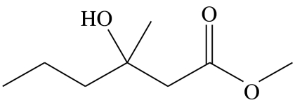3-hydroxy-3-methylhexanoic acid-methyl-ester	0.0	67.9	6.2	13.3	12.6
A3		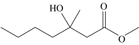3-hydroxy-3-methylheptanoic acid-methyl-ester	9.9	47.3	3.2	11.3	28.3
A4		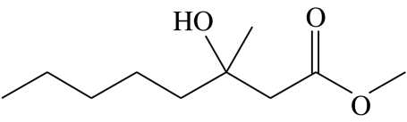3-hydroxy-3-methyloctanoic acid-methyl-ester	10.7	62.7	16.6	2.0	8.1
B1		3-hydroxy-4-methylhexanoic acid-methyl-ester	48.3	35.3	0.0	10.8	5.7
B2		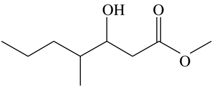3-hydroxy-4-methylheptanoic acid-methyl-ester	27.6	54.6	2.5	9.8	5.6
B3		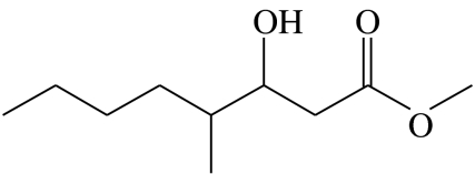3-hydroxy-4-methyloctanoic acid-methyl-ester	0.0	79.7	9.5	8.2	2.6
B4		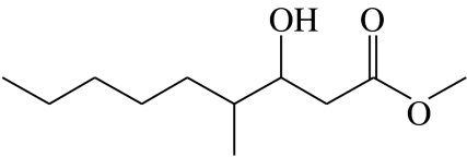3-hydroxy-4-methylnonanoic acid-methyl-ester	0.0	54.8	26.4	16.5	2.3
B5		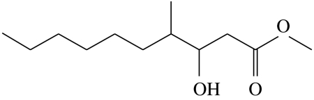3-hydroxy-4-methyldecanoic acid-methyl-ester	0.0	45.9	25.0	22.3	6.9
B6	unknown		3.0	41.5	34.1	16.0	5.4
C1		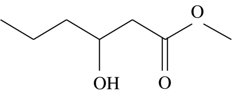3-hydroxyhexanoic acid-methyl-ester	5.2	40.0	5.7	10.5	38.6
C2		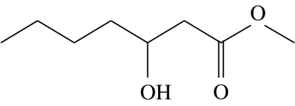3-hydroxyheptanoic acid-methyl-ester	24.9	18.9	0.0	30.6	25.6
C3		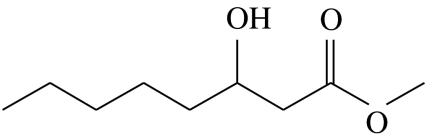3-hydroxyoctanoic acid-methyl-ester	0.0	70.8	5.2	21.9	4.2
C4		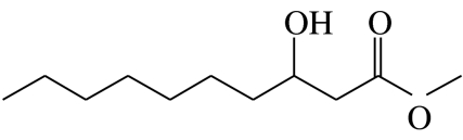3-hydroxydecanoic acid-methyl-ester	0.0	56.9	0.0	35.8	7.4
E1		(E)-3-methylhex-2-enoic acid-methyl-ester	12.8	59.8	2.6	20.8	4.1
E2		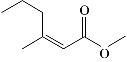(Z)-3-methylhex-2-enoic acid-methyl-ester	0.0	67.7	11.1	9.5	11.7
F1		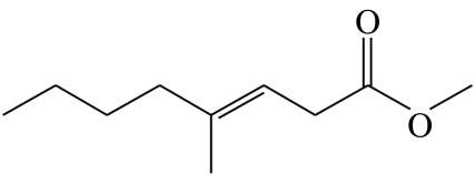(E)-4-methyloct-3-enoic acid-methyl-ester	0.0	78.9	11.6	4.0	5.5
F2		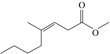(Z)-4-methyloct-3-enoic acid-methyl-ester	0.0	78.4	10.8	5.0	5.8
F4		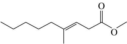(E)-4-methylnon-3-enoic acid-methyl-ester	0.0	53.9	32.4	9.8	3.9
H1		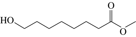8-hydroxyoctanoic acid-methyl-ester	6.6	28.6	0.0	26.3	38.5
H2		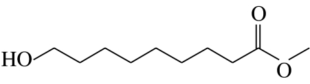9-hydroxynonanoic acid-methyl-ester	0.0	1.0	0.0	0.0	99.0
Ph		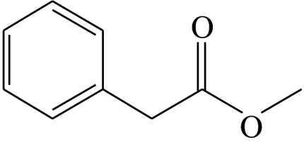phenylacetic acid-methyl-ester	40.9	27.6	15.0	13.0	3.5
Z1		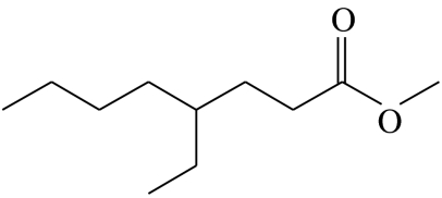4-ethyloctanoic acid-methyl-ester	26.0	14.6	55.5	1.9	2.1
Z3		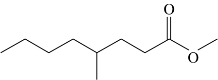4-methyloctanoic acid-methyl-ester; hypothetical structure not verified by synthetic sample	9.5	50.8	34.1	1.5	4.0
Z5		δ-decalactone	14.2	48.4	12.8	11.2	13.4
	average values for nested ANOVA		10.4	51.5	13.9	13.6	10.71

^aListed are all compounds that were at least 20-fold enhanced by enzyme treatment in a pooled sample and that are present in all samples.

2.8 Evaluation of results

The consolidated GC×GC–ToF-MS analyses resulted in a matrix of 95 samples, with peak areas for 24 endogenous analytes per sample. First, a normalization step as used by Xu et al. (2007) was performed, since the amount of sweat in the different samples is difficult to control (different intensity of physical exercise and different transfer of sweat from skin to the pad): each analyte in a sample was divided by the sum of all evaluated analytes for the given sample thus normalizing the sum of all evaluated analytes in a sample to 1. All the data analysis was then performed with these normalized data. As the presence of more intense peaks could distort the data when performing this normalization step, often a square root or log transformation is applied to such datasets prior to the normalization step. All the calculations were also performed with these alternative approaches (either square root or log transformation prior to normalization). Very similar results were obtained with these different calculations, and thus all the data shown are based on the direct normalization of the data without further data transformation.

The distance between two samples was calculated by forming, for each analyte, the ratio of the normalized peak areas between two samples, then taking the logarithm of this ratio, taking the absolute value of this logarithm, and then summing up these absolute values for all analytes and dividing by the number of analytes to obtain a symmetrical distance measure according to

$$\text{distance}=\frac{\sum _{n=1}^m\left|\text{log}\frac{X_n}{Y_n}\right|}{m},$$ (2.1)

where X and Y are the two samples; m is the number of analytes; and X_n and Y_n are the normalized peak areas for a given analyte n in the two samples.

This distance measure based on ratios of peak intensities between samples does correct for the fact that the different analytes have different relative abundances and different scales (i.e. different m/z ions were used for their integration). Also this distance measure is symmetrical, thus the distance of sample X to Y is identical to the distance of Y to X. By taking absolute values of the logarithm, there are no negative values.

Alternatively, the normalized Euclidean distance was calculated according to

$$\text{normalized}\text{Euclidean}\text{distance}=\sqrt{\sum _{n=1}^m{{\displaystyle \left(\frac{(X_n-Y_n)}{s_n}\right)}}^2},$$ (2.2)

where X and Y are the two samples; m is the number of analytes; X_n and Y_n are the normalized peak areas of analyte n in the two samples; and s_n is the measured standard deviation for the peak n over all samples.

The data in the main text were calculated with the distance according to equation (2.1). Similar results were obtained with the normalized Euclidean distance and results of this later analysis are included in the electronic supplementary material.

Based on the above equations, a distance matrix with all possible comparisons between individual samples was calculated. The distances between samples (i) from the same individual and on the same sampling day, (ii) from the same individual on different days, (iii) from two twins and finally (iv) the distance between samples originating from unrelated individuals were then compared. In addition, the distance matrix was transformed to ranks, assigning to each sample 94 ranks based on the distance it has to all the other samples.

Cluster analysis with the complete linkage algorithm based on the distance matrix calculated according to equation (2.1) was performed with Matlab (Statistics Toolbox v. 6.0, The MathWorks, Inc., 3 Apple Hill Drive, Natick, MA 01760-2098, USA). All other statistical procedures were done with the Minitab statistical software (Minitab Inc., v. 15.1.1.0, Coventry, UK). Principal component analysis (PCA) was performed based on the correlation matrix. Nested ANOVA analysis on the normalized data was used to evaluate the variance of the single analytes due to the hierarchical design of the study (with two sexes, different pairs, individuals within the pairs, different sampling days within the individuals and finally left versus right sampling on the same day). Nested ANOVA allows assigning the variance to the different hierarchical levels in the sampling regimen.

3. Results

3.1 Identification and selection of target analytes in the odorant fraction of hydrolysed sweat

As observed previously (Shelley et al. 1953; Troccaz et al. 2004; Natsch et al. 2006), both the concentrated hexane fraction and the concentrated aqueous fraction of sweat samples obtained by physical exercise had only a faint odour, which is in line with the well-established notion that odour is only released by bacterial action (Shelley et al. 1953). Within a pooled hexane fraction, a large number of components were identified by routine database comparison, but the 25 most abundant peaks appear either to be exogenous (especially fragrance components, emollients used in cosmetics, plasticizers and antioxidants) or they are simple fatty acids (C14–C18, saturated and unsaturated) and squalene, compounds generally present in the skin. Finally, odourless hydrocarbons are also predominant in this fraction (data not shown). Owing to the low odour of the hexane fractions, these compounds do not appear to contribute significantly to body odour and the further analysis thus focused on the aqueous phase. For a first analytical inventory, a pool with aliquots of all aqueous samples was split in two and one half was treated with the specific N_α-acyl-glutamine-aminoacylase whereas the other was left untreated. The untreated sample had only a faint, acidic odour, whereas the pooled, enzyme-treated sample developed a very pungent, typical axilla odour as observed before (Natsch et al. 2006). The two samples were compared after methyl ester formation by comprehensive GC×GC–ToF-MS. They contained a range of methyl esters in common, but due to the faint odour of the untreated sample, we focused on all peaks that were at least 20-fold increased in the enzyme-treated sample and therefore appeared to contribute to the very strong odour developing in this sample. In total, the list of these analytes comprised 35 compounds. Many of them had been found before (Zeng et al. 1991; Natsch et al. 2006) and their odour had been characterized (Zeng et al. 1991; Natsch et al. 2003, 2006; Hasegawa et al. 2004). They primarily comprised methyl esters of series of methyl-branched, unsaturated or hydroxylated acids. Table 4 lists the 24 key compounds, which were above the detection limit in all samples and which did not co-elute with other constituents. Figure 1 shows the GC×GC–ToF-MS three dimensional and the colour plot of the pooled, enzyme-treated sample with the key analytes being labelled. The intensities are given by the sum of the abundances of all ions detected (total ion current, TIC). Figure 2 shows three-dimensional plots of the same chromatographic region for four individual samples obtained from two pairs of twins. Here, the intensities are given by the sum of the abundances of the extracted ions m/z 117, 103, 114, 96 and 150, which are characteristic ions for different target analytes. GC×GC–ToF-MS yielded a much better overview of the constituents in the sample when compared with one-dimensional GC, owing to the chemically meaningful structure of the peak positions across the chromatographic plane and owing to the enormous separation power. Although much effort was spent to produce clean sweat GC samples, they were still complex with a variable biological matrix, and in one-dimensional GC many co-elutions were observed, especially in the low concentration range (see Natsch et al. 2006) where most of the sweat odour constituents occurred. Thus, the discovery of compounds, identification of unknowns (especially homologues) and comparison of samples were facilitated by the novel GC×GC method.

Figure 1.

GC×GC–ToF-MS total ion current (TIC) plots for the pooled sample, treated with N-AGA and derivatized with (trimethylsilyl)-diazomethane: (a) three-dimensional plot and (b) colour plot. Labels identify the key analytes and black dots mark peak apexes. The relative abundance of analyte A2 is 100% and the colour gradient goes from 0 to 5% (blue to red).

Figure 2.

Individual GC×GC–ToF-MS three-dimensional plots from pairs 4 and 8. Chromatograms for four individuals (a) 4a, (c) 4b, (b) 8a and (d) 8b are shown. GC peak intensities are the sums of the abundances of the masses m/z 117, 103, 114, 96 and 150, which are characteristic for the analyte series A, B, C, E, F and for the analyte Ph, respectively. The structure of these analytes is shown in table 4. The chromatograms are in the region 22–50 min×1.8–4.2 s (¹DײD) and the relative abundance of the analyte E1 is between 36 and 40%.

The 3-hydroxy acids showed a difficult chromatographic behaviour when analysed without derivatization. They are very polar and strongly retained in the GC system (either in the injector or in the stationary phase), which led to a sensitivity loss of about two orders of magnitude and a loss of chromatographic resolution (data not shown). This low sensitivity of conventional GC analysis for this compound class could be the reason why they had rarely been found in analytical studies, despite their strong contribution to human body odour. In GC×GC, these phenomena were even more pronounced owing to the use of two columns. Therefore, the acids were derivatized to methyl esters, which improved the sensitivity.

3.2 Quantification of the analytes in individual samples

Data from all the 95 individual samples were then processed and the peaks of the 24 analytes from table 4 were integrated and normalized in all these samples. The resulting peak table was first analysed for variance of the single analytes with a fully nested ANOVA analysis using (i) sex, (ii) pair, (iii) individual within the pair, (iv) sampling date for that individual and (v) the two samples taken in the two armpits on the same day as the hierarchical factors. The results of this analysis are included in table 4. One analyte (H2) was a clear outlier; for this analyte, all the variance was at the level of right versus left samples, and it appears to vary randomly between samples. This analyte was therefore excluded from all multivariate analyses described below. For most of the remaining peaks, the largest contribution of the variance came from the level of different pairs (on the average 51.5%, for several peaks 60–80% of the variance being attributed to the pairs). On the average, only 10.4 per cent of the variance was attributed to the sex as a first factor and 13.9 per cent of the variance was explained by the individuals (intra-pair variability), 13.6 per cent was attributed to the sampling day and 10.7 per cent to the left/right variability, this latter variance component probably also including the variability attributable to the measurement error.

Since one sample was lost from pair 9 and since the number of female and male pairs is not equal, the sample set is not fully balanced. The nested ANOVA was thus also repeated without pair 9 and without sex as a factor in order to estimate the F-values. The results for the contribution of the different hierarchical levels to the overall variance are very similar (table S2 in the electronic supplementary material). This table furthermore indicates that for 16 analytes the F-value is highest for the pair and for 6 analytes it is highest for the date. For the two analytes Z1 and Z3, the F-value at the level of the individual is very high, indicating that these two analytes may be compounds whose abundance is not genetically fixed.

These results from univariate analysis already give an indication that the largest fraction of variance in these patterns of volatile fatty acids can be attributed to the inter-pair variability, and therefore the genetic background has a highly significant effect on the relative proportion of these different odorants in individuals, but there is also a clear day-to-day and intra-pair variability.

To illustrate the pair-specific patterns and the intra-pair variability better, the normalized peak areas for all samples for all male panellists are depicted in figure S1 in the electronic supplementary material. The specific peak pattern in two-dimensional chromatograms for four samples originating from two pairs is depicted in figure 2.

3.3 Distance analysis

An ‘odour type’ is a multivariate feature based on different odorants. Therefore, we next evaluated the distance between each pair of samples in the multi-dimensional space by calculation of a 95×95 distance matrix. The ratios between the normalized individual peaks in two samples are a useful mean to estimate the geometric distance between samples. Therefore, the distance was calculated according to equation (2.1). Figure 3 contains the boxplots for all the distance values based on comparisons (i) within one subject between the samples from the same sampling day, (ii) within one subject between samples taken on different sampling days, (iii) between samples originating from two twins and (iv) between samples originating from different pairs. To verify that the observed difference between intra-pair comparisons and between-pair comparisons is not just an artefact of the sex of the different pairs, the comparisons between unrelated individuals were further split into male–male, male–female and female–female comparisons. As can be seen from figure 3a, samples are closest if taken on the same day from the same individual (average=0.09); the distance clearly increases when the same individual is sampled on different days (average=0.15) but only a slight further increase in the distance is observed when going to comparisons between two twins (average=0.18). The samples from unrelated individuals have a clearly larger distance (average=0.33). In figure 3b, this same distance matrix was transformed to rank values; thus for each sample 94 ranks were calculated to rank its distance to all other samples. Again, the obtained ranks are plotted in the boxplots separated by the same categories as in figure 3a. Basically, the same pattern as for the distance values is seen (figure 3b), with the lowest ranks for samples on the same individual and on the same day and, on the average, high ranks for comparisons between unrelated individuals. Alternative distance measures can certainly be used to assess the distance between samples in a multivariate space, the normalized Euclidean distance being a common arithmetic distance measure (equation (2.2)). The same calculations were thus performed using this approach and the data are summarized in figure S2 in the electronic supplementary material. The same conclusions can be drawn from this further analysis.

Figure 3.

Distance analysis for the comparisons of any two samples. The boxplots show the distribution of all these comparisons, whether they are made (i) within one subject within the samples from the same sampling day, (ii) within one subject between samples taken on a different sampling day, (iii) between samples originating from two twins and (iv) between samples originating from different pairs, this latter comparison split also into comparisons within or between sexes. (a) The distance as calculated based on equation (2.1) and (b) the distance values transformed to ranks.

3.4 Principal component analysis

In a next step, PCA was performed on all the individual samples. Figure S3 in the electronic supplementary material shows the analysis for all samples. A certain clustering for the male and female samples can be seen, but the plot is quite crowded. This analysis was therefore also run separately on the male (figure 4) and the female (figure 5) samples. As two samples from individual 9b from one sampling day are very clear outliers adding a very large fraction to the overall variance (see figure S3 in the electronic supplementary material), these two samples were omitted from the PCA analysis of the females. The PCA plots show clearly that the samples from any pair cluster in a certain area of the two-dimensional PCA plot, although there is no complete separation of all the pairs. There are some pairs for which the four samples for each individual are separated from its twin indicating an intra-pair difference (e.g. pairs 5, 7, 12 and 13), whereas for other pairs there is no clear intra-pair separation in the PCA plot (e.g. pairs 4 and 8). The loading plots of the PCA are also included in figures 4 and 5. They indicate that certain structural groups of compounds are associated with the first two PCA axes. Thus, for example, compound class C1–C4 (unbranched-3-hydroxy acids) is strongly correlated to the twin pair 6 in figure 4, whereas compounds A2–A4 (3-methyl-3-hydroxy acids) are linked to pairs 2 and 8.

Figure 4.

Principal component analysis (PCA) based on the correlation matrix of all the samples from male subjects. The numbers indicate the different pairs and the letters a and b indicate the individuals within the pair. Pair 4 is cohabiting. (a) Score plots and (b) loading plots.

Figure 5.

Principal component analysis (PCA) based on the correlation matrix of the samples from female subjects. The numbers indicate the different pairs and the letters a and b indicate the individuals within the pair. (a) Score plots and (b) loading plots.

3.5 Analysis of the average values for each individual

As there is clearly a part of the variation coming from the day-to-day and sample-to-sample variation, a final evaluation was made based on the grand average of each individual to see how clearly the individuals are separated based on average values obtained from four samples. This dataset was analysed with cluster analysis based on the distance matrix calculated with equation (2.1) and the resulting dendrogram is shown in figure 6. For all but pairs 5 and 9, there is a clear pairwise clustering showing that by examination of averaged values, the profiles of these odorant fatty acids demonstrate the close relationship of the twins in most cases. The average values were then further used to calculate the distance matrix and the ranks within this distance matrix (as performed above for the distance analysis of the individual samples). With this analysis, the ranks directly indicate the nearest neighbour for each individual. Among the 24 individuals, 18 individuals have their twin as rank 1 and for 4 individuals their twin has rank 2. This illustrates the small difference, and thus similarity, in profiles of these volatile fatty acids present within most pairs of twins.

Figure 6.

Dendrogram for the average values of the 24 subjects based on the distance matrix calculated with equation (2.1) and with the complete linkage algorithm.

4. Discussion

This is the first analytical study investigating the chemical nature of the human body odour type in pairs of monozygotic human twins. Both the univariate nested ANOVA analysis and the different multivariate statistical tools applied to the data reveal a clear and strong contribution by genetic factors (i.e. due to the different pairs of twins) to the relative pattern of volatile fatty acids released from sweat samples. Samples from one pair in most cases cluster rather closely together, both when evaluating the individual samples and when comparing the average values of each individual. However, a fraction of the variance can also be attributed to variation within pairs and thus further factors such as epigenetic factors or differences in individual diets might have added to the variability in the profile of these odorants. There is a very clear variance between sampling days.

In this study, we have made no attempts to standardize the physiological status of the individuals. Thus, the panellists were not given any restrictions in their diet or in the time during the day at which samples had to be taken. Thus, the results represent patterns in the precursors for the volatile fatty acids in subjects following their normal habits.

Previous analytical studies on ‘odour profiles’ in the human population have focused on total volatile compounds detectable with GC–MS analysis, thus simultaneously measuring endogenous and exogenous compounds and not taking into account whether the volatiles are odorants or not (Curran et al. 2005; Penn et al. 2007). Here, we used a much more focused approach, which is specifically directed towards known odorant volatiles and a known biochemical mechanism of odour release (Zeng et al. 1991; Natsch et al. 2003, 2006). Most of the background contaminants in the odourless fresh sweat were first eliminated by a solvent extraction step. Furthermore, no bacterial action is needed in the presented methodology to release the odorants, as this step is mimicked by the addition of the recombinant enzyme from axilla bacteria. Therefore, any influence of differences in the bacterial population and any influences personal grooming habits may have on the bacterial population on the skin were ruled out (or minimized, as some bacterial action may take place during the short sampling period). Thus, with this very specific approach, we directly measured the potential odour profile formed from physiologically secreted precursors by enzymatic hydrolysis. In today's society, many people suppress the natural bacterial flora on the skin by frequent washing and application of antibacterial deodorant products. Thus, in everyday life, the secreted Gln conjugates would probably not be fully hydrolysed releasing the complete odour profile, although this might have been quite different in early human societies. Furthermore, it is well established that there are large inter-individual differences in the bacterial population in the axilla with approximately 50 per cent of human individuals carrying a bacterial population dominated by Staphylococci (Leyden et al. 1981; Taylor et al. 2003). These bacteria are not able to release these odorants (Natsch et al. 2003). It is currently unknown whether the colonization of the axillary skin of certain individuals by fast-growing Staphylococci is due to modern grooming habits or whether the bacterial population on the skin is rather genetically determined. If the latter would be the case, the differences in released odours attributable to genetic factors might even be higher.

As indicated above, our analytical approach is focused deliberately on one compound class, and we do not want to infer that the pattern of these selected acids already displays the complete odour type of an individual. Certainly, the pattern of the known sulfanylalkanols and steroids and possibly yet unknown compounds also will have to be taken into account when fully characterizing the individual-specific human odour type. Currently, the analytical tools are not sensitive enough to accurately quantify all of these different volatiles in single axilla samples. Thus previous qualitative analytical work performed on human-produced odorants has therefore been performed with pooled sweat samples from several donors (Natsch et al. 2004; Troccaz et al. 2004; Starkenmann et al. 2005).

The GC×GC–ToF-MS methodology in combination with methyl ester formation allowed automatic processing of the very complex samples, and the targeted integration of the peaks of the released sweat acids. These acids have been difficult to analyse and were overlooked in many analytical studies. Careful selection of the integration and identification parameters was of particular importance when automatically processing GC×GC data. One crucial parameter was the value for the ²D peak width which had to be close to the real peak width in order to allow the ChromaTOF algorithm to find a peak and later on to define the start and endpoint of the integral precisely. Real peak widths varied from some milliseconds up to seconds for single analytes within the sample. The reasons for this phenomenon were first the isothermal separation in the ²D column that leads to peak broadening with increasing retention time for physical reasons and second the relatively large concentration differences encountered in the present study. For every analyte, the best value for the ²D width parameter along with other parameters was therefore evaluated and stored in the DP method.

The results of this study may indicate a potential research direction to understand human leucocyte antigen (HLA) influenced body odours in humans. Mice can recognize the body odour of a potential mate with dissimilar MHC based on urine samples (Yamaguchi et al. 1981), and Singer et al. (1997) showed that various, mostly not identified, carboxylic acids (e.g. phenyl-acetic acid) were important discriminators as their relative abundances were associated with different MHC types. They concluded that the body odour type resulted from a ‘compound odour’ of several acids, with the relative abundance of different acids, rather than the presence/absence of compounds, generating the body odour differences in mice. In humans, a correlation between odour preferences and the HLA type of both the odour donor and the odour evaluating individual has been shown (Wedekind et al. 1995; Wedekind & Füri 1997). Therefore, in humans an association between body odour type and genes in the HLA locus appears to exist. Thus (i) it has been proposed that mice secrete a specific pattern of volatile fatty acids associated with their MHC type, (ii) human body odour appears to be influenced by genes in the HLA locus and (iii) a specific pattern of odorant fatty acids in human axilla secretions is strongly influenced by genetic factors (our current finding). The key challenge for the future is to establish whether the genetic factors contributing to these analytically observed profiles of fatty acids reside at least partly within the MHC/HLA locus in humans as they do in mice. We intend to address this problem next using the presented new high-resolution, automated GC×GC–ToF-MS methodology to target patterns of odorant carboxylic acids released from physiologically secreted precursors.

Supplementary Material

Table S1

Overview of validation results and identification methods

Table S2

Nested Anova analysis including the F-values for all pairs with the exception of pair 9 and not considering sex as a factor.

Figure S1

Normalized analyte areas for all samples of the male twin pairs

Figure S2

Distance analysis for the comparisons of any two samples using the normalized Euclidean distance according equation (2.2). Given is the average of all these comparisons, whether they are made (i) within one subject within the samples from the same sampling day (ii) within one subject between samples taken on a different sampling day, (iii) between samples originating from two twins and (iv) between samples originated from different pairs. (a) The distance as calculated based on equation (2.2), and (b) this distance transformed to ranks.

Figure S3

Principal component analysis of all the samples. The number indicate the different pairs, the letters a and b the individuals within the pairs and m and f indicate the sex of the corresponding pair. Note the clear outliers for two samples (both from one day) from pair 9.

References

- Adahchour M., Beens J., Vreuls R.J.J., Brinkman U.A.Th. Recent developments in comprehensive two-dimensional gas chromatography (GC×GC): I. Introduction and instrumental set-up. TrAc Trends Anal. Chem. 2006a;25:438–454. doi: 10.1016/j.trac.2006.03.002. [DOI] [Google Scholar]
- Adahchour M., Beens J., Vreuls R.J.J., Brinkman U.A. Th. Recent developments in comprehensive two-dimensional gas chromatography (GC×GC): II. Modulation and detection. TrAc Trends Anal. Chem. 2006b;25:540–553. doi: 10.1016/j.trac.2006.04.004. [DOI] [Google Scholar]
- Beens J., Brinkman U.A. Th. Comprehensive two-dimensional gas chromatography—a powerful and versatile technique. Analyst. 2005;130:123–127. doi: 10.1039/b407372j. [DOI] [PubMed] [Google Scholar]
- Brooksbank B.W.L., Brown R., Gustafsson J.A. Detection of 5-alpha-androst-16-en-3-α-ol in human male axillary sweat. Experientia. 1974;30:864–865. doi: 10.1007/BF01938327. [DOI] [PubMed] [Google Scholar]
- Claus R., Alsing W. Occurrence of 5-α-androst-16-en-3-one, a boar pheromone, in man and its relationship to testosterone. J. Endocrinol. 1976;68:483–484. doi: 10.1677/joe.0.0680483. [DOI] [PubMed] [Google Scholar]
- Curran A.M., Rabin S.I., Prada P.A., Furton K.G. Comparison of the volatile organic compounds present in human odor using SPME-GC/MS. J. Chem. Ecol. 2005;31:1607–1619. doi: 10.1007/s10886-005-5801-4. [DOI] [PubMed] [Google Scholar]
- Hasegawa Y., Yabuki M., Matsukane M. Identification of new odoriferous compounds in human axillary sweat. Chem. Biodivers. 2004;1:2042–2050. doi: 10.1002/cbdv.200490157. [DOI] [PubMed] [Google Scholar]
- Hepper P.G. The discrimination of human odour by the dog. Perception. 1988;17:549–554. doi: 10.1068/p170549. [DOI] [PubMed] [Google Scholar]
- Leyden J.J., McGinley K.J., Hoelzle E.E., Labows J.N., Kligman A.M. The microbiology of the human axilla and its relationship to axillary odor. J. Invest. Dermatol. 1981;77:413–416. doi: 10.1111/1523-1747.ep12494624. [DOI] [PubMed] [Google Scholar]
- Marriott P., Shellie R. Principles and applications of comprehensive two-dimensional gas chromatography. TrAc Trends Anal. Chem. 2002;21:573–583. doi: 10.1016/S0165-9936(02)00814-2. [DOI] [PubMed] [Google Scholar]
- Natsch A., Gfeller H., Gygax P., Schmid J., Acuña G. A specific bacterial aminoacylase cleaves odorant precursors secreted in the human axilla. J. Biol. Chem. 2003;278:5718–5727. doi: 10.1074/jbc.M210142200. [DOI] [PubMed] [Google Scholar]
- Natsch A., Schmid J., Flachsmann F. Identification of odoriferous sulfanylalkanols in human axilla secretions and their formation through cleavage of cysteine precursors by a C-S lyase isolated from axilla bacteria. Chem. Biodivers. 2004;1:1058–1072. doi: 10.1002/cbdv.200490079. [DOI] [PubMed] [Google Scholar]
- Natsch A., Derrer S., Flachsmann F., Schmid J. A broad diversity of volatile carboxylic acids, released by a bacterial aminoacylase from axilla secretions, as candidate molecules for the determination of human-body odor type. Chem. Biodivers. 2006;3:1–20. doi: 10.1002/cbdv.200690015. [DOI] [PubMed] [Google Scholar]
- Penn D.J., et al. Individual and gender fingerprints in human body odour. J. R. Soc. Interface. 2007;4:331–340. doi: 10.1098/rsif.2006.0182. [DOI] [PMC free article] [PubMed] [Google Scholar]
- Roberts S.C., Gosling L.M., Spector T.D., Miller P., Penn D.J., Petrie M. Body odor similarity in noncohabiting twins. Chem. Senses. 2005;30:651–656. doi: 10.1093/chemse/bji058. [DOI] [PubMed] [Google Scholar]
- Shelley W.B., Hurley H.J., Nichols A.C. Axillary odor. Arch. Derm. Syphilol. 1953;68:430–446. doi: 10.1001/archderm.1953.01540100070012. [DOI] [PubMed] [Google Scholar]
- Singer A.G., Beauchamp G.K., Yamazaki K. Volatile signals of the major histocompatibility complex in male mouse urine. Proc. Natl Acad. Sci. USA. 1997;94:2210–2214. doi: 10.1073/pnas.94.6.2210. [DOI] [PMC free article] [PubMed] [Google Scholar]
- Sommerville B.A., Wobst B., McCormick J.P., Eggert F., Zavazava N., Broom D.M. Volatile identity signals in human axillary sweat: the possible influence of MHC class I genes. Adv. Biosci. 1994;93:535–538. [Google Scholar]
- Starkenmann C., Niclass Y., Troccaz M., Clark A.J. Identification of the precursor of (S)-3-methyl-3-sulfanylhexan-1-ol, the sulfury malodour of human axilla sweat. Chem. Biodivers. 2005;2:705–716. doi: 10.1002/cbdv.200590048. [DOI] [PubMed] [Google Scholar]
- Taylor D., Daulby A., Grimshaw S., James G., Mercer J., Vaziri S. Characterization of the microflora of the human axilla. Int. J. Cosmet. Sci. 2003;25:137–145. doi: 10.1046/j.1467-2494.2003.00181.x. [DOI] [PubMed] [Google Scholar]
- Troccaz M., Starkenmann C., Niclass Y., van de Waal M., Clark A.J. 3-Methyl-3-sulfanylhexan-1-ol as a major descriptor for the human axilla-sweat odor profile. Chem. Biodivers. 2004;1:1022–1035. doi: 10.1002/cbdv.200490077. [DOI] [PubMed] [Google Scholar]
- Wedekind C., Füri S. Body odour preferences in men and women: do they aim for specific MHC combinations or simply heterozygosity? Proc. R. Soc. B. 1997;264:1471–1479. doi: 10.1098/rspb.1997.0204. [DOI] [PMC free article] [PubMed] [Google Scholar]
- Wedekind C., Seebeck T., Bettens F., Paepke A.J. MHC-dependent mate preferences in humans. Proc. R. Soc. B. 1995;260:245–249. doi: 10.1098/rspb.1995.0087. [DOI] [PubMed] [Google Scholar]
- Xu Y., Gong F., Dixon S.J., Brereton R.G., Soini H.A., Novotny M.V., Oberzaucher E., Grammer K., Penn D.J. Application of dissimilarity indices, principal coordinates analysis, and rank tests to peak tables in metabolomics of the gas chromatography/mass spectrometry of human sweat. Anal. Chem. 2007;79:5633–5641. doi: 10.1021/ac070134w. [DOI] [PubMed] [Google Scholar]
- Yamaguchi M., Yamazaki K., Beauchamp G.K., Bard J., Thomas L., Boyse E.A. Distinctive urinary odors governed by the major histocompatibility locus of the mouse. Proc. Natl Acad. Sci. USA. 1981;78:5817–5820. doi: 10.1073/pnas.78.9.5817. [DOI] [PMC free article] [PubMed] [Google Scholar]
- Yamazaki K., Boyse E.A., Mike V., Thaler H.T., Mathieson B.J., Abbott J., Boyse J., Zayas Z.A., Thomas L. Control of mating preferences in mice by genes in the major histocompatibility complex. J. Exp. Med. 1976;144:1324–1335. doi: 10.1084/jem.144.5.1324. [DOI] [PMC free article] [PubMed] [Google Scholar]
- Zeng X.N., Leyden J.J., Lawley H.J., Sawano K., Nohara I., Preti G. Analysis of characteristic odors from human male axillae. J. Chem. Ecol. 1991;17:1469–1492. doi: 10.1007/BF00983777. [DOI] [PubMed] [Google Scholar]
Associated Data
This section collects any data citations, data availability statements, or supplementary materials included in this article.
Supplementary Materials