Volume and shape in feature space on adaptive FCM in MRI segmentation

Abstract

Intensity non-uniformity (bias field) correction, contextual constraints over spatial intensity distribution and non-spherical cluster's shape in the feature space are incorporated into the fuzzy c-means (FCM) for segmentation of three-dimensional multi-spectral MR images. The bias field is modeled by a linear combination of smooth polynomial basis functions for fast computation in the clustering iterations. Regularization terms for the neighborhood continuity of either intensity or membership are added into the FCM cost functions. Since the feature space is not isotropic, distance measures, other than the Euclidean distance, are used to account for the shape and volumetric effects of clusters in the feature space. The performance of segmentation is improved by combining the adaptive FCM scheme with the criteria used in Gustafson-Kessel (G-K) and Gath-Geva (G-G) algorithms through the inclusion of the cluster scatter measure. The performance of this integrated approach is quantitatively evaluated on normal MR brain images using the similarity measures. The improvement in the quality of segmentation obtained with our method is also demonstrated by comparing our results with those produced by FSL (FMRIB Software Library), a software package that is commonly used for tissue classification.

Introduction

Magnetic resonance imaging (MRI) with its superb soft tissue contrast is an ideal modality for tissue classification and volumetry. This has significant implications in understanding the neural basis for many neurological disorders ²⁵. For instance, in a number of neurological disorders, such as multiple sclerosis (MS) and Alzheimer's disease, the volume changes in total brain, gray matter (GM), and white matter (WM) provide important information about the neuronal and axonal loss ^{7, 33, 34}. In addition, MRI-derived tissue volumetry is increasingly employed as a secondary end point in many clinical trials ³⁰. Accurate and robust tissue classification or segmentation is critical for detecting changes in tissue volumes in healthy and diseased brain. Commonly used techniques for segmentation have been recently reviewed ³².

A unique feature of MRI is its multi-modal nature that allows acquisition of images with different tissue contrasts (T1-, T2-, density-weighting etc.) It is possible to improve the quality of segmentation by combining information from images with multiple contrasts ^{4, 17, 21, 46}. Feature map-based classification techniques for MR image segmentation have attracted considerable attention because they are fast, simple to implement, and allow expert's input in tissue classification. However, in practice, this multi-spectral segmentation is prone to false tissue classifications and requires significant manual intervention and pre-processing since the distribution of intensities in the feature space is distorted by various factors that include image intensity inhomogeneity arising from the radio frequency receiver and transmitter coil profiles, partial volume averaging effects from the limited resolution, image noise, and spatial misalignment of images. While there are a few methods to overcome some of these problems, we focus on fuzzy c-means (FCM) based methods ^{1, 10, 31, 37, 38, 45, 51} because of their many advantages in tissue classification.

Conventional FCM-based methods do not correct for intensity inhomogeneity and do not exploit contextual information. The adaptive FCM (AFCM) incorporates the intensity inhomogeneity correction, applies contextual constraints to overcome the noise problems, and utilizes fuzzy membership to address the partial volume averaging effect and automatic clustering ^{1, 26, 31, 37, 38, 44, 53}.

One problem with AFCM and a number of other clustering algorithms is that they are totally based on the objective cost function. Therefore, the performance of the algorithms is greatly dependent on the cosnstruction of the objective cost function. When using the Euclidean distance in the objective cost function, as in AFCM, the algorithm has a tendency to generate equal cluster volumes with spherical occupancy in the feature space ^{10, 19}. This could have a significant effect on the MRI segmentation. To deal with this problem, a few methods have been proposed in which some pre-selected seeds are included ^{5, 6}. Methods aimed at automating the selection of seeds were reviewed by Sucking et al. ⁴⁴. However, these methods are cumbersome to implement. In order to automatically produce reasonable clusters, more sophisticated distance measure was included in the Gustafson-Kessel (G-K) algorithm ^{20, 24} in which a positive definite, symmetric scatter matrix (or covariance matrix) was used instead of the Euclidean distance to define the Mahalanobis distance to form an ellipsoidal cluster in the feature space. However, as Krishnapuram and Kim demonstrated ^{28, 29}, the G-K algorithm still prefers clusters with equal volumes. Gath and Geva (G-G) algorithm ^{18, 24} also takes the size and density of the clusters into account, but overcomes the limitation of equal cluster volumes to produce better clustering results. Since G-G algorithm is not dependent on any cost functions but only modifies the distance measure ^{18, 24} in the existing FCM based algorithms, it has to be combined with either AFCM or G-K algorithm to from the adaptive clustering iterations of the MRI data.

The fundamentals of fuzzy clustering in medical image segmentation have been reviewed by Sutton et al. ⁴⁵. The main formalism presented in this paper is based on the grouped coordinate descent method (also called alternating optimization (AO)) ⁴⁵. Important details, such as singularity, initialization, rules of thumb for the parameters, methods to determine the number of clusters are not described in this paper due to space limitation, but can be found elsewhere ^{23, 42}. Throughout this paper, we assume that the total number of clusters is known and that proper initialization is available.

In the current studies, we extended AFCM to multi-spectral segmentation that includes efficient intensity non-uniformity (or bias field) correction and contextual constraints over neighborhood spatial intensity distribution and membership affinity. The volume and shape of the nonspherical occupancy in the feature space of clusters was accounted by utilizing cluster scatter measures to define the Mahalanobis distance ^{18, 24}. The methods were applied to segment GM, WM and CSF of MR brain images of normal volunteers acquired with fast spin echo (FSE) pulse sequence which is commonly used in the routine clinical practice. The performance of the algorithm was quantitatively evaluated using the similarity measures on Brainweb MR images ¹³. There are two software packages that are commonly used for tissue classification, SPM ⁴⁹ and FSL (FMRIB Software Library) ⁵⁰ , since SPM could not be applied to multi-channel images, the results of our segmentation on Brianweb images are compared with those produced by FSL ⁵⁰.

Methods and Materials

A. Multi-spectral adaptive FCM

This section and following two sections describe the extension of the original AFCM ¹ to multi-spectral case with the inclusion of contextual constraints over membership ³⁷ to obtain the general cost functions. The objective function of the conventional FCM for clustering n-channel image data, x_k, k = 1,..., N, into c-classes can be expressed as

$$J=\sum _{i=1}^c\sum _{k=1}^N{u}_{ik}^p{\Vert {\mathbf{x}}_k-{\mathbf{v}}_i\Vert }^2$$ (1)

subject to

$$\sum _{i=1}^c{u}_{ik}=1,u_{ik}\in [0,1],0<\sum _{k=1}^N{u}_{ik}<N.$$ (2)

where u_ik is the membership of k-th voxel belonging to class-i, v_i is the cluster center of class-i, and p is a preset weighting exponent or fuzzifier. To include the influence of immediate neighborhood for forcing the solution towards piecewise-homogeneous labeling, regularization terms are introduced into the objective function ^{1, 37, 26, 42}. With the inclusion of the regularization terms, Eqn. (1) can be written as

$$J=\sum _{i=1}^c\sum _{k=1}^N{u}_{ik}^p{\Vert {\mathbf{x}}_k-{\mathbf{v}}_i\Vert }^2+\sum _{i=1}^c\sum _{k=1}^N{u}_{ik}^p\left(\sum _{r\mid x_r\in N_k}\left(\frac{\alpha }{N_R}{\Vert {\mathbf{x}}_r-{\mathbf{v}}_i\Vert }^2+\frac{\beta }{N_R}\sum _{m\ne i}{u}_{mr}^p\right)\right)$$ (3)

where N_k represents the neighbors of current voxel, and N_R is the cardinality of N_k. The regularization terms can be adjusted by setting the value of α and β in Eqn. (3) to compromise between the sharp segmentation and the suppression of pulse noise ^{1, 37}.

In general, the distribution of MR image intensities in the feature space is distorted (dispersed) due to the presence of RF inhomogeneity that needs to be corrected for the proper tissue classification. The intensity of a voxel located at the spatial position k (k = 1,..., N, where N is the number of voxels) can be represented as ³⁸

$${\mathbf{o}}_k={\mathbf{G}}_k{\mathbf{t}}_k+\mathbf{noise}\left(k\right)$$ (4)

where o_k is the observed intensity, t_k is the true intensity, G_k is the diagonal matrix representing the gain field, and noise (k) is the noise. In multi-spectral case, the focus of the current studies, all the above variables, exceptG_k, are vectors. Assuming n image channels, we can explicitly express o_k = [o_k1,o_k2,...,o_kn]^T, and t_k = [t_k1,t_k2,...,t_kn]^T . The gain field can be denoted as g_k = [g_k1,g_k2,...,g_kn]^T, with G_k = diag(g_k1,g_k2,...,g_kn) and Eqn. (1) can be rewritten as

$${\left[o_{k1},\dots ,o_{kn}\right]}^T={\left[g_{k1}{t}_{k1},\dots ,g_{kn}{t}_{kn}\right]}^T+\mathbf{noise}\left(k\right).$$ (5)

By applying the log-transform on both sides of Eqn. (1), denoting the log-transformed observed MR image data as y_k, and the log-transformed true intensity of underlying tissues as x_k, the MR image data can be approximated using the conventional manner as^{1, 31}

$${\mathbf{y}}_k={\mathbf{b}}_k+{\mathbf{x}}_k$$ (6)

where b_k = [b_k1,b_k2,...,b_kn]^T is the vectorial voxel representation of the bias field.

The estimation of bias field should be completed for each clustering iteration. Therfore, for efficiency, the choice of basis functions for approximating the bias field is important. The smooth basis functions can be splines ⁴³, radial basis functions ¹⁵, or polynomials of different orders ^{47, 48}. Of all these choices, the polynomial basis functions are the simplest and are used in our studies. While the least squares estimation used in the fitting process may be sensitive to the presence of outliers with the sub-sampling operation in bias field estimation ^{43, 21}, our new implementation works without sub-sampling. Generally, the bias field can be approximated as $b_{kl}={\sum }_i{q}_{li}{\varphi }_i\left(p_k\right)$, where ϕ_i(p_k) is a smooth basis function and p_k represents the coordinates. Therefore b_k can be written as

$$\begin{array}{cc}\hfill {\mathbf{b}}_k& ={\left[\sum _i{q}_{1i}{\varphi }_i\left(p_k\right),\sum _i{q}_{2i}{\varphi }_i\left(p_k\right),\dots ,\sum _i{q}_{ni}{\varphi }_i\left(p_k\right)\right]}^T\hfill \\ \hfill & =\mathbf{Q}\Phi \left(p_k\right)\hfill \end{array}$$ (7)

with

$$\Phi \left(p_k\right)={\left[{\varphi }_1\left(p_k\right),{\varphi }_2\left(p_k\right),\dots ,{\varphi }_m\left(p_k\right)\right]}^T,$$

and

$$\mathbf{Q}=\left[\begin{array}{cccc}\hfill q_{11}\hfill & \hfill q_{12}\hfill & \hfill \cdots \hfill & \hfill q_{1m}\hfill \\ \hfill q_{21}\hfill & \hfill q_{22}\hfill & \hfill \cdots \hfill & \hfill q_{2m}\hfill \\ \hfill ⋮\hfill & \hfill ⋮\hfill & \hfill \cdots \hfill & \hfill ⋮\hfill \\ \hfill q_{n1}\hfill & \hfill q_{n2}\hfill & \hfill \cdots \hfill & \hfill q_{nm}\hfill \end{array}\right]$$

where m is the number of basis functions in Φ. The whole bias field can be expressed as

$$\mathbf{B}=[{\mathbf{b}}_1,{\mathbf{b}}_2,\dots ,{\mathbf{b}}_{N-1},{\mathbf{b}}_N].$$ (8)

In practice, the approximation of the bias field is over the 3D space, and the spatial relation has to be included into the expansion of the smooth basis functions.

By assuming that the spatial tissue intensity distribution is piecewise homogeneous, the influence of the RF inhomogeneity is included in the objective function (Eqn. 3). By introducing a normalizing factor, e, the modified objective function can be written as

$$\begin{array}{cc}\hfill J& =\sum _{i=1}^c\sum _{k=1}^N{u}_{ik}^p{\Vert {\mathbf{y}}_k-\mathbf{Q}\Phi \left(p_k\right)+\mathbf{e}-{\mathbf{v}}_i\Vert }^2+\hfill \\ \hfill & \sum _{i=1}^c\sum _{k=1}^N{u}_{ik}^p\left(\sum _{r\mid {\mathbf{x}}_r\in N_k}\left(\frac{\alpha }{N_R}{\Vert {\mathbf{y}}_r-\mathbf{Q}\Phi \left(p_r\right)+\mathbf{e}-{\mathbf{v}}_i\Vert }^2+\frac{\beta }{N_R}\sum _{m\ne i}{u}_{mr}^p\right)\right)\hfill \end{array}$$ (9)

subject to

$$\sum _{i=1}^c{u}_{ik}=1,u_{ik}\in [0,1],0<\sum _{k=1}^N{u}_{ik}<N.$$

Since the amplitude of b_k is arbitrary, normalization of b_k is necessary to ascertain that the sum of b_k is zero to satisfy the convergence condition of alternating optimization (AO). The normalization factor, e, will maintain the sum of b_k being zero and plays an important role in the convergence of the iterations in the AO that can be applied to Eqn. (9) to arrive at the (local) optima.

The image segmentation is achieved by solving (see appendix I)

$$\underset{\left\{u_{ik}\right\},\left\{{\mathbf{v}}_i\right\}{\mid }_{i=1}^c,\left\{{\mathbf{b}}_k\right\}{\mid }_{k=1}^N}{\mathbf{min}}J,\text{subject to}\sum _{i=1}^c{u}_{ik}=1.$$ (10)

To take the cluster shape into account, we incorporate the covariance matrix of each cluster into the calculation of distance measures using G-K algorithm ²⁰ as described in the following section.

B. Extension of G-K algorithm

In the Gustafson-Kessel (G-K) algorithm more sophisticated distance measure, the Mahalanobis distance, based on positive definite, symmetric scatter matrix (or covariance matrix) is used instead of the Euclidean distance in FCM and AFCM to account for the scatter shape of each cluster and the ellipsoidal occupancy of clusters in the feature space ^{20, 24}. The fuzzy covariance matrix, S_i, is given by

$${\mathbf{S}}_i=\frac{\sum _{k=1}^N{u}_{ik}^p({\mathbf{y}}_k-\mathbf{Q}\Phi \left(p_k\right)+\mathbf{e}-{\mathbf{v}}_i){({\mathbf{y}}_k-\mathbf{Q}\Phi \left(p_k\right)+\mathbf{e}-{\mathbf{v}}_i)}^T}{\sum _{k=1}^N{u}_{ik}^p}$$ (11)

and let ${\mathbf{A}}_i=n\sqrt{\text{det}\left({\mathbf{S}}_i\right)}{\mathbf{S}}_i^{-120,24}$ denote the norm matrix. It should be pointed out that S_i (and subsequently A_i) are pre-computed from last iteration in the G-K algorithm^{20, 24}. We describe the algorithm for extending the G-K algorithm to multi-channel MR image segmentation by denoting

$$D_{ik}={({\mathbf{y}}_k-\mathbf{Q}\Phi \left(p_k\right)+\mathbf{e}-{\mathbf{v}}_i)}^T{\mathbf{A}}_i({\mathbf{y}}_k-\mathbf{Q}\Phi \left(p_k\right)+\mathbf{e}-{\mathbf{v}}_i)$$ (12)

and

$${{\rm Y}}_{ik}=\sum _{r\mid {\mathbf{y}}_r\in N_k}\left(\frac{\alpha }{N_R}{({\mathbf{y}}_r-\mathbf{Q}\Phi \left(p_r\right)+\mathbf{e}-{\mathbf{v}}_i)}^T{\mathbf{A}}_i({\mathbf{y}}_r-\mathbf{Q}\Phi \left(p_r\right)+\mathbf{e}-{\mathbf{v}}_i)+\frac{\beta }{N_R}\sum _{m\ne i}{u}_{mr}^p\right).$$ (13)

The Lagrange multiplier is adopted to include the constraints into the optimization, and the augmented objective function becomes

$$F=\sum _{i=1}^c\sum _{k=1}^N(u_{ik}^p{D}_{ik}+u_{ik}^p{{\rm Y}}_{ik})+\lambda \left(1-\sum _{i=1}^c{u}_{ik}\right).$$ (14)

Taking the derivative of F with respect to u_ik for p>1, and equating to zero, and with the constraint ${\sum }_{j=1}^c{u}_{jk}=1$, we get

$$u_{ik}=1/\sum _{j=1}^c{\left(\frac{D_{ik}+{{\rm Y}}_{ik}}{D_{jk}+{{\rm Y}}_{jk}}\right)}^{1∕(p-1)}.$$ (15)

For a symmetric matrix L, for any vector x, we know that

$${}^{\partial }{∕}_{\partial \mathbf{x}}\left({\mathbf{x}}^{\mathbf{T}}\mathbf{Lx}\right)=2\mathbf{Lx}.$$ (16)

Taking the derivative of F with respect to v_i and equating it to zero (∂F/∂v_i = 0), by expanding (12) and (13) with respect to terms containing v_i, and using the result in Eqn. (16), we have

$${\left[\sum _{k=1}^N{u}_{ik}^p{\mathbf{A}}_i({\mathbf{y}}_k-\mathbf{C}\Phi \left(p_k\right)+\mathbf{e}-{\mathbf{v}}_i)+\sum _{k=1}^N{u}_{ik}^p\frac{\alpha }{N_R}\sum _{r\mid {\mathbf{x}}_r\in N_k}{\mathbf{A}}_i({\mathbf{y}}_r-\mathbf{C}\Phi \left(p_r\right)+\mathbf{e}-{\mathbf{v}}_i)\right]}_{{\mathbf{v}}_i={\mathbf{v}}_i^{\ast }}=0$$ (17)

with the property ${\mathbf{A}}_i^{-1}{\mathbf{A}}_i=\mathbf{I}$, we have

$${\mathbf{v}}_i=\frac{\sum _{k=1}^N{u}_{ik}^p\left(({\mathbf{y}}_k-\mathbf{Q}\Phi \left(p_k\right)+\mathbf{e})+\frac{\alpha }{N_R}\sum _{r\mid {\mathbf{x}}_r\in N_k}({\mathbf{y}}_r-\mathbf{Q}\Phi \left(p_r\right)+\mathbf{e})\right)}{(1+\alpha )\sum _{k=1}^N{u}_{ik}^p}$$ (18)

Similarly, the bias field can be estimated by equating the derivative of F_m with respect to b_k to zero and using the matrix derivative result

$$\frac{\partial }{\partial \mathbf{X}}{(\mathbf{Xa}+\mathbf{b})}^T\mathbf{L}(\mathbf{Xa}+\mathbf{b})=(\mathbf{L}+{\mathbf{L}}^T)(\mathbf{Xa}+\mathbf{b}){\mathbf{a}}^{\mathbf{T}},$$ (19)

we have

$$\begin{array}{cc}\hfill & \sum _{i=1}^c\sum _{k=1}^N{u}_{ik}^p({\mathbf{A}}_i+{\mathbf{A}}_i^T)\mathbf{Q}({\left[\Phi \left(p_k\right)\right]}^T+\sum _{r\mid {\mathbf{y}}_r\in N_k}\frac{\alpha }{N_R}\left[\Phi \left(p_r\right)\right]{\left[\Phi \left(p_r\right)\right]}^T)\hfill \\ \hfill & =\sum _{i=1}^c\sum _{k=1}^N{u}_{ik}^p({\mathbf{A}}_i+{\mathbf{A}}_i^T)(({\mathbf{y}}_k+\mathbf{e}-{\mathbf{v}}_i){\left[\Phi \left(p_k\right)\right]}^T+\sum _{r\mid {\mathbf{y}}_r\in N_k}\frac{\alpha }{N_R}({\mathbf{y}}_r+\mathbf{e}-{\mathbf{v}}_i)\left[\Phi {\left(p_r\right)}^T\right])\hfill \end{array}$$ (20)

Let

$${\mathbf{O}}_i=({\mathbf{A}}_i+{\mathbf{A}}_i^T),$$ (21)

$${\mathbf{M}}_i=\sum _{k=1}^N{u}_{ik}^p(\left[\Phi \left(p_k\right)\right]{\left[\Phi \left(p_k\right)\right]}^T+\sum _{r\mid {\mathbf{y}}_r\in N_k}\frac{\alpha }{N_R}\left[\Phi \left(p_r\right)\right]{\left[\Phi \left(p_r\right)\right]}^T),$$ (22)

and

$$\text{and}\mathbf{R}=\sum _{i=1}^c\sum _{k=1}^N{u}_{ik}^p({\mathbf{A}}_i+{\mathbf{A}}_i^T)(({\mathbf{y}}_k+\mathbf{e}-{\mathbf{v}}_i){\left[\Phi \left(p_k\right)\right]}^T+\sum _{r\mid {\mathbf{y}}_r\in N_k}\frac{\alpha }{N_R}({\mathbf{y}}_r+\mathbf{e}-{\mathbf{v}}_i)\left[\Phi {\left(p_r\right)}^T\right]).$$ (23)

The Eqn. 20 can be written as

$${\mathbf{O}}_1{\mathbf{QM}}_1+{\mathbf{O}}_2{\mathbf{QM}}_2+\cdots +{\mathbf{O}}_c{\mathbf{QM}}_c=\mathbf{R}$$ (24)

which equals to

$$({\mathbf{O}}_1\otimes {\mathbf{M}}_1^T+{\mathbf{O}}_2\otimes {\mathbf{M}}_2^T+\cdots +{\mathbf{O}}_c\otimes {\mathbf{M}}_c^T)\mathbf{Q}≔\mathbf{R}:$$ (25)

where ⊗ represents the Kronecker product in Eqn. (25). The definition of “:” in Eqn. (25) is as follows: for arbitrary matrix W, “W:” is defined as the vector formed by concatenating all the columns of matrix W. For example, if h = W_[m×n]:, then h_i+m(j-1) = w_i,j. Therefore we have

$$\mathbf{Q}≔{\left(\sum _{i=1}^C{\mathbf{O}}_i\otimes {\mathbf{M}}_i^T\right)}^{-1}\mathbf{R}:$$ (26)

The computation of Q is fast since the dimensions of O and M are small. The above solutions lead to the smooth approximation of the bias field as

$$\begin{array}{cc}\hfill {\mathbf{b}}_{k\left(smooth\right)}& ={[\sum _i{q}_{1i}{\varphi }_i\left(p_k\right),\sum _i{q}_{2i}{\varphi }_i\left(p_k\right),\dots ,\sum _i{q}_{ni}{\varphi }_i\left(p_k\right)]}^T\hfill \\ \hfill & =\mathbf{Q}\Phi \left(p_k\right)\hfill \end{array}$$ (27)

As before, the smoothed b_k should be normalized to eliminate the arbitrary value of the amplitude of b_k and ascertain that the sum of b_k is zero to satisfy the convergence condition of AO.

C. Improvement with G-G approach

Although G-K algorithm uses a Mahalanobis distance measure to generate the ellipsoidal clusters in the feature space, it prefers clusters with equal volume ^{28, 29}. However, G-G algorithm takes the size and the density of the clusters into account while overcoming the limitations of equal cluster volumes ^{18, 24}. In the following, the G-G algorithm is included for the adaptive segmentation of multi-spectral MR images. It is important to point out that the G-G measure does not employ any objective cost function but merely improves the distance measure through the fuzzification of the statistical estimators ^{18, 24, 16}. Therefore the G-G measure should be combined with formula of either the AFCM or G-K algorithms described in the previous sections to construct the clustering iterations. Here we combined G-G measure with the formula obtained with the G-K algorithm.

Denote a priori probability of data belonging to cluster i as ²⁴

$$P_i=\sum _{k=1}^N{u}_{ik}^p/\sum _{i=1}^c\sum _{k=1}^N{u}_{ik}^p$$ (28)

and let ${\mathbf{A}}_i={\mathbf{S}}_i^{-124}$, then we have (see (26))

$$D_{ik}=\frac{\sqrt{\text{det}\left({\mathbf{S}}_i\right)}}{P_i}\text{exp}\left(\frac{1}{2}{({\mathbf{y}}_k-\mathbf{Q}\Phi \left(p_k\right)+\mathbf{e}-{\mathbf{v}}_i)}^T{\mathbf{A}}_i({\mathbf{y}}_k-\mathbf{Q}\Phi \left(p_k\right)+\mathbf{e}-{\mathbf{v}}_i)\right)$$ (29)

and

$${{\rm Y}}_{ik}=\sum _{r\mid {\mathbf{y}}_r\in N_k}\left(\frac{\alpha }{N_R}\frac{\sqrt{\text{det}\left({\mathbf{S}}_i\right)}}{P_i}\text{exp}\left(\frac{1}{2}{({\mathbf{y}}_r-\mathbf{Q}\Phi \left(p_r\right)+\mathbf{e}-{\mathbf{v}}_i)}^T{\mathbf{A}}_i({\mathbf{y}}_r-\mathbf{Q}\Phi \left(p_r\right)+\mathbf{e}-{\mathbf{v}}_i)\right)+\frac{\beta }{N_R}\sum _{m\ne i}{u}_{mr}^p\right).$$ (30)

G-G algorithm may be considered as a fuzzified version of expectation-maximization (EM) ^{18, 16, 35, 36} which decomposes finite (Gaussian) mixtures based on maximum likelihood estimation. If the membership is still expressed as ¹⁸

$$u_{ik}=1/\sum _{j=1}^c{\left(\frac{D_{ik}+{{\rm Y}}_{ik}}{D_{jk}+{{\rm Y}}_{jk}}\right)}^{1∕(p-1)}$$ (31)

then the realization of G-G can be based on the fuzzy cluster centers which are expressed as

$${\mathbf{v}}_i=\frac{\sum _{k=1}^N{u}_{ik}^p\left(({\mathbf{y}}_k-\mathbf{Q}\Phi \left(p_k\right)+\mathbf{e})+\frac{\alpha }{N_R}\sum _{r\mid {\mathbf{y}}_r\in N_k}({\mathbf{y}}_r-\mathbf{Q}\Phi \left(p_r\right)+\mathbf{e})\right)}{(1+\alpha )\sum _{k=1}^N{u}_{ik}^p}.$$ (32)

Otherwise, using the probabilistic expectation (with p=2), the posterior probability ^{18, 24} will be

$$P(i\mid Y_k^{\prime })={\phantom{\mid }{u}_{ik}\mid }_{p=2}$$ (33)

where $Y_k^{\prime }=({\mathbf{y}}_k-\mathbf{Q}\Phi \left(p_k\right)+\mathbf{e}-{\mathbf{v}}_i)$ is the observation, and a priori probability is

$$P_i=\sum _{k=1}^{N}P(i\mid Y_k^{\prime })∕N={\phantom{\mid }\sum _{k=1}^N{u}_{ik}\mid }_{p=2}∕N.$$ (34)

Hence we have the probabilistic expectation as

$${\mathbf{v}}_i^{\prime }\frac{\sum _{k=1}^N{u}_{ik}({\mathbf{y}}_k-\mathbf{Q}\Phi \left(p_k\right)+\mathbf{e})}{\sum _{k=1}^N{u}_{ik}^2}.$$ (35)

Since the posterior probability for cluster i is conditional upon the observationY′, by assuming a multivariate normal density distribution for each cluster, we have

$$\begin{array}{cc}\hfill & u_{ik}=P(i\mid Y_k^{\prime })=\alpha P\left(i\right)P(Y_k^{\prime }\mid i)\hfill \\ \hfill & ={\alpha }^{\prime }P\left(i\right)\frac{1}{\sqrt{\text{det}\left({\mathbf{S}}_i\right)}}\text{exp}\left(\frac{-1}{2}{({\mathbf{y}}_k-\mathbf{Q}\Phi \left(p_k\right)+\mathbf{e}-{\mathbf{v}}_i)}^T{\mathbf{A}}_i({\mathbf{y}}_k-\mathbf{Q}\Phi \left(p_k\right)+\mathbf{e}-{\mathbf{v}}_i)\right)\hfill \end{array}$$ (36)

where α′ is a normalization constant independent of i that can be determined by using ${\sum }_{i=1}^c{u}_{ik}=1$.

Therefore, u_ij can be obtained by

$$u_{ik}\left(\frac{1}{D_{ik}}\right)/\sum _{j=1}^c\left(\frac{1}{D_{jk}}\right)$$ (37)

which corresponds to p=2 in the membership equation. Further more, by including the contextual information, analogous to the G-K algorithm, Eqs. (35) and (37) become

$${\mathbf{v}}_i^{\prime }=\frac{\sum _{k=1}^N{u}_{ik}\left(({\mathbf{y}}_k-\mathbf{Q}\Phi \left(p_k\right)+\mathbf{e})+\frac{\alpha }{N_R}\sum _{r\mid {\mathbf{x}}_r\in N_k}({\mathbf{y}}_r-\mathbf{Q}\Phi \left(p_r\right)+\mathbf{e})\right)}{(1+\alpha )\sum _{k=1}^N{u}_{ik}^2}$$ (38)

and

$$u_{ik}=\left(\frac{1}{D_{ik}+{\gamma }_{ik}}\right)/\sum _{j=1}^c\left(\frac{1}{D_{jk}+{\gamma }_{jk}}\right).$$ (39)

Since there are no exact cost functions in G-G, we choose to estimate the bias field analogous to the development of G-K's rule, as expressed in the previous section.

The above equations were derived for p=2 since the G-G algorithm for this p value reduces to expectation maximization ³⁶, while taking p value other than 2 but greater than 1, we have the general fuzzified version of expectation-maximization.

The G-G algorithm is computationally more expensive because of the evaluation of the exponential expressions. In addition, the clustering process in G-G algorithm is quite sensitive to the presence of local minima which further increases the computation complexity. Therefore, one should use either the AFCM or the G-K to obtain the initial clusters for G-G.

D. Image Acquisition

For evaluation of the above algorithms on actual brain images, dual fast spin echo (FSE) MR images of the whole brain (from vertex to foramen magnum) were acquired on 20 normal volunteers. Since the dual echo images are acquired in an interleaved manner, the images are in perfect registration with each other and do not require post-acquisition image alignment. Images were acquired either on a GE (1.5T) or a Philips (3T) scanner, with the following parameters: field-of-view of 240 mm × 240 mm, image matrix of 256 × 256, and echo train length of 8. A quadrature birdcage resonator was used both for RF transmission and signal reception at 1.5 T using the following parameters: TE1/TE2/TR = 12 ms/ 86 ms/6800 ms, where TE and TR represent the echo and repetition times respectively. A total of 42 contiguous and interleaved slices, each of 3 mm thick, were acquired. On the Philips 3T Intera scanner a six channel SENSE coil was used for signal reception while the whole body coil was used for RF transmission. A SENSE factor of 2 was used for these scans. MR images were acquired with the following scan parameters: TE1/TE2/TR = 9.5ms/90ms/6800 ms. The total number of slices at 3T was 44, each of 3 mm thick.

Prior to segmentation, the extrameningeal tissues from the images were removed using a semi-automatic procedure that is described elsewhere ^{14, 41} and these stripped brain images were used as the input to the algorithms. The output of the algorithms included inhomogeneity corrected images, cluster centers, bias field, and memberships of the image volume. All the proposed algorithms were developed under Interactive Data Language (IDL) environment in Windows.

E. Evaluation

The performance of these algorithms was evaluated quantitatively using the Brainweb images. The Brainweb images consist of 3 mm thick normal proton density (PD) and T2 weighted images with 3% noise and 40% inhomogeneity added. We assumed the number of clusters to be four and our results suggest this number to be appropriate (see the discussion for the rationale for using four clusters). For the Brainweb images these four clusters represent WM, GM, CSF, and the dura matter that is consistent with Sucking et al. ⁴⁴. This is different from most of the studies performed using the single-channel images (such as T1 weighted) where usually only 3 classes - WM, GM, and CSF- are included ^{1, 2, 26, 31, 53}. We also evaluated the performance of these algorithms on MRI acquired in human normal volunteers. We also compared our results obtained on the Brainweb images with those obtained with FSL ⁵⁰ that utilizes the EM approach. Unlike the Brainweb images, the ground truth is not known in human MRI. Therefore, the segmentation results on human images were only qualitatively evaluated based on visual inspection, by an expert neuroradiologist.

The convergence of clustering iterations is controlled by the L₂ norm of the cluster center's difference between two consecutive iterations (denoted as ε). Two ε values were used: ε=0.05 and 0.01. At least visually, the clustering results for the two ε values were comparable, as assessed by an expert, but the computation cost for the lower value of ε was almost twice. For instance, the computational time for AFCM was around 1 minute for ε=0.05, but around 2 minutes for ε=0.01. Therefore the value of ε=0.05 was chosen to generate the initial inputs for the G-K algorithm using the AFCM. Other parameters that control the contextual constraints are indicated at the relevant places. All the segmentation (clustering) was performed in two-dimensional feature space.

For quantitative comparison of segmentation based on AFCM, G-K and G-G algorithms and FSL, we compared the tissue volumes (Seg) based on the segmentation of the Brainweb images with the reference volumes (Ref) generated by the ground truth (using the crisp data) and computing the four similarity measures defined in Eqs. (40) - (43) ³. In these equations, POE, PUE, PCE refer to the over-, under-, and the correctly estimated percentage of tissue volumes, respectively, and SI is the similarity index.

$$SI=\frac{2\times (Ref\cap Seg)}{Ref+Seg}\times 100$$ (40)

$$POE=\frac{\stackrel{‒}{Ref}\cap Seg}{Ref}\times 100$$ (41)

$$PUE=\frac{Ref\cap \stackrel{‒}{Seg}}{Ref}\times 100$$ (42)

$$PCE=\frac{Ref\cap Seg}{Ref}\times 100$$ (43)

The performance of the algorithm was also evaluated using the FSE images of human brain. Since in this case the ground truth is not known, the evaluation was qualitative and based on the opinion of expert neuroradiologist. For the FSE images these four classes primarily represent WM, GM, CSF, and GM+CSF. Without the inclusion of GM+CSF as a separate cluster, the long spread between GM and CSF in the feature space led to unfavorable classification results.

Inclusion of the G-K and G-G algorithms to account for the nonspherical occupancy and volume difference in the feature space are the major components of this study. Therefore, we quantitatively evaluated the importance of G-K and G-G algorithms by segmenting the Brainweb images with and without the incorporation of the G-K/G-G algorithm and comparing the results with the ground truth using the similarity measures described above. The improvement in the tissue segmentation by including the G-K/G-G algorithm was also visually evaluated on the FSE images acquired on normal volunteers.

Results and Discussion

The Brainweb images were segmented into four tissue classes: WM, GM, CSF, and dura matter. The intensity inhomogeneity correction was performed iteratively along with the classification of tissues as described above. To clarify the algorithm's effects on the volume and shape of cluster in the feature space, the neighborhood contextual constraints ^{1, 37, 38, 42} were separately evaluated for either Brainweb or FSE images.

As an example, the memberships of Brainweb image clustering using the AFCM, G-K and G-G at one slice location are shown in Fig. 1. As can be seen from these images, at least visually, G-G algorithm performs better than G-K algorithm, and G-K algorithm performs better than AFCM. Table 1 summarizes the quantitative evaluation of AFCM, G-K and G-G based on the similarity measures of all the segmented tissues. The Ref values used for computing the similarity measures were obtained from the Brainweb images in which the tissue classifications are known. Of all these similarity measures, the similarity index is the most important metric since it takes into account both false positives and false negatives into account. The performance of G-K/G-G algorithm can be appreciated by the high values of similarity index. A comparison of the results in Tables 1 clearly shows that G-K/G-G algorithm improved all the similarity measures over AFCM. It can also be seen from Fig. 1 that the noise is more effectively suppressed (for example, in the white matter region) with the G-G relative to AFCM and G-K algorithms, suggesting that the G-G algorithm is more immune to image noise. From Table 1, it can also be observed that overall the similarity index based on G-G is higher than with FSL.

Figure 1.

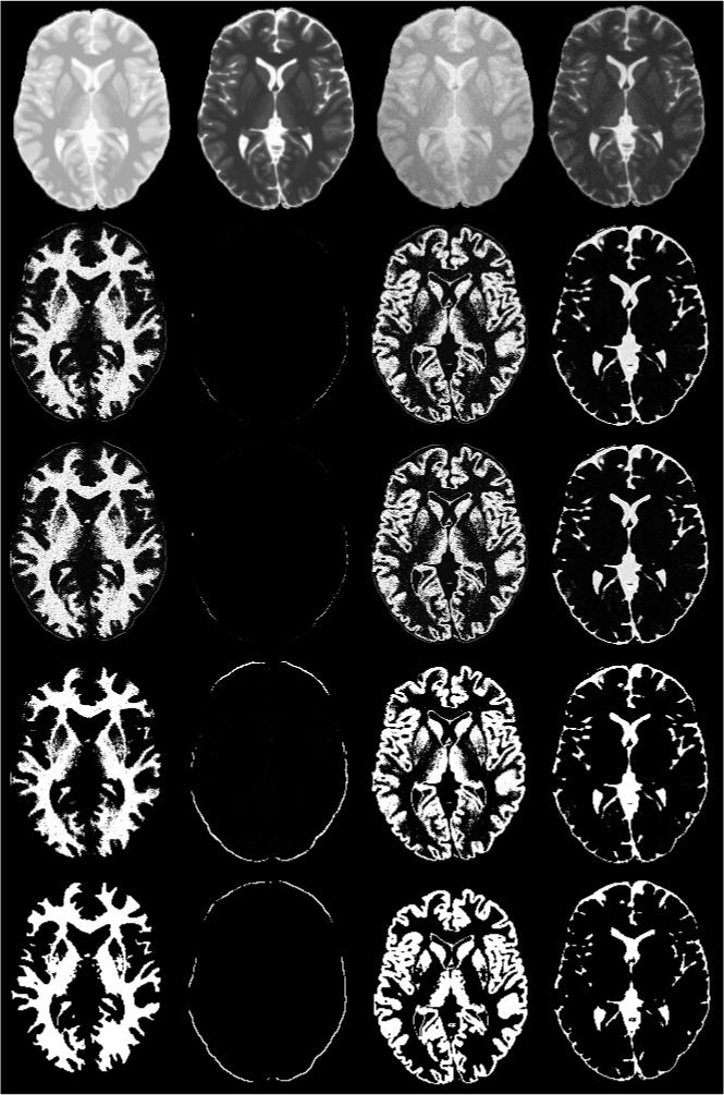
Classification of a Brainweb images into four tissue classes. The left two images in the first row are the original PD and T2 and the next two images are with 3% noise and 40% bias. The classification order in next four rows from left to right is WM, Dura, GM, and CSF. The second, third, and fourth rows show results with AFCM, G-K algorithm, and G-G algorithm, respectively. The last row shows the ground truth of Brainweb images.

Table 1.

Quantitative evaluation of AFCM, G-K and G-G methods for Brainweb images without applying neighbor contextual constraints (%), the results of FSL are included too.

	AFCM			G-K			G-G			FSL
	WM	GM	CSF	WM	GM	CSF	WM	GM	CSF	WM	GM	CSF
SI	89.7275	75.5651	73.3794	89.6643	88.7303	97.7046	91.5163	93.2882	97.3640	91.1051	92.2291	89.9979
POE	6.5546	10.0034	72.1330	5.83764	14.9534	4.4711	3.36327	11.3430	0.0878	14.9025	4.17254	1.79927
PUE	13.2976	33.1987	0.2452	13.9910	8.3321	0.2174	12.8033	2.66319	5.05324	3.86881	10.8503	16.7132
PCE	86.7024	66.8013	99.7548	86.0090	91.6679	99.7826	87.1967	97.3368	94.9468	96.1312	89.1497	83.2868

To evaluate the imhomogeneity correction, we calculated the image entropies before and after correction, and the results are summarized in Table 2. As can be seen from these results, all the three algorithms reduced the entropy, suggesting their effectiveness in correcting the bias field. These results also demonstrate the superior performance of the G-G and G-K algorithms relative to AFCM. The effect of membership contextual information on the similarity measures was investigated over a narrow range of the parameters α and β (0 to 0.1). Since the cost functions for the AFCM and G-K algorithms are different, one would expect the values of α and β to be different for these two algorithms. Based on this evaluation, the parameters that gave the best results were α = 0.1 and β = 0 for AFCM, α =0.01 and β =0 for G-K. As can be seen from this table, the contextual constraints considerably improved the segmentation performance. Fine tuning these parameters could further improve the results.

Table 2.

Calculated entropies of Brainweb images with AFCM, G-K and G-G methods. The entropy of the original images without inhomogeneity correction is shown in the last column.

Inhomogeneity Corrected	AFCM	G-K	G-G	Uncorrected
PD (1D)	7.1409	7.1053	7.1055	7.3414
T2 (1D)	7.5243	7.5198	7.5212	7.5526
PD-T2 (2D)	12.852	12.822	12.822	13.023

As an example, the calculated bias field profile in normal volunteer at two slice locations are shown in Fig. 2. These field profiles were generated using third order polynomial basis functions. This figure also shows the corresponding images before and after bias field correction. The substantial improvement in the image quality following the bias field correction can be visually appreciated on these images.

Figure 2.

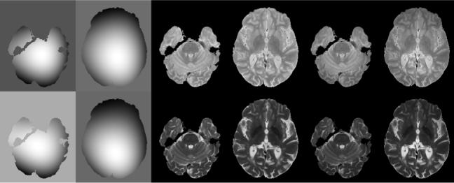
The imhomogeneity correction of FSE image obtained by applying G-G algorithm on two slices of images displayed in Fig.3 and Fig. 4. The first row is for PD, and the 2^nd row is for T2. The imhomogeneity are retrieved as columns 1 and 2, columns 3 and 4 are images before correction, and columns 5 and 6 are images after correction.

As indicated earlier, the images acquired on normal volunteers were classified into four classes namely GM, WM, CSF and GM+CSF. The use of four clusters in the FSE images (GM, WM, CSF, GM+CSF) can also be rationalized by the fact that the proximity of CSF and GM, particularly in the cortex, often results in significant partial volume averaging between these two tissues. Additional dimensions (represented by FLAIR images, for example) in the feature space may be required to increase the separability of more classes such as lesions ^{4, 17, 22}. As an example Fig. 3 shows the segmentation (membership) of one section of the brain in the cerebellar region. As can be seen from this figure, AFCM misclassified GM and WM (top row). However, both G-K and G-G correctly classified GM and WM (rows 2−4). Based on our own experience and that of a number of other investigators, the cerebellar and the posterior fossa regions are difficult to segment using FCM-based techniques ^{41, 44, 53}. It is known that on the FSE images the tissue intensities in the cerebellar regions are different from those of the superior parts of the brain ⁴⁴. This is especially evident in the scanning of clinical patients. These intensity differences can not be corrected by merely applying the inhomogeneity correction. Therefore, the segmentation of the cerebellum area is usually performed by adopting regional or localized methods ^{41, 44, 53}. With G-K/G-G algorithm, the segmentation is considerably improved.

Figure 3.

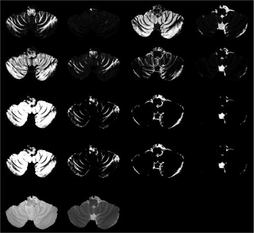
The membership of one axial cross-section of FSE images in cerebellum region, the classification is in the order of WM, GM, GM+CSF, and CSF, from left to right. The first row is the results of AFCM, the 2nd row is the results of G-K algorithm, and the 3rd row is the results of G-G algorithm with initials from AFCM, and the 4th row is the results of G-G algorithm with initials from G-K. The last row shows the original FSE images.

Fig. 4 shows the segmentation of a FSE image containing the thalamus/putamen structure. As can be seen from Fig. 3, the AFCM and G-K algorithms did not clearly discern the thalamus/putamen structure, while the G-G algorithm was able to segment these structures in a way that is consistent with the known anatomy. This pattern was consistently observed across all the images of the 20 volunteers that were included in these studies. It should be pointed out that, unlike in the real human images, the caudate/putamen structure in the Brainweb image was reasonably well segmented by the AFCM algorithm. This points out some of the limitations in using simulated images, such as Brainweb, for complete evaluation of segmentation algorithms.

Figure 4.

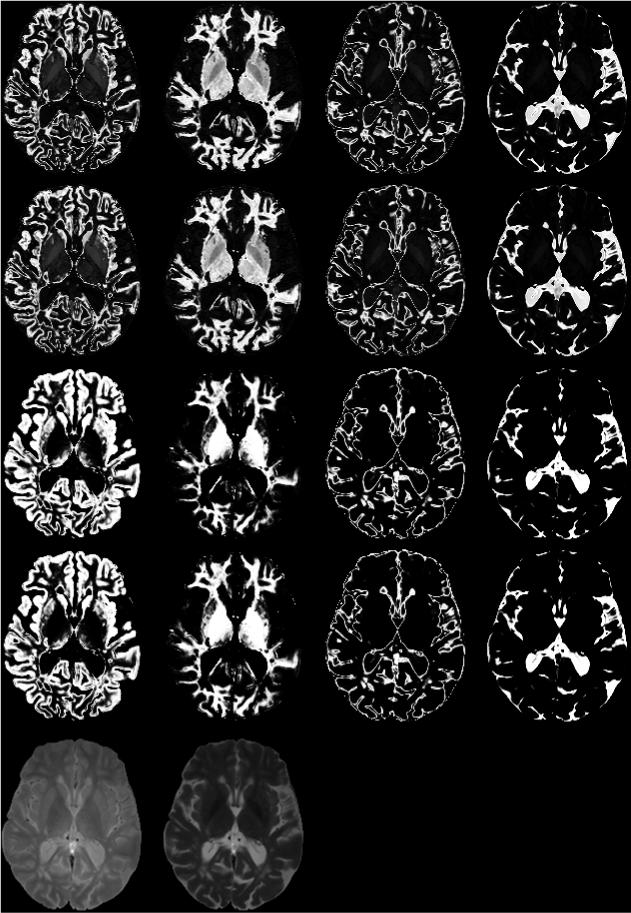
The membership of one axial cross-section of FSE images containing thalamus/putamen structure, the classification is in the same order of Figure 3. The first row is the results of AFCM, the 2nd row is the results of G-K algorithm, the 3rd row is the results of G-G algorithm with initials from G-K, and the 4th row is the results of G-G algorithm with initials from AFCM. The last row shows the original FSE images.

While we studied the segmentation of GM, WM, and CSF by including the volume and shape of clusters in the 2D feature space, additional dimensions in the feature space would be helpful in the segmentation of lesions. In addition, more complicated methods such as those described in ^{27, 11} would be helpful in increasing the computational efficiency. Further performance improvement could be obtained by considering the grand mean and cluster scatter matrices within and between clusters in the unsupervised clustering ^{45, 19, 8, 9, 12, 5, 6, 28, 29, 39, 52}.

Conclusions

An integrated approach for segmentation of multi-spectral MR images is described. This integrated approach incorporates an efficient bias field correction along with contextual constraints. This method takes into account the nonspherical occupancy and volume differences in the clusters in the feature space by replacing the Euclidian distance with cluster scatter measures to define the Mahalanobis distance, or fuzzifying the statistical measure of expectation-maximization. Qualitative and quantitative evaluation indicates satisfactory performance of this approach.

Table 3.

Quantitative evaluation of membership contextual constraints (%) (α = 0.1 and β =0 for AFCM, and α =0.01 and β =0 for G-K).

	AFCM			G-K
	WM	GM	CSF	WM	GM	CSF
SI	89.8555	80.2885	78.3481	91.2838	90.6280	98.8351
POE	6.7314	9.8808	54.2657	3.4493	14.9132	1.9871
PUE	12.9289	26.3047	0.6475	13.1386	4.7804	0.3616
PCE	87.0711	73.6953	99.3525	86.8614	95.2196	99.6384

Appendix I Extension of adaptive FCM to multi-channel segmentation

Denote

$$D_{ik}={\Vert {\mathbf{y}}_k-\mathbf{C}\Phi \left(p_k\right)+\mathbf{e}-{\mathbf{v}}_i\Vert }^2$$ (44)

and

$${{\rm Y}}_{ik}=\sum _{r\mid {\mathbf{y}}_r\in N_k}\left(\frac{\alpha }{N_R}{\Vert {\mathbf{y}}_r-\mathbf{C}\Phi \left(p_r\right)+\mathbf{e}-{\mathbf{v}}_i\Vert }^2+\frac{\beta }{N_R}\sum _{m\ne k}{u}_{rm}^p\right)$$ (45)

The Lagrange multiplier is adopted to include the constraints into the optimization and the augmented objective function becomes

$$F=\sum _{i=1}^c\sum _{k=1}^N(u_{ik}^p{D}_{ik}+u_{ik}^p{{\rm Y}}_{ik})+\lambda \left(1-\sum _{i=1}^c{u}_{ik}\right)$$ (46)

Taking the derivative of F with u_ik, for p>1, we have

$${\left[\frac{\partial F}{\partial u_{ik}}=p{u}_{ik}^{p-1}{D}_{ik}+p{u}_{ik}^{p-1}{{\rm Y}}_{ik}-\lambda \right]}_{u_{ik}=u_{ik}^{\ast }}=0$$ (47)

and

$$u_{ik}={(\lambda ∕\left(p(D_{ik}+{{\rm Y}}_{ik})\right))}^{1∕(p-1)}$$ (48)

by applying ${\sum }_{j=1}^c{u}_{jk}=1$, we have

$$\lambda =p/{\left(\sum _{j=1}^c{(1∕(D_{jk}+{{\rm Y}}_{jk}))}^{1∕(p-1)}\right)}^{(p-1)}$$ (49)

and

$$u_{ik}=1/\sum _{j=1}^c{\left(\frac{D_{ik}+{{\rm Y}}_{ik}}{D_{jk}+{{\rm Y}}_{jk}}\right)}^{1∕(p-1)}$$ (50)

The concrete norm is required to derive the updated cluster prototype. Generally the norm is given by

$${\Vert \mathbf{x}\Vert }^2={\mathbf{x}}^{\mathbf{T}}\mathbf{Lx}$$ (51)

where L is a positive definite matrix, by using (16), for Euclidean norm, we have L=I, the identity matrix. Taking the derivative of F with respect to v_i, we have

$${\left[\sum _{k=1}^N{u}_{ik}^p({\mathbf{y}}_k-\mathbf{C}\Phi \left(p_k\right)+\mathbf{e}-{\mathbf{v}}_i)+\sum _{k=1}^N{u}_{ik}^p\frac{\alpha }{N_R}\sum _{r\mid {\mathbf{x}}_r\in N_k}({\mathbf{y}}_r-\mathbf{C}\Phi \left(p_r\right)+\mathbf{e}-{\mathbf{v}}_i)\right]}_{{\mathbf{v}}_i={\mathbf{v}}_i^{\ast }}=0$$ (52)

and

$${\mathbf{v}}_i=\frac{\sum _{k=1}^N{u}_{ik}^p\left(({\mathbf{y}}_k-\mathbf{C}\Phi \left(p_k\right)+\mathbf{e})\frac{\alpha }{N_R}\sum _{r\mid {\mathbf{x}}_r\in N_k}({\mathbf{y}}_r-\mathbf{C}\Phi \left(p_r\right)+\mathbf{e})\right)}{(1+\alpha )\sum _{k=1}^N{u}_{ik}^p}$$ (53)

Similarly, the bias field can be estimated by taking the derivative of F with b_k, that is

$$\begin{array}{cc}\hfill & \frac{\partial }{\partial \mathbf{C}}[\sum _{i=1}^c\sum _{k=1}^N(u_{ik}^p{({\mathbf{y}}_k-\mathbf{C}\Phi \left(p_k\right)+\mathbf{e}-{\mathbf{v}}_i)}^T({\mathbf{y}}_k-\mathbf{C}\Phi \left(p_k\right)+\mathbf{e}-{\mathbf{v}}_i)\hfill \\ \hfill & {+\sum _{r\mid {\mathbf{y}}_r\in N_k}\left(\frac{\alpha }{N_R}{({\mathbf{y}}_r-\mathbf{C}\Phi \left(p_r\right)+\mathbf{e}-{\mathbf{v}}_i)}^T({\mathbf{y}}_r-\mathbf{C}\Phi \left(p_r\right)+\mathbf{e}-{\mathbf{v}}_i)\right))]}_{\mathbf{C}={\mathbf{C}}^{\ast }}=0\hfill \end{array}$$ (54)

and using the formula of (19), Eqn. (54) can be written as

$$\begin{array}{cc}\hfill & \frac{\partial }{\partial \mathbf{C}}[\sum _{i=1}^c\sum _{k=1}^N(u_{ik}^p{({\mathbf{y}}_k-\mathbf{C}\Phi \left(p_k\right)+\mathbf{e}-{\mathbf{v}}_i)}^T({\mathbf{y}}_k-\mathbf{C}\Phi \left(p_k\right)+\mathbf{e}-{\mathbf{v}}_i)+\hfill \\ \hfill & {\sum _{r\mid {\mathbf{y}}_r\in N_k}\left(\frac{\alpha }{N_R}{({\mathbf{y}}_r-\mathbf{C}\Phi \left(p_r\right)+\mathbf{e}-{\mathbf{v}}_i)}^T({\mathbf{y}}_r-\mathbf{C}\Phi \left(p_r\right)+\mathbf{e}-{\mathbf{v}}_i)\right))]}_{\mathbf{C}={\mathbf{C}}^{\ast }}=0\hfill \end{array}$$ (55)

then we get

$$\begin{array}{cc}\hfill & \mathbf{C}\sum _{i=1}^c\sum _{k=1}^N{u}_{ik}^p(\left[\Phi \left(p_k\right)\right]{\left[\Phi \left(p_k\right)\right]}^T+\sum _{r\mid {\mathbf{y}}_r\in N_k}\frac{\alpha }{N_R}\left[\Phi \left(p_r\right)\right]{\left[\Phi \left(p_r\right)\right]}^T)\hfill \\ \hfill & =\sum _{i=1}^c\sum _{k=1}^N{u}_{ik}^p(({\mathbf{y}}_k+\mathbf{e}-{\mathbf{v}}_i){\left[\Phi \left(p_k\right)\right]}^T+\sum _{r\mid {\mathbf{y}}_r\in N_k}\frac{\alpha }{N_R}({\mathbf{y}}_r+\mathbf{e}-{\mathbf{v}}_i)\left[\Phi {\left(p_r\right)}^T\right])\hfill \end{array}$$ (56)

Solving Eqn. (56) leads to the smooth approximation of the bias field as

$$\begin{array}{cc}\hfill {\mathbf{b}}_{k\left(smooth\right)}& ={[\sum _i{c}_{1i}{\varphi }_i\left(p_k\right),\sum _i{c}_{2i}{\varphi }_i\left(p_k\right),\dots ,\sum _i{c}_{ni}{\varphi }_i\left(p_k\right)]}^T\hfill \\ \hfill & =\mathbf{C}\Phi \left(p_k\right)\hfill \end{array}$$ (57)

References

- 1.Ahmed MN, Yamany SM, Mohamed N, Farag AA, Moriarty T. A modified fuzzy c-means algorithm for bias field estimation and segmentation of MRI data. IEEE Trans Med Imag. 2002;21:193–199. doi: 10.1109/42.996338. [DOI] [PubMed] [Google Scholar]
- 2.Alirezaie J, Jernigan ME. MR image segmentation and analysis based on neural network. In: Yan H, editor. Signal Processing for Magnetic Resonance Imaging and Spectroscopy. Marecel Dekker; New York: 2002. [Google Scholar]
- 3.Anbeek P, Vincken KL, van Osch MJP, Bisschops RHC, Grond J. Probabilistic segmentation of white matter lesions in MR imaging. NeuroImage. 2004;21:1037–1044. doi: 10.1016/j.neuroimage.2003.10.012. [DOI] [PubMed] [Google Scholar]
- 4.Bedell BJ, Narayana PA, Wolinsky JS. A dual approach for minimizing false lesion classifications on magnetic resonance images. Magn Reson Med. 1997;37:94–102. doi: 10.1002/mrm.1910370114. [DOI] [PubMed] [Google Scholar]
- 5.Bensaid AM, Hall LO, Bezdek JC, Clarke LP. Partially supervised clustering for image segmentation. Pattern Recognition. 1996a;29:859–871. [Google Scholar]
- 6.Bensaid AM, Hall LO, Bezedek JC, Clarke LP, Silbiger ML, Arrington JA, Murtagh RF. Validity-guided reclustering with applications to image segmentation. IEEE Trans Fuzzy Syst. 1996b;4:112–123. [Google Scholar]
- 7.Bermel RA, Bakshi R. The measurement and clinical relevance of brain atrophy in multiple sclerosis. Lancet Neurol. 2006;5:158–70. doi: 10.1016/S1474-4422(06)70349-0. [DOI] [PubMed] [Google Scholar]
- 8.Bezdek JC. PhD Thesis. Cornell University; 1973. Fuzzy Mathematics in Pattern Classification. [Google Scholar]
- 9.Bezdek JC. A convergence theorem for the fuzzy ISODATA clustering algorithms. IEEE Trans Pattern Anal Machine Intell. 1980;2:1–8. doi: 10.1109/tpami.1980.4766964. [DOI] [PubMed] [Google Scholar]
- 10.Bezdek JC, Ehrlich R, Full. W. FCM: Fuzzy c-Means Algorithm. Computers and Geoscience. 1984;10:191–203. [Google Scholar]
- 11.Borgelt C, Kruse R. Shape and size regularization in expectation maximization and fuzzy clustering.. Proc 8th Euro Conf Principles Practice Knowledge Discovery Databases (PKDD).2004. pp. 52–62. [Google Scholar]
- 12.Clark MC, Hall LO, Goldgof DB, Clarke LO, Velthuizen RP, Silbiger MS. MRI segmentation using fuzzy clustering techniques. IEEE Eng Med Bio. 1994;13:730–742. [Google Scholar]
- 13.Cocosco CA, Kollokian V, Kwan RK-S, Evans AC. Brainweb: online interface to a 3D MRI simulated brain database. NeuroImage. 1997;5:S425–427. http://www.bic.mni.mcgill.ca/brainweb/
- 14.Datta S, Sajja BR, He R, Wolinsky JS, Gupta RK, Narayana PA. Segmentation and quantification of black holes in multiple sclerosis. Neuroimage. 2006;29:467–474. doi: 10.1016/j.neuroimage.2005.07.042. [DOI] [PMC free article] [PubMed] [Google Scholar]
- 15.Dawant BM, Zijdenbos AP, Margolin RA. Correction of intensity variations in MR images for computer-aided tssue classification. IEEE Trans Med Imag. 1993;12:770–781. doi: 10.1109/42.251128. [DOI] [PubMed] [Google Scholar]
- 16.Dempster AP, Laird NM, Rubin DB. Maximum likelihood from incomplete data via the EM algorithm. J Roy Statist Soc B. 1977;39:1–38. [Google Scholar]
- 17.Ding Z, Preiningerova J, Cannistraci CJ, Vollmer TL, Gore JC, Anderson AW. Quantification of multiple sclerosis lesion load and brain tissue volumetry using multiparameter MRI: methodology and reproducibility. Magn Reson Imag. 2005;23:445–452. doi: 10.1016/j.mri.2004.12.005. [DOI] [PubMed] [Google Scholar]
- 18.Gath I, Geva AB. Unsupervised optimal fuzzy clustering. IEEE Trans Pattern Anal Machine Intell. 1989;11:773–781. [Google Scholar]
- 19.Gunn JC. A fuzzy relative of the ISODATA process and its use in detecting compact, well separated clusters. J Cybern. 1974;3:95–104. [Google Scholar]
- 20.Gustafson DE, Kessel WC. Fuzzy clustering with a fuzzy covariance matrix.. Proc IEEE Conf Decision Contr.1979. pp. 761–766. [Google Scholar]
- 21.He R, Datta S, Sajja BR, Mehta M, Narayana PA. Adaptive FCM with contextual constraints for segmentation of multi-spectral MRI. Proc of IEEE Engg Med Bio Soc (EMBS) 2004:1660–1663. doi: 10.1109/IEMBS.2004.1403501. [DOI] [PubMed] [Google Scholar]
- 22.He R, Sajja BR, Narayana PA. Implementation of high dimensional feature map for segmentation of MR images. Annals Biomed Engg. 2005;33:1439–1448. doi: 10.1007/s10439-005-5888-3. [DOI] [PMC free article] [PubMed] [Google Scholar]
- 23.Höppner F, Klawonn F. A contribution to convergence theory of fuzzy c-means and derivatives. IEEE Trans Fuzzy Syst. 2003;11:682–694. [Google Scholar]
- 24.Höppner F, Klawonn F, Kruse R, Runkler TA. Fuzzy Cluster Analysis. Wiley; Chichester: 1999. [Google Scholar]
- 25.Inglese M, Grossman RI, Filippi M. Magnetic resonance imaging monitoring of multiple sclerosis lesion evolution. J Neuroimaging. 2005;15(4 Suppl):22S–29S. doi: 10.1177/1051228405282243. [DOI] [PubMed] [Google Scholar]
- 26.Jiang L, Yang W. A modified fuzzy c-means algorithm for segmentation of magnetic resonance images.. Proceedings of the Seventh International Conference on Digital Image Computing: Techniques and Applications.; CSIRO Publishing, Sydney. 2003. pp. 225–232. [Google Scholar]
- 27.Keller A, Klawonn F. Adaptation of cluster sizes in objective function based fuzzy clustering. In: Leondes CT, editor. Database and Learning Systems IV. CRC Press; Boca Raton: 2003. pp. 181–199. [Google Scholar]
- 28.Krishnapuram R, Kim J. A note on the Gustafson–Kessel and adaptive fuzzy clustering algorithms. IEEE Trans Fuzzy Syst. 1999;7:453–461. [Google Scholar]
- 29.Krishnapuram R, Kim J. Clustering algorithms based on volume criteria. IEEE Trans Fuzzy Syst. 2000;8:228–236. [Google Scholar]
- 30.Li DK, Li MJ, Traboulsee A, Zhao G, Riddehough A, Paty D. The use of MRI as an outcome measure in clinical trials. Adv Neurol. 2006;98:203–26. [PubMed] [Google Scholar]
- 31.Liew AW-C, Yan H. An adaptive spatial fuzzy clustering algorithm for 3-D MR image segmentation. IEEE Trans Med Imag. 2003;22:1063–1075. doi: 10.1109/TMI.2003.816956. [DOI] [PubMed] [Google Scholar]
- 32.Liew AW-C, Yan H. Current methods in automatic tissue segmentation of 3D magnetic resonance brain images. Curr Med Iamging Rev. 2006;2:91–103. [Google Scholar]
- 33.Lycklama a Nijeholt GJ. Reduction of brain volume in MS. MRI and pathology findings. J Neurol Sci. 2005;233(1−2):199–202. doi: 10.1016/j.jns.2005.03.016. [DOI] [PubMed] [Google Scholar]
- 34.Matthews B, Siemers ER, Mozley PD. Imaging-based measures of disease progression in clinical trials of disease-modifying drugs for Alzheimer disease. Am J Geriatr Psychiatry. 2003;11(2):146–59. [PubMed] [Google Scholar]
- 35.McLachlan GJ, Basford KE. Mixture Models: Inference and Applications to Clustering. Marecel Dekker; New York: 1988. [Google Scholar]
- 36.McLachlan GJ, Krishnan T. The EM Algorithm and Extensions. John Wiley and Sons; New York: 1997. [Google Scholar]
- 37.Pham DL. Spatial models for fuzzy clustering. Computer Vision and Image Understanding. 2001;84:285–297. [Google Scholar]
- 38.Pham DL, Prince JL. Adaptive fuzzy segmentation of magnetic resonance images. IEEE Trans Med Imag. 1999;18:737–752. doi: 10.1109/42.802752. [DOI] [PubMed] [Google Scholar]
- 39.Rouseeuw PJ, Kaufman L, Trauwaert E. Fuzzy clustering using scatter matrices. Comput Stat Data Anal. 1996;23:135–151. [Google Scholar]
- 40.Sahoo P, Soltani S, Wong A, Chen Y. A survey of thresholding techniques. Comp Vision Graph Imag Proc. 1988;41:233–260. [Google Scholar]
- 41.Sajja BR, Datta S, He R, Mehta M, Gupta RK, Wolinsky JS, Narayana PA. Unified approach for multiple sclerosis lesion segmentation on brain MRI. Annals Biomed Engg. 2006;34:142–151. doi: 10.1007/s10439-005-9009-0. [DOI] [PMC free article] [PubMed] [Google Scholar]
- 42.Sittigorn J, Rangsanseri Y, Thitimajshima P. Incorporating spatial information into fuzzy clustering of multi-spectral images.. Asian Conference on Remote Sensing, Poster 135..2002. [Google Scholar]
- 43.Sled JG, Zijdenbos AP, Evans AC. A nonparametric method for automatic correction of intensity non-uniformity in MRI data. IEEE Trans Med Imag. 1998;17:87–97. doi: 10.1109/42.668698. [DOI] [PubMed] [Google Scholar]
- 44.Suckling J, Sigmundsson T, Greenwood K, bullmore ET. A modified fuzzy clustering algorithm for operator independent brain tissue classification of dual echo MR images. Magn Reson Imag. 1999;17:1065–1076. doi: 10.1016/s0730-725x(99)00055-7. [DOI] [PubMed] [Google Scholar]
- 45.Sutton MA, Bezdek JC, Cahoon TC. Image segmentation by fuzzy clustering: methods and issues. In: Bankman IN, editor. Handbook of Medical Imaging: Processing and Analysis. Academic Press; San Diego: 2000. pp. 87–106. [Google Scholar]
- 46.Taxt T, Lundervold A. Multi-spectral analysis of the brain using magnetic resonance imaging. IEEE Trans Med Imag. 1994;13:470–481. doi: 10.1109/42.310878. [DOI] [PubMed] [Google Scholar]
- 47.Tincher M, Meyer CR, Gupta R, Williams DM. Polynomial modeling and reduction of RF body coil spatial inhomogeneity in MRI. IEEE Trans Med Imag. 1993;12:361–365. doi: 10.1109/42.232267. [DOI] [PubMed] [Google Scholar]
- 48.Van Leemput K, Meas F, Vandermeulen D, Suetens P. Automated model-based bias field correction of MR images of the brain. IEEE Trans Med Imag. 1999;18:885–896. doi: 10.1109/42.811268. [DOI] [PubMed] [Google Scholar]
- 49. WWW.fil.ion.ucl.ac.uk/spm/software/spm5/
- 50. WWW.fmrib.ox.ac.uk/fsl/
- 51.Xue J-H, Pizurica A, Philips W, Kerre E, van De Walle R, Lemachieu I. An integrated method of adaptive enhancement for unsupervised segmentation of MRI brain images. Pattern Recognition Letters. 2003;24:2549–2560. [Google Scholar]
- 52.Yang MS. PhD Thesis. Chung Yuan Christian University; 2004. Fuzzy Clustering Algorithms Based on Scatter Matrices. [Google Scholar]
- 53.Zhu C, Jiang T. Multicontext fuzzy clustering for separation of brain tissues in magnetic resonance images. NeuroImage. 2003;18:685–696. doi: 10.1016/s1053-8119(03)00006-5. [DOI] [PubMed] [Google Scholar]