Contour Statistics in Natural Images

Abstract

Correctly interpreting a natural image requires dealing properly with the effects of occlusion, and hence contour grouping across occlusions is a major component of many natural visual tasks. To better understand the mechanisms of contour grouping across occlusions we (a) measured the pair-wise statistics of edge elements from contours in natural images, as a function of edge-element geometry and contrast polarity, (b) derived the ideal Bayesian observer for a contour occlusion task where the stimuli were extracted directly from natural images, and then (c) measured human performance in the same contour occlusion task. In addition to discovering new statistical properties of natural contours, we found that naïve human observers closely parallel ideal performance in our contour occlusion task. In fact, there was no region of the four-dimensional stimulus space (3 geometry dimensions and 1 contrast dimension) where humans did not closely parallel the performance of the ideal observer (i.e., efficiency was approximately constant over the entire space). These results reject many other contour grouping hypotheses and strongly suggest that the neural mechanisms of contour grouping are tightly related to the statistical properties of contours in natural images.

Introduction

It is common in natural scenes for an object to be partially occluded by one or more other objects (Fig. 1). Such occlusions can provide useful depth and segmentation (figure-ground) information; for example, if the bounding contour of an object can be identified, then other contours intersecting that bounding contour are likely to be occluded, and hence likely to be at a greater distance and to derive from a different physical source than the bounding contour (e.g., a different object). However, the existence of occlusions can also greatly increase the difficulty of correctly interpreting natural images; for example, an occluding object necessarily obscures image features from the occluded objects, making identification of the occluded objects difficult.

Figure 1.

Examples of occlusion in natural scenes.

The human visual system contains powerful contour grouping mechanisms that are thought to play an important role in helping the visual system both exploit occlusions and overcome the loss of features produced by occlusions (e.g., Rock 1975; Barrow & Tenenbaum 1986; Kellman 2003). For example, contour grouping mechanisms allow us to decide (correctly) that the two contours passing under the red leaf in Fig. 1 arise from the same physical source (surface boundary). These contour grouping mechanisms undoubtedly evolved and/or develop in response to the properties of natural environments, and thus there have been recent efforts to directly measure the statistical properties of contours in natural images, with the aim of gaining a deeper understanding of the image information available to support contour grouping and of developing more refined models of contour grouping (Geisler et al. 2001; Elder & Goldberg 2002; Martin et al. 2004).

One approach has been to extract contour elements from natural images using an automatic edge detection algorithm and then examine the pair-wise statistics of the extracted contour elements. Using this approach Sigman et al. (2001) and Geisler et al. (2001) examined the statistics of the geometrical relationship between contour elements and found that there is a local maximum in the pair-wise probability distribution for edge elements that are approximately co-circular (i.e., are approximately tangent to a common circle, but see later). Geisler et al. (2001) also showed that there is a larger local maximum for edge elements that are approximately parallel (i.e., are approximately tangent to parallel lines). These two properties undoubtedly reflect the fact that natural contours are relatively smooth (e.g., the bounding contours of a branch or leaf in Fig. 1), and that natural images contain many parallel contours (e.g., the two sides of a branch or leaf in Fig. 1). Such measurements of pair-wise statistics can identify important statistical structure that is relevant for grouping; however, the measurements are obtained completely within the domain of images.

Potentially more relevant statistical relationships can be obtained by measuring across-domain statistics, which involves measurements both within images as well as within the corresponding environments in order to obtain ground truth information. Measurements of ground truth are essential for determining how a rational observer should use image information when interacting with, or drawing inferences about, the environment. (For more discussion of the distinction between within-domain and across-domain statistics see Geisler 2008.) Direct measurement of ground truth information can be difficult, and thus a common shortcut is to exploit hand segmentation by human observers (Brunswik & Kamia 1953; Geisler, et al. 2001; Elder & Goldberg 2002; Martin et al. 2004). The premise of this approach is that under some circumstances human observers can make veridical assignments of image pixels to physical sources in the environment. To the extent that this assumption holds (see later), the assignment data can provide useful ground truth information.

The present study uses the hand segmentation database for natural images reported in Geisler et al. (2001). In that study we applied an automatic algorithm to detect local contour elements (at a small spatial scale) in a diverse collection of natural images, and then had observers assign the elements to physical sources (surface/material boundary contours, shadow/shading contours, or surface marking contours). The earlier study only considered the statistics of the geometrical relationship between contour elements. In the current study, we extend the statistical analysis to include the contrast relationship between contour elements (specifically the contrast polarity). We then describe a contour grouping experiment where subjects are required to decide whether a pair of contour elements at the boundary of an occluder belongs to the same or different physical contours. We then compare human performance in this task with that of a parameter-free ideal observer that directly uses the measured natural scene statistics to perform the contour occlusion task. A preliminary report of the study described here appeared in an SPIE conference proceedings (Geisler et al., 2008).

Methods

Natural Contour Statistics

Much of the procedure for measuring contour statistics is described elsewhere (Geisler et al. 2001). Briefly, we analyzed a set of natural images (480 × 480 pixels) that were picked to be as diverse as possible, without containing human-made objects or structures. The images included close-up and distant views of different environments (i.e., forests, mountains, deserts, plains, seashore) and image constituents (e.g., water, sky, snow, plants, trees and rocks). Small regions cut from three of the images are shown at the top of Fig. 2 (thumb nails of all the full images can be found in Geisler et al. 2001; also see Fig. 3a).

Figure 2.

Contour locations and contour groups for small example patches from three different natural images. The contour locations and contrast polarities were detected by an automatic algorithm. The contour groups were obtained by hand segmentation. The direction of the arrows in the bottom images indicates the contrast polarity of the contour; the different colors represent different groups (note that because colors are randomly selected from a color palette, different groups may have a similar color).

Figure 3.

Definition of parameters describing the geometrical and contrast relationship between a pair of contour elements.

Edges were extracted from each image using an automatic algorithm containing the following steps: (a) convert the image to gray scale, (b) filter the gray scale image with a non-oriented log Gabor filter (in the Fourier domain) having a spatial-frequency bandwidth of 1.5 octaves and a peak spatial frequency of 0.1 c/pixel (the frequency was picked to provide a dense sampling of contours), (c) identify the locations of zero crossings in the filtered image, (d) at each zero crossing point in the (unfiltered) gray scale image apply a bank of odd and even log Gabor filters with a spatial-frequency bandwidth of 1.5 octaves, a peak spatial frequency of 0.1 c/pixel, and an orientation bandwidth of 40 deg, (e) normalize the filter responses by dividing by the sum of the responses across all orientations, (f) combine the odd and even responses to obtain an energy response, (g) find the peak of the energy response across orientation to determine the local contour orientation, (h) eliminate edge elements with peak normalized energy responses that do not exceed a low threshold, (i) interpolate the even and odd responses to better localize the edge position, (j) reapply an odd log Gabor filter at the estimated edge-element orientation and position in the gray scale image to determine the contrast polarity (the sign of the contrast) of the edge element. The last two steps were not applied in the original study (Geisler et al. 2001). The above edge extraction procedure was applied to synthetic test images with known contour positions, orientations and contrast polarities, and was found to be accurate for the test images.

We note that the extraction of contrast polarity information is new to the current study. We chose not to examine contrast magnitude because the images were neither luminance nor color calibrated, and thus for these images we can only be confident about measurements of edge geometry and contrast polarity.

The colored pixels in the middle panels of Fig. 2 are examples of the locations of extracted edge elements. The arrows in the bottom panels of Fig. 2 show a small subset of the extracted edge elements. The center point of an arrow indicates the position of the edge element (corresponding to a pixel in the middle panels) and the orientation of the arrow indicates the orientation of the edge element. Reversals in arrow direction indicate flips in contrast polarity.

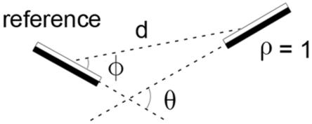
We measured both the within-domain and the across-domain statistics of edge geometry and contrast polarity. For both we measured pair-wise statistics. Specifically, for each pairing of extracted edge elements we considered one of them as the reference and described the geometrical and contrast relationship of the other element relative to the reference element (every edge element served as a reference element). Thus, we average over the absolute orientation of the reference element. The relationship between the elements is described by four parameters (Fig. 3): the distance between the centers of the edge elements (d), the direction of the second element from the reference element (-90°≤ϕ≤90°), the orientation difference between the edge elements (-90°≤θ≤90°), and difference between the edge elements in contrast polarity (ρ=1, same polarity; ρ= 0, different polarity). Thus, the pair-wise statistics can be described by a four dimensional probability density function, p(d,ϕ,θ,ρ). This function was estimated by binning the edge element pairs along the four dimensions (6 distances x 36 directions x 36 orientation-differences x 2 contrast polarities for a total of 15552 bins). This four-dimensional probability distribution summarizes the within-domain statistics of edge element geometry and contrast polarity. We briefly describe these statistics in the results section, but the statistics of primary interest here are the across-domain statistics, which were obtained using the hand segmentation results.

For the across-domain statistics we first had two observers segment the extracted edge elements into groups that belong to the same physical contour. The observers viewed the images with each extracted edge element labeled by a single colored pixel (e.g., middle panels in Fig. 2). They then selected those pixels that belong to the same contour (e.g., the yellow pixels in the middle panels). To aid them in the segmentation they were allowed to zoom in and out, toggle to the full color image (upper panels), and toggle the colored pixels on and off. The fundamental premise here is that most of the segmentations correspond to the physical ground truth (i.e., the grouped pixels do indeed arise from a common physical source—a surface/material boundary, a shadow/shading boundary, or surface marking boundary). The observers noted that some ambiguous cases arose, but that they were highly confident about most of the pixels assignments, which was supported by the high inter-observer agreement (Geisler et al. 2001; also see discussion). Given the segmentation data, it is then possible to estimate (by binning the edge element pairs) the across-domain probability distribution p(c,d,ϕ,θ,ρ), where c takes on two possible values: c =1 if the edge elements belong to the same contour and c = 0 if they belong to different contours. The images and segmented contours can be found at the following web site: http://www.cps.utexas.edu/kodakdb/.

Contour Occlusion Task

In the contour occlusion task, we measured subjects’ ability to identity whether a pair of edge elements passing under an occluder belonged to the same or different physical contours. On half the trials the edge elements belonged to the same contour and on half to different contours.

On each trial, a pair of edge elements was extracted directly from our database of natural images via the following procedure. First an image was randomly selected and then a single edge element was randomly selected from that image (e.g., one of the two green highlighted edge elements in Fig. 4a). Second, we considered the set of all edge elements at a given distance from the selected edge element, where the distance equaled the occluder diameter for that trial. On “different” trials we randomly selected an edge element from those that belonged to a physical contour different from the contour containing the initially selected element. On “same” trials we randomly selected from those elements (usually just one or two elements) that belonged to the same physical contour as the initial selected element (e.g., in Fig. 4a, the second green highlighted element belongs to the same physical contour). Same and different trials occurred randomly with equal probability and subjects were informed that the probabilities were equal. Forcing the prior probabilities to be equal is unnatural, but greatly reduces the number of trials required to obtain useful data. As will be seen below, subjects had no trouble dealing with equal prior probabilities.

Figure 4.

Contour occlusion task stimuli. The largest occluder diameter was 90 pixels (shown here), corresponding 3 deg of visual angle.

Once the edge elements were selected, they were displayed to the subject as shown in Fig. 4b. Specifically, the 480 × 480 pixel image subtended 16 deg in visual angle with a gray background luminance of 55 cd/m² and a gray, circular occluder of 60 cd/m². (The video mode was set to 1280 × 960 and the image upsampled to allow better anti-aliasing of the occluder boundary.) As in Fig. 4b, the 3.0 c/deg edge elements were always located on opposite ends of a line through the center of the occluder. The size of the edge elements in the display was the same as the size of the oriented filter kernels used to extract the edge elements when we measured the pair-wise statistics. The center pixel of the edge element sat on the occluder boundary. The contrast of the edge elements was set so that their locations and orientations were clearly visible (Michelson contrast = 0.6). On each trial, the display remained up until the subject responded, and the subject was free to make eye movements.

Performance was measured, in counterbalanced blocks, for occluder diameters of 20, 40, and 90 pixels (0.67 deg, 1.33 deg and 3 deg). (We note that it was not possible to measure performance for occluder diameters greater that 90 pixels because there are too few contours of sufficient length in the database.) In addition, we measured performance with and without the contrast polarity information; in the blocks where the polarity information was absent we replaced the odd symmetric edge elements with even symmetric elements.

Finally, we also manipulated feedback. For the first 600 trials of the experiment no feedback was provided; for the second 600 trials feedback was provided on each trial (a tone indicated whether the response was correct or incorrect); for the third block of 600 trials no feedback was provided. We chose to manipulate feedback because of concern that our occlusion displays were so simplified (unnatural) that subjects may not be able to use the edge geometry and contrast information in the way that they would normally use that information in natural images. We reasoned that if the subjects show no improvement with feedback then it strongly suggests that they are able to apply their normal contour processing mechanisms to our simplified displays.

Seven subjects participated in the study. Two were familiar with the aims of the study and five were naïve. On the first day (prior to the main experiment), each subject completed 10 trials designed to help them understand the task and display. Specifically, after each stimulus presentation and response (which was the same as in the main experiment), the subjects were shown a display like the one in Fig. 4a, which illustrated exactly how the simplified display was obtained from the original image. For the remainder of the study, the subjects only saw displays like the one in Fig. 4b. The study extended over a period of 3 to 6 days, depending on the subject.

Ideal Observer for Contour Occlusion Task

The only information available to perform the contour occlusion task is the geometrical relationship between the pair of edge elements, and in some conditions the geometrical and contrast-polarity relationship between the elements. Thus, using the measured contour statistics we can derive the performance of a rational (ideal) observer that has perfect knowledge of the natural scene statistics of edge element geometry and contrast polarity. An ideal observer that wishes to maximize accuracy will compare the posterior probability that the observed contour elements belong to the same physical contour with the posterior probability that they belong to different physical contours and then respond “same” if the former posterior probability is the larger:

$$\text{if}p(c=1\mid d,\varphi ,\theta ,\rho )>p(c=0\mid d,\varphi ,\theta ,\rho )\text{then respond}‘‘\text{same contour}"$$ (1)

In the Appendix, we show that this decision rule is identical to this one: ¹

$$\text{if}\frac{p(\varphi ,\theta ,\rho \mid d,c=1)}{p(\varphi ,\theta ,\rho \mid d,c=0)}>\frac{p(c=0\mid d)}{p(c=1\mid d)}\text{then respond}‘‘\text{same contour}"$$ (2)

The term on the left is a distance-dependent likelihood ratio: the probability of the observed direction, orientation and polarity relationship between the edge elements given the observed distance and that the elements belong to the same contour, divided by the probability of the same observed relationship between the elements given the observed distance and that they belong to different contours. We represent this likelihood ratio by l(ϕ,θ,ρ|d). The term on the right is the ratio of the prior probabilities that two edge elements separated by distance d belong to different versus the same contour. We represent this distance-dependent decision criterion by β (d). In the present contour occlusion task we forced the prior probability of the edge elements belonging to the same contour to be 0.5, and hence we forced the ideal criterion to be 1.0 (β(d)=1.0). The subjects were told that the prior probabilities were 0.5 before the start of the experiment. We applied equation (2) to each individual trial for each subject, which allowed us to compare human and ideal observer responses on a trial-by-trial basis.

Results

This section begins with a description of the pair-wise statistics of contour elements within natural images (the within domain statistics), followed by a description of the pair-wise statistics of contour elements referenced to the ground truth of whether the elements arise from the same or different physical sources (the across domain statistics). Finally we describe of the results of contour occlusion experiment and compare them with the predictions of an ideal observer that has full knowledge of the measured across-domain statistics.

Natural Contour Statistics: Within Domain

The within-domain statistics are shown in Fig. 5a, which plots the measured four-dimensional probability distribution, p(d,ϕ,θ,ρ), normalized to a peak of 1.0 for each distance bin. The reference element is not shown, but would be a horizontal element in the center of the diagram. Each of the line segments in the plot represents one of the 15, 552 bins covering the four-dimensional space (note that the line segments are so dense that they blend into solid regions.) In this figure, distance (d) from the reference is represented by the six rings, which correspond to the six distance bins. Direction (ϕ) is represented by the angular direction along a ring (range = ±90°; we can restrict this range to ±90° because a plot with a range of ±180°, for a given contrast polarity, is symmetric about the origin). Orientation difference (θ) is represented by the orientation of the line segment (range = ±90°) drawn at a given distance and direction. Contrast polarity (ρ) is represented by the two halves of the display, the right half for same polarity and left for opposite (see Fig. 3). As can be seen, the most common relationships between edge elements are collinear and same polarity at near distances and parallel and same polarity at larger distances. As noted in Geisler et al. (2001) the probability distribution in Fig. 5a reflects the combination of two general trends in natural images, which are revealed in Fig. 5b and 5c. Fig. 5b plots, for each distance, direction and polarity, the highest probability (most likely) orientation difference. In general, the most likely orientation difference is zero. This result undoubtedly reflects the fact that there is a great deal of parallel structure in natural images. Fig. 5c plots for each distance, orientation difference and polarity, the highest probability (most likely) direction. The most likely direction is the one consistent with approximate co-circularity (although there are systematic deviations). This result undoubtedly reflects the fact that natural contours are relatively smooth (orientations tend to change slowly along natural contours).

Figure 5.

Within domain co-occurrence statistics of contour elements in natural images. a. Four dimensional joint probability distribution for pairs of contour elements. One element of the pair is represented by a horizontal line segment at the center of the plot (this line segment is not drawn). Each line segment that is drawn in the figure represents one of 15,552 bins covering the four dimensional space. The ring containing the line segment represents distance; the position around the ring represents angular direction; the orientation of the line segment represents the orientation difference from the reference element; the side of the figure where the line segment is drawn represents the relative contrast polarity (same on right, opposite on left). The probabilities in each ring have been normalized to a peak of 1.0. b. For each distance, direction and contrast polarity, the plotted line segment represents the most probable orientation difference. c. For each distance, orientation difference and contrast polarity, the plotted line segment represents the most probable direction. In b and c, the entire plot has been normalized to a peak of 1.0.

The new result here, not reported in Geisler et al. (2001), is that these trends also hold when contrast polarity reverses. It is interesting to note, however, that two displaced “fans” appear in the opposite polarity side of Fig. 5c (see also Fig. 5a). Presumably this occurs because nearby parallel contours tend to be of opposite polarity (e.g., the two sides of a branch).

Natural Contour Statistics: Across Domain

The across-domain statistics of natural contours are shown Fig. 6. In order to be consistent with the new optimal decision rule given in equation (2), the plotting conventions here are somewhat different from those of Geisler et al. (2001). Specifically, Fig. 6a plots the distance-dependent decision criterion (ratio of priors) β(d), and Fig. 6b plots the distance-dependent likelihood ratio l(ϕ,θ,ρ|d). As can be seen, for any given distance the most likely geometrical relationship between edge elements is one consistent with approximate co-circularity. This is true whether the polarity is the same or opposite; however the likelihoods (for approximately co-circular geometrical relationships) are lower for opposite polarity edge elements. We note however, that there are systematic deviations from co-circularity; the relationship between pairs of edge elements tends be more parabolic than co-circular (see Discussion). Not surprisingly, the ratio of the priors increases approximately in proportion to (but slightly more rapidly than) the square of the distance (Fig. 6a).

Figure 6.

Across domain co-occurrence statistics of contour elements in natural images. a. Ratio of the prior probabilities that a pair of contour elements belong to different versus the same physical source, as a function of distance between the pair of elements. b. Plot of the likelihood ratio for a given relationship between pairs of contour elements. A likelihood ratio greater then 1.0 means (given equal priors) it is more likely that the elements belong to the same physical contour; a ratio less than 1.0 means it is more likely that the elements belong to different physical contours. [For each distance, direction and polarity, the orientation difference bins (line segments) are drawn in rank order starting from the lowest likelihood; thus, the highest likelihoods are the most visible in the plot.]

Figs. 6b can be used directly to obtain the predictions of the ideal observer in the contour occlusion task. Recall that the prior probability of two edge elements belonging to the same physical contour was forced to be 0.5, and thus the optimal decision rule is to respond “same contour” if the likelihood ratio is greater than 1.0. Fig. 7a plots all the likelihood ratios in Fig. 6b that are greater than 1.0. Every geometrical and contrast polarity relationship represented by a line segment in this plot is one for which a rational observer would respond “same contour;” otherwise, the observer would respond “different contour.” Here one can see even more clearly, that edge elements that are approximately co-circular should be linked together.

Figure 7.

Edge-linking decision rules. Each line segment in these diagrams represents a geometrical and contrast polarity relationship (relative to the center reference) for which a pair of edge elements is linked. a. Decision rule for ideal observer in contour occlusion task with equal prior probabilities of edge elements belonging to the same or different contours. b. Decision rule for ideal observer in contour occlusion task with natural prior probabilities of edge elements belonging to the same or different contours (see Fig. 6a).

Interestingly, even if the contrast polarity of edge elements reverses across an occlusion there are still conditions where the response should be “same contour.” However, the criterion for responding “same contour” is more stringent—the elements must be more nearly collinear. This result may seem counterintuitive at first, but is explained by the fact that the boundary of a foreground object often crosses over background objects of different luminance, some of greater and some less of luminance than the foreground object (Field, Hayes & Hess 2000).

In the contour detection task (or in a contour occlusion task with completely random edge pair selection) a rational observer will take into account the distance-dependent prior probabilities. One way to describe the decision rule is to divide both sides of equation (2) by the distance dependent prior to obtain the distance-dependent posterior probability ratio. If this posterior probability ratio exceeds 1.0, then the elements should be linked. Fig. 7b plots all the posterior probability ratios that are greater than 1.0. We see that with natural priors a rational observer should be much more conservative in linking edge elements, especially at larger distances.

Contour Occlusion Task

The contour occlusion task was run first without feedback, then with trial-to-trial feedback, and finally again without feedback. Feedback was manipulated because of concern that the occlusion displays were so unnatural that subjects would not be able to use the edge geometry and contrast information in the way that they would in natural images. Fig. 8 summarizes the overall performance of each of the seven subjects in the study, across the three phases of feedback. The vertical axes shows overall human accuracy minus the overall ideal-observer accuracy on the same stimuli. Values less than zero indicate performance below ideal. The important point of this figure is that performance was relatively constant before, during, and after the feedback sessions, except perhaps for one subject. The black curve shows the average performance for all seven observers. We conclude that subjects started the experiment with stable decision criteria and that there is no evidence they were using different criteria from what they would use in natural scenes (for the dimensions of edge element geometry and contrast polarity). Therefore, in subsequent analyses we combined the data across the phases of feedback.

Figure 8.

Effect of practice with feedback on the overall performance of seven subjects. The solid curve is the average of the seven subjects, which is 4.0 percent below ideal. (Without the subject who showed strong practice effects the average human performance is 2.8 percent below ideal.)

The average hits and false alarms of the human subjects and ideal observer, as a function of occluder diameter, are shown in Figs. 9a and 9b. The green symbols and curves are for the conditions where both edge element geometry and contrast polarity were displayed (g + p). The red symbols and curves are for the conditions where only the edge element geometry was displayed (g). Humans and ideal observers are affected similarly by occluder diameter and exclusion of contrast polarity information. As occluder diameter is increased hit rate declines and false alarm rate remains relatively constant. Excluding the contrast polarity information causes a slight reduction in hit rate (average of 1.3 % for humans and 0.5 % for ideal), but a more substantial increase in false alarm rate (average of 8.6 % for humans and 5.6 % for ideal). The similarity of human and ideal performance can be quantified by converting the hit and false alarm rates into d’ values for real and ideal observers and plotting their ratio. A constant ratio means constant efficiency. As shown in Fig. 9c, efficiency is high and nearly constant with occluder diameter and perhaps slightly higher when contrast polarity information is presented. Near constant efficiency is also seen for the individual subjects (Fig. 9d). Overall, these results suggest that humans have good knowledge of the pair-wise statistics of edge element geometry and contrast polarity in natural images and are able to use that knowledge efficiently.

Figure 9.

Performance of seven subjects and the ideal observer in the contour occlusion experiment. a. Average percent hits for human and ideal observers plotted separately for tasks where the contrast polarity cue was present (green) and absent (red). b. Average percent false alarms for human and ideal observers plotted separately for contrast polarity cue present (green) and absent (red). c. Average ratio of sensitivity (d’) of human and ideal observers plotted separately for contrast polarity cue present (green) and absent (red). d. Ratio of sensitivity (d’) of human and ideal observers plotted separately for each of the human observers. Pixel size was 2 min of arc.

A more detailed comparison of human and ideal decision rules can be obtained by examining the individual trials. Fig. 10 plots histograms of the specific stimuli associated with hits, misses, false alarms and correct rejections, combined across all seven subjects. Fig. 11 plots the corresponding histograms for the ideal observer (on exactly the same stimuli). The plotting convention is similar to that for the natural contour statistics (Fig. 5-7) except that there are only three rings corresponding to the three occluder diameters, and the line segments are half length, with the bases of the line segments at the centers of the direction bins.

Figure 10.

Distribution of specific stimuli associated with (a) hits, (b) misses, (c) false alarms, and (d) correct rejections, for the human observers. The three rings correspond to the three occluder diameters, the location around a ring corresponds to the direction from the reference element, and the orientation of the line segment corresponds to the orientation difference between the elements. The right side of the plot represents the same contrast polarity and the left the opposite polarity. The numbers in parentheses are the total numbers of trials represented in each of the plots. (Note that the line segments in this plot are half the length of those in Figs. 5-7, but otherwise the plotting conventions are the same.)

Figure 11.

Distribution of specific stimuli associated with (a) hits, (b) misses, (c) false alarms, and (d) correct rejections, for the ideal observer. (For more description of the plots see legend for Fig. 10.)

The first observation is that the subjects (like the ideal observer) do not show a strong bias on average; the hits and correct rejections are about equally frequent, and the false alarms and misses are about equally frequent (see numbers in parentheses). The second observation is that humans respond very similarly to the ideal observer along the various stimulus dimensions (distance, direction, orientation difference and contrast polarity); there are not obvious regions of stimulus space where humans are particularly inefficient. In other words, the human visual system appears to implement an accurate representation of the optimal decision rules captured in Fig. 7a.

To quantify the similarity of the human decisions to those of the ideal observer we analyzed, for each bin in Figs. 10 and 11, the trials in which the human observers made a decision that was incorrect according to the ideal observer (i.e., according to the measured natural scene statistics). There are two types of incorrect decisions, and those were considered separately. First, for each bin we counted the number of times the human observers judged the two contour elements as belonging to different contours, when according to the ideal observer they should have judged them as belonging to the same contour. Second, for each bin we counted the number of times the human observers judged the two contour elements as belong to the same contour, when according to the ideal observer they should have judged them as belonging to different contours. Finally, a Z score (the number of average standard deviations separating human and ideal decisions) was computed for each bin based on the binomial probability distribution,

$$Z=\frac{\widehat{p}n-0}{\sqrt{\frac{(1-\widehat{p})\widehat{p}n+0}{2}}}=\sqrt{\frac{2\widehat{p}n}{1-\widehat{p}}}$$ (3)

where n is the number of stimuli in the bin and $\widehat{p}$ is the observed proportion of incorrect decisions. All Z scores are plotted in Fig. 12.

Figure 12.

Statistical comparison human and ideal decisions. Each line segment represents a geometrical and contrast polarity relationship between contour elements where humans made non-optimal decisions (as defined by the ideal observer). The three rings correspond to the three occluder diameters, the location around a ring corresponds to the direction from the reference element, and the orientation of the line segment corresponds to the orientation difference between the elements. The right side of each plot represents the same contrast polarity and the left the opposite polarity. A Z score of 2.0 represents a significant difference between human and ideal observers at the 0.05 level (uncorrected for multiple statistical tests).

Fig. 12 confirms the impression obtained by comparing Figs. 10 and 11; namely, there are no obvious regions of stimulus space where humans are particularly inefficient. If one assumes that a significant difference between human and ideal decision criteria corresponds to two standard deviations (a Z score of 2.0), then Fig. 12 also shows that there are very few significant differences, and the few that are significant may be due to chance since there was no correction for the multiple statistical tests.

Discussion

Partial occlusion of one object by another is a frequent event in all natural scenes, and thus many natural tasks involve interpolation of partially occluded contours. The present study considered a simple task, from this family of natural tasks, where the observer is required to decide whether or not a pair of contour segments passing under an occluding surface belongs to the same of different contours. There are a number of sources of information that a visual system might exploit in performing this contour occlusion task, including geometry, luminance contrast, chromatic contrast, motion parallax, and binocular disparity relationships between contour segments. Because the contour occlusion task is ubiquitous and is a critical component of natural-image interpretation, it seems certain that the human visual system exploits all of these sources of information. However, it is not practical to consider all of them simultaneously and thus the present study focused on the geometric and luminance contrast relationships between contour segments.

The specific aims of the study were fourfold: (a) measure some of the natural scene statistics relevant to performing the contour occlusion task (i.e., the pair-wise statistics of contour geometry and luminance contrast polarity), (b) derive the Bayesian decision rule that optimally uses those specific natural scene statistics to perform the task, (c) measure human performance in the natural task, where only those stimulus dimensions for which the statistics were measured are presented to the human subjects, and (d) compare the details of human performance with those of the ideal observer.

The measurements of the natural scene statistics were systematic and extended the results reported in Geisler et al. (2001). One new finding was that if contrast polarity reverses there is a substantially increased probability that the contour elements do not belong to the same physical contour (see Fig. 6b); nonetheless, if the contour elements are nearby and if they are nearly co-linear then it is still more likely that they do belong to the same contour (see Fig. 7). Another new finding was that the prior probability of a pair of contour elements belonging to different contours increases approximately in proportion to square of the distance (Fig 6a).

The derivation of the ideal observer’s decision rule was straightforward, but in doing so for the contour occlusion task we were led to a slightly improved formulation (see equation 2) over that reported in Geisler et al. (2001). The advantage of the new formulation is that it explicitly includes the distance-dependent prior probability and likelihood of contour elements belonging to the same physical contour.

To directly compare human and ideal observer performance (without free parameters), we devised a simple contour completion task where the stimuli were extracted directly from natural images, and where the only information available to the subjects was the geometry and contrast polarity of the two contour elements at the boundary of the occluder (see Fig. 4). We found that 2 experienced and 5 naïve subjects performed uniformly well in this task, with or without feedback and with little practice (82% correct across all subjects and conditions). This is surprisingly good performance given all the other sources of information in natural scenes that were not made available to the subjects. The performance of the ideal observer paralleled and slightly exceeded that of the human subjects, confirming that the geometry and contrast polarity of contour elements at the boundary of an occluder provide important information for dealing with occlusions in natural scenes. Detailed comparison of the decisions made by the humans and ideal observer revealed a remarkable consistency—there were no regions of the geometry and contrast-polarity space where humans were consistently more or less efficient. Thus we conclude that humans use contour geometry and contrast-polarity information with high precision when interpreting natural scenes.

The statistics and ideal observer analysis of contrast polarity reported here complement the results of Elder & Goldberg (2002). They measured and analyzed contrast magnitude (averaged over contrast polarity) and showed that it provides a modestly useful cue for contour grouping. They conclude that contrast cues are much less useful than geometrical cues. However, they did not consider contrast polarity, which we find to be a quite useful cue. Presumably, contrast is even more useful when the two cues (magnitude and polarity) are combined.

The edge element statistics for natural contours described here are relevant for real contour occlusion tasks in the natural environment, but obviously they do not capture all the statistical information potentially available to the human visual system, including color, texture, disparity, motion parallax, and curvature information. Hopefully these other sources of information will be measured in the future. Nonetheless, it is surprising how well humans and ideal observers can perform with only edge-element geometry and contrast polarity.

Another potential limitation of the current study is that we did not directly examine occlusions in natural images, but inferred the statistics from all the contours in the natural images. This is unlikely to be a serious limitation. First, there is probably nothing special about those pieces of contour in a natural scene that are occluded or intersect an occluding surface, because what is occluded or intersects an occluding surface depends on the position of the observer (which is always changing). Second, most physical contours will sometimes be part of the background and sometimes part of an occluding surface, again because humans (or objects) move around.

Using hand labeling to measure across domain statistics

To determine separately the statistics of image contour elements from the same physical contour and from different physical contours it is necessary to know which image contour elements do, in fact, arise from the same physical contour. To obtain this ground truth information we used the hand segmentations by two humans who were shown the (objectively detected) contour element locations overlaid on the underlying full color image. The assumption is that when given full image information humans are able to make veridical assignments of contour elements to physical sources (contours). Because of ambiguity in natural images (especially in dense contour regions) there are undoubtedly some labeling errors. However, several factors suggest that the error rate is relatively low. First, most of the segmentations were made with high confidence. Presumably, this high confidence is based on an adult’s enormous experience interacting with the environment. For example, the reader might visually inspect her/his local environment (with one eye closed and no head movement), select possible physical contour sources, and then physically check those source assignments for accuracy (e.g., touch, move, or closely inspect objects to verify that the source is a unique shadow, surface boundary or surface reflectance contour). The reader will find that very few if any mistakes are made, in agreement with the reader’s high self confidence. Second, there was a high level of agreement between the segmentations made by the two humans (see Geisler et al. 2001). If the percentage of labeling errors is modest, then they should have little effect on the average statistics. Third, the objective within-domain statistics in Fig. 5c, which most likely reflect the shapes of natural contours, are reasonably consistent with the across-domain statistics of contours in Fig. 6b (also see next section).

Measurements of the ground-truth correspondence between image properties and physical environmental properties is critical for understanding the natural scene statistics relevant for the specific natural tasks that an organism normally performs. Although hand labeling methods are practical in some situations, it is also important to exploit more direct physical measurement such as combining range images with calibrated color images in order to, for example, align ground-truth depth discontinuities with image contours (see Geisler 2008 for more discussion).

Contour grouping across occlusions

The hypothesis that contour grouping involves some form of smoothness constraint was first proposed by the Gestalt psychologists as the principle of “good continuation” (Wertheimer 1958) and has been the basis for many models of human performance (e.g., Kellman & Shipley 1991; Field et al. 1993) and for many computational vision algorithms (e.g., Grossberg & Mingolla 1985; Parent & Zucker 1989; Sha’ashua & Ullman 1988). Our results suggest that the specific smoothness constraint that humans use is based directly on the average statistical properties of contours in natural images. Although this constraint is qualitatively similar to many earlier proposals it is quantitatively different. For example, a simple assumption is that human contour interpolation favors cocircular (including collinear) relationships between edge elements (Sigman et al. 2001). However, both the natural scene statistics and the decisions of our human observers differ substantially from a preference for cocircular relationships. To see this, consider edge elements at a distance d and direction ϕ from the reference element in Fig. 6b. If the most likely element orientation difference θ were cocircular with the reference element, then the highest-likelihood orientation difference would be 2ϕ, independent of the distance d. The solid horizontal lines in Fig. 13 plot this predicted relationship for different directions from the reference element. The symbols show the actual highest likelihood values from Fig. 6b (excluding likelihoods less than 1.0). Except for a direction of zero, where the orientation difference is consistent with a collinear relationship, the highest-likelihood orientation differences are less than those predicted by a cocircular relationship.

Figure 13.

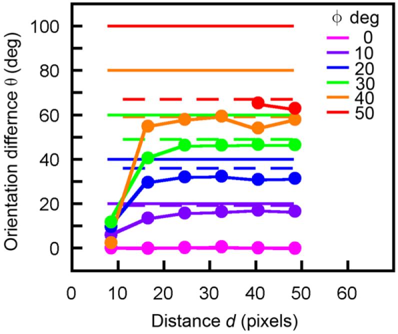
Orientation difference as a function of the distance and direction of one edge element from another. The symbols show the most likely orientation differences for edge elements of natural contours (from the upper quadrant of Fig. 6b; see also Fig. 7a). The solid horizontal lines show the predictions if the most likely relationship were cocirular. The horizontal dashed line show the predictions if the most likely relationship were parabolic.

Another hypothesis for contour grouping (and interpolation) is based on the definition of “relatable” contours: Two edge elements are relatable if their linear extensions (toward each other) intersect and if the outer angle of their intersection is acute (Shipley & Kellman 1991; Kellman 2003). The range of relatable orientation differences decreases as a function of direction so that for a direction near 0 deg the range of relatable orientation differences is 0-90 deg and for a direction of 50 deg the range of relatable orientation differences is 50-90 deg (see Supplementary Fig. 1). Our measurements of natural contours show that many natural contours are not relatable and that many relatable contours are unlikely to occur in natural scenes (see Fig. 7a). Our measurements of (naïve) human performance in the natural contour occlusion task show that human decisions closely match the natural scene statistics; thus, humans do not perceptually link many edge element pairs that are relatable, and they do perceptually link many contour element pairs that are not relatable.

Interestingly, the statistics of natural contours are roughly consistent with a parabolic relationship. If the most likely element orientation difference θ has a parabolic relationship to the reference element (with the origin of the parabola tangent to the reference element), then the highest-likelihood orientation difference would be tan^-1 (2 tan ϕ), independent of the distance d.

The horizontal dashed lines in Fig. 13 show the predictions of a parabolic relationship. However, it is important to keep in mind that this only summarizes the highest-likelihood orientation difference in each distance and direction bin; whereas human performance in our task depends on the entire likelihood distribution.

The approximately parabolic relationship between edge elements in natural images also holds for the within domain statistics in Fig. 5c (which also undoubtedly reflect the shape properties of contours). This finding supports the validity of the hand-segmentation method used to obtain the across-domain statistics.

Singh & Fulvio (2005; 2007) had observers extrapolate smooth contours across half-disk occlusion regions. They varied the disk diameter and inducing contour shape. Observers set the direction and orientation of the test edge element to smoothly extrapolate the inducing contour. They found that observers extrapolate contours with a bias toward decreasing curvature with increasing distance, a bias more consistent with parabolic than circular contours. Their result is therefore qualitatively consistent with our natural scene statistics and with our observer’s performance in the natural contour occlusion task.

The finding of an approximately parabolic statistical relationship between the edge elements of natural contours implies that natural contours tend not to be circular in shape, but the finding does not imply that contours tend to be parabolic in shape. Recall that all elements on a contour serve as the reference (not just the elements at points of highest curvature) and that both edge elements in each pair-wise comparison serve as the reference element. If natural contours tend to be circular in shape then no matter which elements serve as the reference, one would expect a co-circular relationship rather than the parabolic relationship in Fig. 5c and 6b. On the other hand, the observed parabolic relationship is not related to any particular simple underlying shape. Rather, it is a purely statistical result that undoubtedly depends on the fact that most natural contours contain random changes in curvature, including changes in the sign of the curvature (i.e., inflection points). Thus, no matter where one starts on a contour, if a contour element at some distance from the starting element happens to end up in a different direction from the direction pointed to by the orientation of the starting element, then its orientation (because of the distribution of random changes in curvature) ends up on average in a parabolic relationship with the starting element. Our psychophysical results suggest that humans use knowledge of this parabolic relationship (and the appropriate range around it) to decide whether or not to link contours passing under an occluding surface. We also note that even though humans may know that most natural contours tend to randomly change in curvature and to have one or more inflection points, they probably choose to make smooth monotonic interpolations (when forced to do so) because they generally have no information that would allow them to select specific points behind the occluding surface for an inflection or rapid change in curvature. Of course, in cases with convincing information (e.g., a very wiggly contour exiting both sides of the occluding surface) they would probably make less smooth non-monotonic interpolations.

Contour integration

Another useful task for investigating the mechanisms of contour grouping over extended distances is the contour integration task (Beck et al. 1989; Field et al. (1993); Kovaks & Julesz 1993). In this task, the signal-plus-noise stimulus consists of an extended contour defined by discrete contour elements embedded in a background of random contour elements; the noise stimulus consists of only random contour elements. The subject’s task is to detect the embedded contour. Much has been learned about the mechanisms of contour grouping by manipulating specific properties of the embedded contour elements relative to those of the background elements. The contour integration task is very useful because when the stimuli are properly designed, the embedded contour can be only detected if the visual system contains mechanisms that group contour elements using the specific properties of interest. Our measured natural contour statistics are potentially relevant to a number of the studies using the contour integration task, but we mention just two here.

In our earlier study, we measured detection performance for line-segment contours embedded in line-segment backgrounds (Geisler et al. 2001; see also Tversky et al. 2005). Parametric data was obtained for a number of embedded contour properties: contour length, contour shape, and contour element orientation jitter (orientation noise). Based on a somewhat different characterization of the across-domain contour statistics described here, we proposed a single-parameter model of performance in the contour integration task. That model did not take into account the contrast polarity dimension and used a less well-defined version of the ideal decision rule for pair-wise contour element grouping (compare the current eq. (2) with eq. (1) and (2) in Geisler et al. 2001). We have generated predictions for the earlier contour integration task, using the characterization of the contour statistics in Fig. 6 and the current eq. (2). Specifically, the model assumes the observer first links together all line segments in the display that satisfy eq. (2), then forms larger groups by transitive grouping (i.e., finds those groups of line segments that are linked to each other either directly or through unbroken links to other elements), and finally selects the stimulus interval containing the longest group (for more details see Geisler et al. 2001). The version of this model observer that uses both the likelihoods and the distant-dependent decision criterion (Fig. 7b) performs poorly in the contour integration task, much poorer than the human observers. However, the version of this model that uses a fixed decision criterion of 1.0 (Fig. 7a) performs well in the contour integration task and its performance correlates well with human observer performance (r = 0.88).

This is a surprising result because in the contour integration task the prior probability of a pair of contour elements belonging to the same contour falls rapidly with distance (as in natural scenes). Apparently, ignoring the pair-wise priors that would be appropriate for a simple contour occlusion task (with natural priors) yields an effective heuristic for grouping extended contours. It is important to note, however, that the true ideal observer for the contour integration task is unknown, and thus it is also unknown how close our model observer approaches ideal performance. Also, in exploring the class of contour integration models that have a fixed decision criterion over distance we discovered that it is possible to maintain nearly equivalent good performance by trading off the radius over which the initial pair-wise edge linking occurs with the value of the fixed decision criterion—the larger the radius the larger the value of the decision criterion.

Field, Hayes and Hess (2000) conducted contour integration experiments where the phase (contrast polarity) of the contour elements was either maintained or alternated along the embedded contour. They found that contour detection performance was substantially reduced when contrast polarity was alternated. Our measurements of natural contour statistics show that when contrast polarity reverses a rational observer should apply a more stringent criterion for integrating the contour elements. Although we have not derived specific predictions for the Field et al. stimuli, we have shown that applying a more stringent criterion (the left half of Fig. 7a) produces a substantial drop in contour integration performance. Thus, their findings are at least qualitatively consistent with the hypothesis that humans are basing their decisions on the average statistical properties of natural contours.

Natural systems analysis

The study described in this article is representative of a new approach to perceptual neuroscience that has been emerging in recent years. This approach, which might be termed “natural systems analysis,” consists of several components. The first is to identify and characterize a natural task or natural sub-task that is performed by the organism under natural conditions. In our case, this is the contour occlusion task (see Fig. 1). The second component is to measure and analyze those specific environmental properties (natural scene statistics) relevant for performing the task. Usually, these would be across-domain statistics such as the pair-wise contour statistics described in Fig. 6. The third component is a computational analysis to determine how a rational (ideal) perceptual system would exploit the measured environmental properties to perform the natural task. This component is critical because it provides insight into the information contained in the natural stimuli and it can suggest principled hypotheses for the neural mechanisms the organism might use to exploit that information. The fourth component is to formulate specific hypotheses for neural mechanisms (based on the first three components) and test them in physiological and/or behavioral studies that capture the essence of the natural task. In our case, the hypotheses were based on the optimal grouping rules derived from the natural scene statistics (Fig. 7a), and the behavioral studies used a simplified contour occlusion task where the stimuli were constructed directly from natural images (Fig. 4). The study described here is unusual in that it involves all four components of a natural systems analysis, but that is not particularly important. What is important is the growing realization among perception researchers that the perceptual systems must reflect the tasks the organism performs and the statistical properties of the stimuli it uses to perform those tasks. Studies that take this realization to heart are more likely to produce significant advances in behavioral and systems neuroscience.

Appendix

Here we show that the decision rule in equation (1) is equivalent to the one in equation (2).

From the definition of conditional probability:

$$\frac{p(c=1\mid d,\varphi ,\theta ,\rho )}{p(c=0\mid d,\varphi ,\theta ,\rho )}=\frac{p(c=1,d,\varphi ,\theta ,\rho )}{p(c=0,d,\varphi ,\theta ,\rho )}=\frac{p(\varphi ,\theta ,\rho \mid c=1,d)p(c=1\mid d)p\left(d\right)}{p(\varphi ,\theta ,\rho \mid c=0,d)p(c=0\mid d)p\left(d\right)}$$

and thus,

$$\frac{p(c=1\mid d,\varphi ,\theta ,\rho )}{p(c=0\mid d,\varphi ,\theta ,\rho )}=\frac{p(\varphi ,\theta ,\rho \mid c=1,d)p(c=1\mid d)}{p(\varphi ,\theta ,\rho \mid c=0,d)p(c=0\mid d)}$$

It follows that

$$p(c=1\mid d,\varphi ,\theta ,\rho )>p(c=0\mid d,\varphi ,\theta ,\rho )$$

if and only if

$$\frac{p(\varphi ,\theta ,\rho \mid d,c=1)}{p(\varphi ,\theta ,\rho \mid d,c=0)}>\frac{p(c=0\mid d)}{p(c=1\mid d)}$$

References

- Barrow HG, Tenebaum JM. Computational approaches to vision. In: Boff KR, Kaufman L, Thomas JP, editors. Handbook of Perception and Human Performance, Volume II: Cognitive Processes and Performance. John Wiley and Sons; New York: 1986. pp. 38pp. 31–38.pp. 68 [Google Scholar]
- Beck J, Rosenfeld A, Ivry R. Line segregation. Spatial Vision. 1989;4:75–101. doi: 10.1163/156856889x00068. [DOI] [PubMed] [Google Scholar]
- Brunswik E, Kamiya J. Ecological cue-validity of ‘proximity’ and other Gestalt factors. American Journal of Psychology. 1953;66:20–32. [PubMed] [Google Scholar]
- Elder JH, Goldberg RM. Ecological statistics of Gestalt laws for the perceptual organization of contours. Journal of Vision. 2002;2:324–353. doi: 10.1167/2.4.5. [DOI] [PubMed] [Google Scholar]
- Feldman J. Bayesian contour integration. Perception & Psychophysics. 2001;63(7):1171–1182. doi: 10.3758/bf03194532. [DOI] [PubMed] [Google Scholar]
- Field DJ, Hayes A, Hess RF. Contour integration by the human visual system: Evidence for a local ‘association field’. Vision Research. 1993;33:173–193. doi: 10.1016/0042-6989(93)90156-q. [DOI] [PubMed] [Google Scholar]
- Field DJ, Hayes A, Hess RF. The role of polarity and symmetry in perceptual grouping of contour fragments. Spatial Vision. 2000;13:51–66. doi: 10.1163/156856800741018. [DOI] [PubMed] [Google Scholar]
- Geisler WS. Visual perception and the statistical properties of natural scenes. Annual Review of Psychology. 2008;59:10.11–10.26. doi: 10.1146/annurev.psych.58.110405.085632. [DOI] [PubMed] [Google Scholar]
- Geisler WS, Perry JS, Super BJ, Gallogly DP. Edge co-occurrence in natural images predicts contour grouping performance. Vision Research. 2001;41:711–724. doi: 10.1016/s0042-6989(00)00277-7. [DOI] [PubMed] [Google Scholar]
- Geisler WS, Perry JS, Ing AD. Natural systems analysis. In: Rogowitz B, Pappas T, editors. Human Vision and Electronic Imaging, SPIE Proceedings; 2008.p. 6806. [Google Scholar]
- Grossberg CM, Mingolla E. Neural dynamics of form perception: Boundary completion, illusory figures, and neon color spreading. Psychological Review. 1985;92(2):173–211. [PubMed] [Google Scholar]
- Kellman PJ. Interpolation processes in the visual perception of objects. Neural Networks. 2003;16:915–923. doi: 10.1016/S0893-6080(03)00101-1. [DOI] [PubMed] [Google Scholar]
- Kellman PJ, Shipley TF. A theory of visual interpolation in object perception. Cognitive Psychology. 1991;23:141–221. doi: 10.1016/0010-0285(91)90009-d. [DOI] [PubMed] [Google Scholar]
- Kovacs I, Julesz B. A closed curve is much more than an incomplete one: Effect of closure in figure-ground segmentation. Proceedings of the National Academy of Sciences. 1993;90:7495–7497. doi: 10.1073/pnas.90.16.7495. [DOI] [PMC free article] [PubMed] [Google Scholar]
- Martin D, Fowlkes C, Malik J. Learning to detect natural image boundaries using local brightness, color and texture cues. IEEE Transactions on Pattern Analysis and Machine Intelligence. 2004;26:530–549. doi: 10.1109/TPAMI.2004.1273918. [DOI] [PubMed] [Google Scholar]
- Neumann H, Mingolla E. Computational models of spatial integration in perceptual grouping. In: Shipley TF, Kellman PJ, editors. From fragments to objects: Grouping and segmentation in vision. Elsevier; Amsterdam: 2001. pp. 353–400. [Google Scholar]
- Parent P, Zucker S. Trace inference, curvature consistency and curve detection. IEEE Transactions on Pattern Analysis and Machine Intelligence. 1989;11:823–839. [Google Scholar]
- Rock I. An introduction to perception. Macmillan; New York: 1975. [Google Scholar]
- Sha’ashua S, Ullman S. Structural saliency: The detection of globally salient structures using a locally connected network; Proceedings of the Second International Conference on Computer Vision; 1988.pp. 321–327. [Google Scholar]
- Sigman M, Cecchi GA, Gilbert CD, Magnasco MO. On a common circle: Natural scenes and Gestalt rules. Proc. National Academy of Science. 2001;98:1935–1940. doi: 10.1073/pnas.031571498. [DOI] [PMC free article] [PubMed] [Google Scholar]
- Singh M, Fulvio JM. Visual extrapolation of contour geometry. PNAS. 2005;102(3):939–944. doi: 10.1073/pnas.0408444102. [DOI] [PMC free article] [PubMed] [Google Scholar]
- Singh M, Fulvio JM. Bayesian contour extrapolation: Geometric determinants of good continuation. Vision Research. 2007;47:783–798. doi: 10.1016/j.visres.2006.11.022. [DOI] [PubMed] [Google Scholar]
- Tversky T, Geisler WS, Perry JS. Contour grouping: Closure effects are explained by good continuation and proximity. Vision Research. 2004;44:2769–2777. doi: 10.1016/j.visres.2004.06.011. [DOI] [PubMed] [Google Scholar]
- Ullman S. Filling-in the gaps: The shape of subjective contours and a model for their generation. Biological Cybernetcs. 1976;25:1–6. [Google Scholar]
- Wertheimer M. Principles of perceptual organization. In: Beardslee DC, Wertheimer M, editors. Readings in Perception. Van Nostrand; Princeton: 1958. pp. 103–123. Original work published 1923. [Google Scholar]
Associated Data
This section collects any data citations, data availability statements, or supplementary materials included in this article.