A single-sample method for normalizing and combining full-resolution copy numbers from multiple platforms, labs and analysis methods

Abstract

Motivation: The rapid expansion of whole-genome copy number (CN) studies brings a demand for increased precision and resolution of CN estimates. Recent studies have obtained CN estimates from more than one platform for the same set of samples, and it is natural to want to combine the different estimates in order to meet this demand. Estimates from different platforms show different degrees of attenuation of the true CN changes. Similar differences can be observed in CNs from the same platform run in different labs, or in the same lab, with different analytical methods. This is the reason why it is not straightforward to combine CN estimates from different sources (platforms, labs and analysis methods).

Results: We propose a single-sample multi source normalization that brings full-resolution CN estimates to the same scale across sources. The normalized CNs are such that for any underlying CN level, their mean level is the same regardless of the source, which make them better suited for being combined across sources, e.g. existing segmentation methods may be used to identify aberrant regions. We use microarray-based CN estimates from ‘The Cancer Genome Atlas’ (TCGA) project to illustrate and validate the method. We show that the normalized and combined data better separate two CN states at a given resolution. We conclude that it is possible to combine CNs from multiple sources such that the resolution becomes effectively larger, and when multiple platforms are combined, they also enhance the genome coverage by complementing each other in different regions.

Availability: A bounded-memory implementation is available in aroma.cn.

Contact: hb@stat.berkeley.edu

1 INTRODUCTION

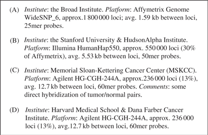
The Cancer Genome Atlas (TCGA) project (Collins and Barker, 2007; TCGA Network, 2008) is a collaborative initiative to better understand cancer using existing large-scale whole-genome technologies. One of the tumor types studied is brain cancer, more precisely glioblastoma multiforma (GBM). GBM is a fast growing tumor, where the survival rate is low and the life expectancy after diagnosis is on average 14 months. One objective of TCGA is to identify copy number (CN) aberrations and polymorphisms in GBM samples. Within TCGA, there is a set of Tissue Collection Centers (TCCs) that collects and stores tissues from GBM patients. To date, tumor and normal tissues (or blood) from more than 200 individuals have been collected. Each TCC sends tissues and clinical metadata to the TCGA Biological Collection Resource (BCR), which in turn provides the different TCGA centers with prepared biospecimen analytes (DNA and RNA) for further analysis. In Table 1, the four TCGA centers that conduct CN analysis on GBM samples are listed. They are all using different DNA microarray technologies. The CN results generated by these centers are sent to the TCGA Data Coordinating Center (DCC) and published online. A large number of samples are analyzed at more than one site, but not all. More details on the TCGA organization and work flow can be found in the Supplementary Materials of TCGA Network (2008).

Table 1.

Summary of CN datasets (sources) listing the name of the participating institute (TCGA center), the platform used, the number of CN estimates produced and additional comments.

Thus far the different TCGA centers have identified CN regions independently of each other. It has been suggested that more accurate and precise results at a higher resolution and with greater coverage could be obtained if the CN estimates from the different sites are combined. The data can be combined at various levels, e.g. at the level of full-resolution CNs (Bengtsson et al., 2008b) and at the level of segmented CN regions. It can be argued that combining the data at the full resolution will leave more options for choosing downstream methods.

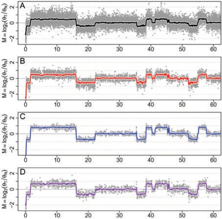
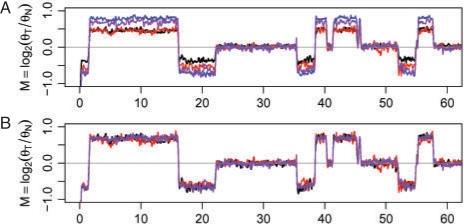
The main differences observed when comparing CN estimates originating from different labs, platforms and preprocessing methods are that: (i) the mean levels of CN aberrations differ, and (ii) the noise levels differ at the full resolution. This is illustrated in Figure 1, which shows CN estimates for one sample in a particular region. Although the different CNs from the four sources show very similar CN profiles, it is clear that the attenuation and the noise levels differ (cf. Ylstra et al., 2006). See also Figure 2A. Other notable differences are that the platforms have (iii) different numbers of loci, and (iv) varying coverages in different parts of the genome. We will later also see that (v) the relationships between platforms are often non-linear.

Fig. 1.

Full resolution and smoothed tumor/normal CNs in a 60 Mb region on Chr 3 of TCGA sample TCGA-02-0104 as measured by four different labs based on three different types of microarray SNP and CN platforms (Table 1). The full-resolution estimates are displayed as light points and the smoothed estimates, which are available at every 100 kb, are displayed as dark colored curves. For set A there are 88 000 full-resolution CNs on Chr 3, for set B there are 38 000 CNs, and for sets C and D there are 15 000 CNs (approximately).

Fig. 2.

Smoothed tumor/normal CNs before (A) and after (B) multisource normalization. The same region as in Figure 1 is depicted (with a different vertical scale).

In this article, we present a normalization for full-resolution CN estimates from multiple sources (abbreviated MSCN) which ensures that the observed mean estimates for any true CN level agree across sources such that there is a linear relationship between sources. The method is applied to each sample independently, and requires only raw CN ratios or log-ratios. Calibration toward known CN levels can be applied afterward and is not considered here. For CN signals based on SNP probes, it is only total CN estimates that are normalized; relative allele signals (‘raw genotypes’) are left unchanged.

The realization of a single-sample method has several implications: (i) Each sample can be processed as soon as CN estimates from the different sources are available. (ii) Samples can be processed in parallel on different hosts/processors making it possible to decrease the processing time of any dataset linearly with the number of processors. (iii) There is no need to reprocess a sample when new samples are produced, which further saves time and computational resources. Furthermore, (iv) the decision to filter out poor samples can be made later, because a poor sample will not affect the processing of other samples. More importantly, a single-sample method is (v) more practical for applied medical diagnostics, because individual patients can be analyzed at once, even when they come singly rather than in batches. This may otherwise be a limiting factor in projects with a larger number of samples.

Although it might appear possible, the data and results presented here cannot and should not be used to compare platforms, labs or algorithms. Such comparisons require precisely defined objectives, which will vary with the underlying biological question or hypothesis. With appropriately defined objectives, an evaluation method could be designed, and then such comparisons could be made. At the moment, we are taking the CN estimates from the different platforms as they are given to us; we do not even know at this point whether they are all optimized to achieve the same objective. As a result, comparisons of the kinds mentioned are beyond the scope of this article, although they are definitely of interest to us, and we hope to carry them out in the future.

The outline of this article is as follows. In Section 2, we give our definitions of the terms calibration and normalization, and describe the model and algorithm for the normalization method. In Section 3, we show that the normalized CNs across sources are proportional to each other, which is a necessary property. At the end, we illustrate how the combined normalized CN estimates increase the power to detect change points, in comparison with the separate sources, and combined, un-normalized CN estimates. In Section 4, we conclude the study, discuss potential limitations, call for extended segmentation methods and give future research directions.

2 METHODS

2.1 Dataset

For this study, we used data from the TCGA project. From the DCC data portal, we downloaded (May and June 2008) Level 2 CN estimates for GBM tumors and normal blood/normal tissues for 60 individuals that have estimates from all four sources. For the purpose of illustrating our method, we will focus mainly on sample TCGA-02-0104 (vials 01A versus 10A), because it has a large number of CN aberrations on Chr 3 at different mean levels. For the evaluation, we will use samples TCGA-06-0178 (01A versus 10B) and TCGA-02-0026 (01B versus 10A). We have found that the normalization method works equally well in other regions as well as with other samples (data not shown).

2.1.1 Copy numbers

Although not restricted to such, all CN estimates used here are log-ratio CNs calculated as:

(1)

where θ_i,j is the non-polymorphic signal at locus j=1,…, J for sample i=1,…, I and θ_R,j is the corresponding reference (R) signal. Where allele-specific estimates (θ_i,j,A, θ_i,j,B) are provided, the non-polymorphic signals are calculated as θ_i,j=θ_i,j,A+θ_i,j,B. In this study the reference signals are from the normal target DNA in the tumor/normal pair. In non-paired studies, the reference is often calculated as the robust average across a pool of samples, (cf. Bengtsson et al., 2008b). We note that the proposed method could also be applied to CN ratios before taking logarithms.

2.1.2 Direct and indirect CN ratios

Due to the nature of the platforms, the Affymetrix and Illumina tumor/normal CNs are indirect in silico ratios of signals originating from two hybridizations. The Agilent platform is a two-color assay where two DNA targets are co-hybridized to the same microarray. Some of the tumor/normal pairs from Source C come from direct co-hybridizations of tumor and normal samples, while the majority from Source C and all from Source D come from two hybridizations: one in which the tumor sample is co-hybridized with a common DNA reference (Promega Reference DNA). Ideally the common reference channels (approximately) cancel out when calculating the ratios (of ratios). The two TCGA-02 samples were hybridized directly at Source C.

2.2 Proposed model

The proposed MSCN was designed to: (i) be applicable to CN estimates from a wide range of technologies including, but not exclusively, microarrays, (ii) provide full-resolution normalized estimates and (iii) normalize each sample independent of the others. As explained in the Section 1, there are several advantages of a method that can be applied to one sample at a time compared with one that requires multiple samples.

2.3 Normalization model

Sources s=1,…, S provide CN estimates at different (possibly non-overlapping) sets of loci. Dropping sample index i in what follows, let y_s,j denote the CN estimate from source s at genomic position x_j, where these will be specific to the source, though possibly overlapping. Let μ_j denote the underlying true but unknown CN at the corresponding locus. For y_s,j, we will here use the CN log-ratio M_j from source s. In Figure 1 four different sets of (un-normalized) CN estimates for the same sample are shown for a common region on Chr 3.

2.3.1 Non-linear measurement functions

We model the observed (estimated) CNs {y_s,j} as:

(2)

where f_s(·) is a source-specific function and ε_s,j is source-specific noise. This measurement function (Bengtsson and Hössjer, 2006) for source s encapsulates how the signals of interest are transformed by the platform and the data processing. We assume that f_s(·) is smooth and strictly increasing.

An important and necessary assumption made in Equation (2) is that the measurement function is independent of the true CN level. Previous studies indicate that this may not be true when an inappropriate preprocessing method is used for estimating CN ratios (Bengtsson and Hössjer, 2006). If this is the case, we assume the effect is approximately the same across sources, and if it is not, we assume the effects are small enough to be ignored.

2.3.2 Calibration

Consider the case where the true CN is known for a set of loci, and that the CNs for these loci are reasonable spread out (have wide support). Regression techniques can then be used to estimate f_s(·) based on the subset of {(μ_j, y_s,j)} for which the truth is known. Backtransformation gives an estimate of the true CN as:

(3)

where f⁻¹_s(·) is referred to as the calibration function. One of the properties of a calibration function is that the calibrated signals (here denoted ) are proportional to the true signals.

2.3.3 Normalization

However, here we will consider the much more common case where the truth is not available, especially not at a range of CN levels. Instead of calibration functions, we will estimate normalization functions {h⁻¹_s(·)}, which, when used in place of in Equation (3), backtransform signals such that the signals effectively get the same measurement function afterwards, i.e. the normalized signals are on the same scale. To be more precise, we will estimate {h⁻¹_s(·)} such that when full-resolution CNs are transformed as:

(4)

we obtain

(5)

where is a measurement function common to all sources. Although this measurement function is still unknown, we know that it is the same for all sources. This means that, after normalization there will be an approximately proportional (linear) relationship between the sources. In other words, with zero-mean noise, the means of the normalized CNs are the same when the true CN μ_j=μ. This is a property required by most segmentation methods and other downstream methods. For a further discussion on calibration and normalization, see Bengtsson (2004) and Bengtsson and Hössjer (2006).

2.3.4 Estimating normalization functions

In Bengtsson and Hössjer (2006) and Bengtsson et al. (2004) the authors proposed affine (‘linear’) models for normalizing and calibrating multidimensional signals, respectively. In both cases, principal component analysis (PCA) techniques were used to estimate linear subspaces of data to infer the normalization (calibration) functions. We will generalize those models and algorithms in two ways. First, in order to account for the fact that the sources estimate CNs at different loci, we generate CN estimates at a common set of loci using kernel estimators. Second, in order to model non-linear relationships between sources we utilize principal curves (Hastie and Stuetzle, 1989).

2.3.5 Constructing CN estimates at a common set of loci

In order to estimate the normalization functions, we need a complete set of CN estimates at a large number of loci. Because different sources produce CNs at different loci, we estimate CNs at a predefined set of target loci from CNs available in the proximity of each target locus. Here, the set of target loci will consist of every 100 kb locus throughout the genome. Note that the choice of locations is not critical. More precisely, for target locus j with position x_j we construct CN estimates {z_s,j} for all sources by utilizing kernel estimators as follows. For each source s and target locus j, calculate:

(6)

where {w_j,j′≥0} are weights with constraint ∑_j′ w_j,j′=1;

(7)

with Φ(·) being the Gaussian density function and σ a bandwidth parameter. Mainly for computational efficiency, but also for robustness, we choose to truncate the kernel at |x_j′−x_j|>3σ (excluding 0.27% of the density) by giving such data points zero weight. We ignore potential bias problems at the extreme locations. Moreover, if there are no data points within the truncated window for one of the sources, we treat that as a missing value and ignore that target locus. Note, by inserting Equation (2) in Equation (6), we obtain

(8)

where ε′_s,j=∑_j′ w_j,j′ ε_s,j′. Next, by assuming that (i) the underlying true CN is locally constant, which is reasonable to believe except for positions close to change points, and that (ii) the function f_s(·) is approximately linear in this range, we can approximate the above with:

(9)

In the latter step we used the fact that if the true CN is locally constant, then ∑_j′ w_j,j′ μ_j′=μ_j, with the equality being replaced by an approximation when change points are taken into account. Bias due to change points can to some extent be controlled for by replacing Equations (6) and (7) with a robust kernel estimator, and partly by using a truncated kernel (as above). Finally, comparing Equation (2) with Equation (9), we see that the smoothed estimates {z_s,j} and the original estimates {y_s,j} have undergone (approximately) the same transformation via f_s(·). Thus, we can use {z_s,j} as a proxy for the incomplete {y_s,j} to estimate normalization functions. We want to emphasize that the above smoothed estimate of CN are only used for estimating the normalization functions; it is the original full-resolution data that will be normalized.

2.3.6 Relationship between sources

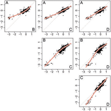
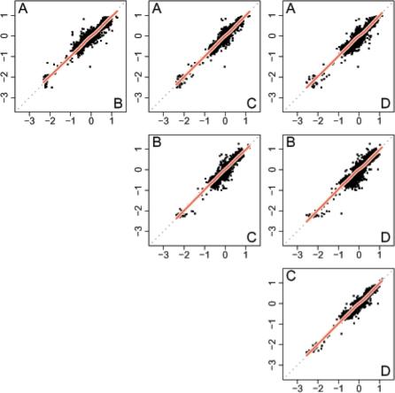
From Equation (9), we expect {(z_1,j,…, z_S,j)} to scatter around the one-dimensional curve f(μ)=(f₁(μ),…, f_S(μ)) in S dimensions, where μ is the true CN. This is confirmed by the different pairs {(z_s,j, z_t,j)} plotted in Figure 3. It is clear that the ‘sensitivity’ (amplitude of the estimates) differ between sources, e.g. the absolute values from Source C are greater than Source A. Although these relationships are similar across samples, we find that they are not similar enough in order to reuse their estimates across sources. There are even cases where they are reversed (data not shown). These plots also show that the relationship between two sources is not linear but slightly non-linear, especially at ‘extreme’ CN levels. This indicates that at least one of the underlying measurement functions are non-linear. There exist various reasons for this non-linearity, where offset (Bengtsson and Hössjer, 2006) and saturation (Ramdas et al., 2001) in probe signals are two.

Fig. 3.

Smoothed CNs for the six different pairs of sources. Data from all autosomal chromosomes in one individual is displayed. Each curve depicts the overall pairwise relationship between the two datasets plotted. These curves, which are used only to illustrate the relationships, are fitted using smooth splines with five degrees of freedom.

2.3.7 Potential problems with Chr X and Chr Y estimates

From looking at 60 tumor/normal pairs, we have concluded that there exists a common across-locus relationship between any two sources. However, for estimates on sex chromosomes we have observed that the estimated CNs do not necessarily follow the same trend, at least for some of the data sources (data not shown). We believe this is because some preprocessing methods post-curate CN estimates from Chr X and Chr Y in order to control for differences in males and females, and the corrections differ with methods. For this reason, we fit the normalization functions using signals only from autosomal chromosomes. For the practical purpose of normalizing and combining Chr X and Chr Y data, we suggest that one studies the pairwise relations for these chromosomes carefully. If it is clear from looking at multiple samples that one source is curating the data in such a way that the relationship cannot be estimated and backtransformed, then one may want to exclude its Chr X and Chr Y CNs from the combined dataset, or if possible, use an alternative preprocessing method for estimating CNs.

2.3.8 Estimating normalization functions

When the measurement functions are linear, we can use techniques from principal component analysis to estimate a one-dimensional line h(λ)=(h₁(λ),…, h_S(λ))∈ℝ^S from {(z_1,j,…, z_S,j)}. However, since the measurement functions here are non-linear, we instead use a related technique based on principal curves (Hastie and Stuetzle, 1989). This allows us to estimate a one-dimensional curve h(λ)=(h₁(λ),…, h_S(λ))∈ℝ^S based on {(z_1,j,…, z_S,j)}. As argued above, we cannot regress on the true CNs {μ_j}, because they are unknown. For this reason, we can only parameterize h(·) modulo the unknown relationship . A natural constraint is to parameterize such that is strictly monotone. This will avoid sign swaps, which is a common problem whenever using PCA-based techniques. We use the algorithm suggested by Hastie and Stuetzle (1989), which is implemented in the princurve package (Weingessel and Hastie, 2007), for estimating principal curves. This method can be robustified by using iterative re-eighted least squares (IRWLS) methods, (cf. Bengtsson et al., 2004). We define the normalization functions to be the inverse of the individual components of the estimated principal curve, that is, , such that is an estimate of by source s.

2.3.9 Normalizing toward a target source

In addition, or as an alternative to the above constraint, one option is to constrain the principal curve, or alternatively the normalization function, such that the normalized data will be on the same scale as one of the sources, which is then referred to as the target source. This is done by forcing the corresponding normalization function to equal the identity function. For instance, h₁(λ)=λ keeps CNs for the first source unchanged. This is a natural way to parametrize the curve uniquely. This strategy is also useful in the case where CNs from one source are known to be more consistent across samples than CNs from other sources. This more stable target source will then be used to control for across-sample variations. For similar reasons, in the case where there is only one source that produces estimates for all samples, then that source can used as the target source. Moreover, if the target source produces calibrated CNs, that is, CNs that are proportional to the true CNs, then the normalized CNs for all other sources will become calibrated as well.

2.3.10 Applying normalization functions

Finally, with estimates of {h⁻¹_s(·)}, we normalize the observed full-resolution CNs as:

(10)

with being referred to as the (full-resolution) multisource normalized CNs. Coupled with each normalized dataset is an overall variance σ²_s, which can be estimated from using for instance a robust first-order difference variance estimator (Korn et al., 2008; von Neumann et al., 1941).

2.3.11 Combining full-resolution normalized CNs

The normalized CNs may be combined by merging (interweaving) them across sources generating a new set denoted by , which is the joint set of CNs from all sources. The normalized and merged CN estimates are likely to be heteroscedastic, because the noise levels (σ²_s) differ between sources. Other sources of variation, such as locus-specific error terms, may add to the heteroscedasticity as well. In the following section, we will give one example on how the heteroscedasticity can be modeled using locus-specific weights that are proportional to 1/σ²_s.

2.4 Evaluation

Although different CN studies have different objectives, an important one is to segment the genome into regions that reflect the underlying piecewise constant nature of the true CNs. The main strategy of many segmentation methods is to identify the change points, and then estimate the mean CN levels between change points. Consider the case where there exist only one change point in a specific region and that the location of it is known. This region may be defined by two flanking change points and/or the chromosome ends. Then, under the above assumptions, the ability to detect this change point is determined mainly by: (i) the magnitude of change in the (observed) CNs, (ii) the noise level of the CNs and (iii) the distance (and/or the number of data points) to the left and the right of the change point. Depending on model, for instance the t-test can be used to test whether there exist a change point or not at the given locus (Page, 1955). Given such a test for a fixed locus, when the location of the change point is unknown, one can scan the region for the locus that gives the highest score above some required significance threshold. To test for multiple change points, several strategies have been suggested, e.g. using a recursive divide-and-conquer approach to identify a new change point in the region defined by two existing change points (Venkatraman and Olshen, 2007). Since a large number of loci are scanned and many change points are identified, correction for multiple testing is needed.

The evaluation method used here is inspired by the fundamentals of the above test without having to rely on a specific segmentation method. First, we pick a region in one sample for which there is strong evidence that there exist only one change point (which is in the center of the region). For each dataset s, we then identify the sets of loci in this region that are to the left and to the right of the change point. We exclude loci that are within 500 kb of the change point for robustness against errors in the location of the change point.

Since the comparison of datasets has to be done on the same ‘resolution’, we construct a new set of common estimates by binning the CNs in non-overlapping windows of equal (physical) lengths h and averaging within each window. This corresponds to using a uniform kernel of width h in Equation (6) and apply it to every h position. Note that this approach is guaranteed to use all available data points. Here, we use a weighted median estimator with weights such that data points from more noisy sources have less impact on the smoothed estimate. Let and denote the resulting smoothed CNs for the left and the right set of loci in dataset s. Next, we use receiver operating characteristic (ROC) analysis (Bengtsson et al., 2008b) to assess how well these two subsets of smoothed CNs separate the CN states defined by the two sides of the change point. We argue that this is related to how a segmentation method tests for a change point.

2.5 Algorithm and implementation

The MSCN method is available in R (R Development Core Team, 2008) package aroma.cn part of the aroma.affymetrix framework (Bengtsson et al., 2008a). The method is designed and implemented to have bounded-memory usage, regardless of the number of samples/arrays processed. Furthermore, the complexity of the algorithm is linear in the number of loci (J), and linear or near linear in the number sources (S). Since it is a single-sample method, the samples can be preprocessed in parallel on multiple hosts/processors. The method applies to any type of technology.

3 RESULTS

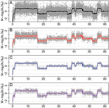
The result from applying MSCN to observed TCGA-02-0104 tumor/normal CNs is shown in Figure 4. After normalization, the full-resolution data are such that the mean levels of the different CN regions are the same for all sources. This can be seen if comparing the smoothed CNs (i) along the genome (Fig. 2B), and (ii) between pairs of sources (Fig. 5). This shows that the normalized estimates of CNs have the property defined by Equation (5).

Fig. 4.

Normalized full-resolution tumor/normal CNs in the same sample and region as in Figure 1. Source D was used as the target source, which is why the estimates from that source does not change.

Fig. 5.

Smoothed normalized CNs for the six different pairs of sources. After normalization the relationship between sources is approximately linear. The sample and loci shown are as in Figure 3.

3.1 Better CN separation at a given resolution

Here, we assess how well various CN estimates in the same region can differentiate between two (unknown) CN states using the method described in Section 2.4. For this purpose, we use two regions in two different samples. The first is a 43.2 Mb region around a change point at Chr10:114.77 Mb in sample TCGA-06-0178, and the second is a 13.0 Mb region around a change point at Chr12:28.0 Mb in sample TCGA-02-0026. The CN change is greater for the latter change point. As the MSCN is a single-sample method, these two samples were normalized (MSCN) and evaluated independently of each other.

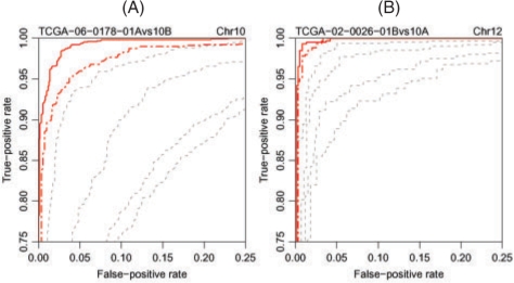
In Figure 6, the ROC performances of the combined normalized and un-normalized CNs as well as each of the individual sources are depicted for these regions. For the two regions we smoothed the CNs in bins of size h=25 kb and h=15 kb, respectively. First, we note that when combining sources, the normalized CNs separate the two CN state better than the un-normalized data. This is because the inter-locus variability due to differences in mean levels, which in turn is due to the non-linear relationships between sources, is removed. From the pairwise relationships in Figure 3, we observe that the discrepancy between mean levels is larger for the more extreme CN levels. For this reason, we also expect the inter-locus variability to be greater at these levels, making the normalization even more important. We also note that the combined normalized CNs perform better than any of the individual sources. This is because there are more data points available within each window providing more precise estimates of the underlying true CN. For similar reasons, and because of differences in noise levels (of the smoothed data), we observe different performances across sources. Since there is a risk that false conclusions are drawn on their relative performances based on these limited illustrations, we choose not to annotate the individual sources.

Fig. 6.

The ROC performances for detecting a CN change based on the individual (dashed gray) CNs along, the combined un-normalized CNs (dash-dotted red) and the combined normalized (solid red) CNs. (A) the results for a change point on Chr 10 in TCGA-06-0178, (B) the results for a change point on Chr 12 in TCGA-02-0026.

3.2 Segmentation on separate and combined datasets

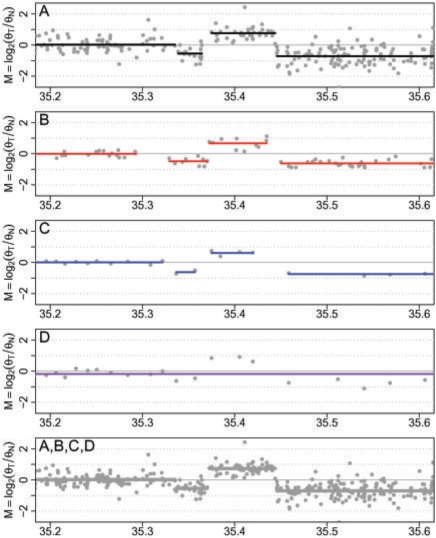
To further illustrate the effect of multisource normalization, we zoom in on a small part of the already studied 60 Mb region on Chr 3. In Figure 7, normalized CN estimates from the four sources as well as the combined normalized CNs are depicted for the 400 kb region at 35.2–35.6 Mb. It is clear that the different platforms have different densities overall, and also that their densities differ along the genome, i.e. the relative number of data points for Platform C (D) compared with Platform A, is much lower than the genome-wide average of 13% (Table 1). Note also that there exist regions where there are no observations available for some sources, e.g. around 35.3 Mb there are no CNs available from Source B, but several from Source A. This shows that integrating estimates from different platforms not only enhances the resolution, but increases the coverage, i.e. the platforms complement each other at different regions of the genome. Moreover, the fact that there are no data points for one of the platforms in certain regions is an argument for avoiding integrating CN data at the segmentation level, because it is often not clear from the results why a segmentation method identifies a CN aberration based on one platform but not based on another. It can either be because the aberration is false, or because the other platform has no data in that region. When integrating the data at the level of full-resolution CNs, this is less of a problem. The piecewise constant lines in Figure 7 show the CN regions as identified by the Circular-Binary Segmentation (CBS) method (Venkatraman and Olshen, 2007). We note that for this particular region, no aberrations are identified by the data from Source D. We believe that this is less likely to happen with with full-resolution normalized and combined CNs, and that there is more power to detect true CN regions. We also note that the precision of an estimated change point is greater when the density is greater, simply because the distance between any two loci is smaller.

Fig. 7.

Segmentation of a 400 kb region on Chr 3 using CN estimates from the individual sources (upper four panels) and the combined estimates (lower panel). In addition to increase density and effective resolution, the different sources also complement each other by covering different regions. All data are normalized across sources.

4 DISCUSSION

The proposed method controls for differences in mean levels between sources. It does not control for differences in noise levels. This implies that the variance of a normalized CN estimate in the combined dataset depends on the source of that CN estimate. In order for segmentation methods to perform optimally, this heteroscedacity needs to be taken into account. Segmentation methods, such as GLAD (Hupé et al., 2004) and CBS (Venkatraman and Olshen, 2007), which are most commonly used and well tested, do often not model heteroscedasticity of CNs, although they could be extended to do so. To the best of our knowledge, the only segmentation method readily available for doing this is the recently published HaarSeg method (Ben-Yaacov and Eldar, 2008). In the hidden Markov Model domain, there is the BioHMM method (Marioni et al., 2006). The performance of these methods is not known or not known as well as the aforementioned ones. Regardless, it is still possible to use ordinary segmentation methods, but their performance will be sub-optimal. The main difference is that by not controlling for heteroscedasticity, the CN estimates from the more noisy sources will have a relatively greater impact on the segmentation than if their greater variance would be accounted for.

It has recently come to our attention that one research group is developing a multitrack segmentation method for estimating segments common across sources, while taking heteroscedasticity and different mean levels into account. Their method assumes linear relationships between sources. When this is not true, as observed here, our method can normalize the data such that this assumption is met. We look forward to this new method.

Here, we have focused on CN estimates from different labs and technologies, but the proposed model and method may also be applied for normalizing estimates from different chip types of the same technology, e.g. when combining data from the two chip types part of the Affymetrix 500K chip set. Furthermore, the proposed normalization method makes it possible to combine data from different generations of arrays such as the Affymetrix 100K and the Affymetrix 6.0 chip types. This provides an alternative to existing methods for combining data across different generations of arrays (Kong et al., 2005). Similarly, the more recent chip types have markers for non-polymorphic loci in addition to markers for single-nucleotide polymorphism (SNP). If the assay or the preprocessing method produces CNs such that these two types of markers are not on the same scale, then our method may be used to normalize for differences in the SNP and non-polymorphic subsets.

Note that calibration and normalization functions may be estimated on a subset of existing loci. Hence, it is still possible to normalize data where one source completely lacks observations in parts of the genome. This also means that by using technologies complementing each other, including not only microarrays but also PCR and next-generation sequencing, an increased coverage in addition to an increased density can be obtained.

We further note that it is possible to normalize for differences between sources using quantile normalization (Bolstad et al., 2003). However, methods that normalize for differences in quantiles do not incorporate the genomic locations by coupling estimates from the same region across sources, cf. Equation (6). For a further discussion on relationships between normalization functions as defined here and quantile normalization, see (Bengtsson and Hössjer, 2006).

The MSCN method requires that for each sample there exists a few CN aberrations and other discrepancies from the copy neutral state in the genome. If not, the normalization functions are not identifiable. We do not know to what extent this could be a problem, especially in normal samples. The existence of CN polymorphic regions (CNVs) in normal individuals (Komura et al., 2006; Redon et al., 2006) should provide some protection against this. If not, Bayesian techniques where prior distributions of {h_s(·)} are obtained from other samples may be used. We look forward to further studies and reports on this.

REFERENCES

- Ben-Yaacov E, Eldar YC. A fast and flexible method for the segmentation of aCGH data. Bioinformatics. 2008;24:i139–i145. doi: 10.1093/bioinformatics/btn272. [DOI] [PubMed] [Google Scholar]
- Bengtsson H. Ph.D. Thesis, Centre for Mathematical Sciences, Division of Mathematical Statistics. Lund University; 2004. Low-level analysis of microarray data. [Google Scholar]
- Bengtsson H, Hössjer O. Methodological study of affine transformations of gene expression data with proposed robust non-parametric multi-dimensional normalization method. BMC Bioinformatics. 2006;7:100. doi: 10.1186/1471-2105-7-100. [DOI] [PMC free article] [PubMed] [Google Scholar]
- Bengtsson H, et al. Calibration and assessment of channel-specific biases in microarray data with extended dynamical range. BMC Bioinformatics. 2004;5:177. doi: 10.1186/1471-2105-5-177. [DOI] [PMC free article] [PubMed] [Google Scholar]
- Bengtsson H, et al. Technical Report 745. Berkeley: Department of Statistics, University of California; 2008a. aroma.affymetrix: a generic framework in R for analyzing small to very large Affymetrix data sets in bounded memory. [Google Scholar]
- Bengtsson H, et al. Estimation and assessment of raw copy numbers at the single locus level. Bioinformatics. 2008b;24:759–767. doi: 10.1093/bioinformatics/btn016. [DOI] [PubMed] [Google Scholar]
- Bolstad B, et al. A comparison of normalization methods for high density oligonucleotide array data based on variance and bias. Bioinformatics. 2003;19:185–193. doi: 10.1093/bioinformatics/19.2.185. [DOI] [PubMed] [Google Scholar]
- Collins FS, Barker AD. Mapping the cancer genome. Sci. Am. 2007;296:50–57. [PubMed] [Google Scholar]
- Hastie T, Stuetzle W. Principal curves. J. Am. Stat. Assoc. 1989;84:502–516. [Google Scholar]
- Hupé P, et al. Analysis of array CGH data: from signal ratio to gain and loss of DNA regions. Bioinformatics. 2004;20:3413–3422. doi: 10.1093/bioinformatics/bth418. [DOI] [PubMed] [Google Scholar]
- Komura D, et al. Genome-wide detection of human copy number variations using high-density DNA oligonucleotide arrays. Genome Res. 2006;16:1575–1584. doi: 10.1101/gr.5629106. [DOI] [PMC free article] [PubMed] [Google Scholar]
- Kong SW, et al. CrossChip: a system supporting comparative analysis of different generations of Affymetrix arrays. Bioinformatics. 2005;21:2116–2117. doi: 10.1093/bioinformatics/bti288. [DOI] [PMC free article] [PubMed] [Google Scholar]
- Korn JM, et al. Integrated genotype calling and association analysis of SNPs, common copy number polymorphisms and rare CNVs. Nat. Genet. 2008;40:1253–1260. doi: 10.1038/ng.237. [DOI] [PMC free article] [PubMed] [Google Scholar]
- Marioni JC, et al. BioHMM: a heterogeneous hidden Markov model for segmenting array CGH data. Bioinformatics. 2006;22:1144–1146. doi: 10.1093/bioinformatics/btl089. [DOI] [PubMed] [Google Scholar]
- TCGA Network,C.G.A.R. Comprehensive genomic characterization defines human glioblastoma genes and core pathways. Nature. 2008;455:1061–1068. doi: 10.1038/nature07385. [DOI] [PMC free article] [PubMed] [Google Scholar]
- Page ES. A test for a change in a parameter occurring at an unknown point. Biometrika. 1955;42:523–527. [Google Scholar]
- R Development Core Team. R: A Language and Environment for Statistical Computing. R Foundation for Statistical Computing, Vienna, Austria. 2008. ISBN 3-900051-07-0. [Google Scholar]
- Ramdas L, et al. Sources of nonlinearity in cDNA microarray expression measurements. Genome Biol. 2001;2 doi: 10.1186/gb-2001-2-11-research0047. research0047.1–0047.7. [DOI] [PMC free article] [PubMed] [Google Scholar]
- Redon R, et al. Global variation in copy number in the human genome. Nature. 2006;444:444–454. doi: 10.1038/nature05329. [DOI] [PMC free article] [PubMed] [Google Scholar]
- Venkatraman ES, Olshen AB. A faster circular binary segmentation algorithm for the analysis of array CGH data. Bioinformatics. 2007;23:657–663. doi: 10.1093/bioinformatics/btl646. [DOI] [PubMed] [Google Scholar]
- von Neumann J, et al. The mean square successive difference. Ann. Math. Stat. 1941;12:153–162. [Google Scholar]
- Weingessel A, Hastie T. princurve: Fits a Principal Curve in Arbitrary Dimension. 2007 [Google Scholar]
- Ylstra B, et al. BAC to the future! or oligonucleotides: a perspective for micro array comparative genomic hybridization (array CGH) Nucleic Acids Res. 2006;34:445–450. doi: 10.1093/nar/gkj456. [DOI] [PMC free article] [PubMed] [Google Scholar]