Differential quantitative proteomics of Porphyromonas gingivalis by linear ion trap mass spectrometry: non-label methods comparison, q-values and LOWESS curve fitting

Abstract

Differential analysis of whole cell proteomes by mass spectrometry has largely been applied using various forms of stable isotope labeling. While metabolic stable isotope labeling has been the method of choice, it is often not possible to apply such an approach. Four different label free ways of calculating expression ratios in a classic “two-state” experiment are compared: signal intensity at the peptide level, signal intensity at the protein level, spectral counting at the peptide level, and spectral counting at the protein level. The quantitative data were mined from a dataset of 1245 qualitatively identified proteins, about 56% of the protein encoding open reading frames from Porphyromonas gingivalis, a Gram-negative intracellular pathogen being studied under extracellular and intracellular conditions. Two different control populations were compared against P. gingivalis internalized within a model human target cell line. The q-value statistic, a measure of false discovery rate previously applied to transcription microarrays, was applied to proteomics data. For spectral counting, the most logically consistent estimate of random error came from applying the locally weighted scatter plot smoothing procedure (LOWESS) to the most extreme ratios generated from a control technical replicate, thus setting upper and lower bounds for the region of experimentally observed random error.

1. Introduction

Tandem mass spectrometry coupled with multiple dimensions of HPLC has evolved in recent years to become a standard approach to genome-wide analysis of whole cell protein mixtures. Differential protein expression analysis of whole cell proteomes by mass spectrometry has largely been accomplished using stable isotope labeling methods [1]. However, isotope labeling inevitably increases sample complexity and decreases qualitative proteome coverage, partly due to the duty cycle limits of current mass spectrometry technology and the need to collect data simultaneously for both the labeled and unlabeled peptides sharing the same amino acid sequence.

In this paper, we examine four different ways of calculating relative protein expression ratios, derived from linear ion trap data, in the absence of stable isotope labeling. Two of the approaches involve a continuous variable, signal intensity, and two involve a discrete (discontinuous) variable, the number of peptide mass spectra observed, referred to here as spectral counts. These two types of data can both potentially address the primary question of interest in such studies: does a given protein change expression level between two biologically distinct states, or does it stay the same?

Spectral counting has been proposed as a method for quantitative proteomics by mass spectrometry [2-6]. Liu, Sadygov and Yates [3] demonstrated a linear relationship between sampling level, that is the number of peptide mass spectra observed, and the relative abundance of a protein in a complex. Old and coworkers [4] have recently performed comparative studies of non-label quantitative methods using well-characterized reference proteins and human erythroleukemia K562 cells. Here we apply two variations on the theme of spectral counting to large-scale proteomic datasets from studies of the interaction of a well-known oral pathogen with a model human host cell system. One approach is the way common to the references cited above, that is to count the observed mass spectra for each proteolytic fragment from a given protein and use that number as a measure of protein relative abundance and as one input into a relative expression calculation. This will be referred to as the protein level spectral counting method. The other approach is to treat each unique peptide as a group instead of each protein. A unique peptide is defined here as a proteolytic fragment that maps to only one expressed protein for the organism under investigation. All unique peptides for each protein are then grouped and the expression ratio is calculated by averaging the ratios from the peptides. This will be referred to as the peptide level spectral counting method. The peptide level spectral counting method was felt to have potential advantages, such as more data points collected for each protein. The signal intensity methods use the sum of MS¹ signal intensity as an indicator for relative abundance. By analogy with the definitions given above, the signal intensity approach can be applied at the level of unique peptides or at the reconstructed protein level. These methods will be referred to as peptide level signal intensity and protein level signal intensity, respectively. It was our initial hypothesis that for high signal-to-noise data indicative of a biologically significant change in protein expression for a given ORF, all four methods would agree in terms of the direction of change, but not in the magnitude of change. Initially, we did not expect any single approach to be greatly superior to the others. All were expected to be inferior to metabolic labeling in terms of quantitative coverage of the proteome, based on studies of another prokaryote with a similar number of protein encoding ORFs. For Methanococcus maripaludis, a methanogenic Archaeon, quantitative proteome coverage was approximately 50% better using ¹⁵N/¹⁴N ratios when compared to processing the same raw data using protein level spectral counting as defined above [7].

P. gingivalis is a highly invasive intracellular oral pathogenic bacteria involved in adult periodontitis [8]. The W83 strain genome has been sequenced and the completed genome sequence information was added to the Comprehensive Microbial Resource of TIGR on June 8, 2001 [9]. In previous studies, we used conditioned keratinocyte growth medium (cKGM) to simulate the early stages of P. gingivalis invasion of human gingival epithelial cells [10]; cKGM is KGM enriched with the supernatant materials left after human gingival epithelial cell culturing. Recently, human immortalized gingival keratinocytes (HIGK) [11] have replaced primary human gingival epithelial cells for these studies. Differential protein expression analyses were performed to investigate the effects of internalization within HIGK on P. gingivalis protein expression. Because of technical problems encountered while growing ¹⁵N labeled P. gingivalis on minimal media with ¹⁵N ammonium sulfate as the only nitrogen source, we have studied alternative non-label approaches to generating protein expression ratios in which two control populations of P. gingivalis are compared to a population of bacteria that has been internalized within HIGK. The experimental design thus consisted of three populations of P. gingivalis cells analyzed using four quantitative methods, as shown in Table 1. The focus in this report is analytical and methodological. A biologically based discussion of the quantitative changes observed in the P. gingivalis proteome will appear in a future publication.

Table 1.

Experimental design for two internalized bacteria/control comparisons and four methods for calculating protein expression ratios. The variable ScRatio1 thus represents the ratio of internalized PG and PG controls grown under normal culture conditions (see 2.1) calculated using the protein level spectral count method. The other seven conditions are defined analogously according to their position in the table.

	PG_PP/PG_nm		PG_PP/PG_PPC
	Protein level	Peptide level	Protein level	Peptide level
Spectral count	ScRatio1	ScRatio3	ScRatio2	ScRatio4
Signal intensity	PiRatio1	PiRatio3	PiRatio2	PiRatio4

2. Materials and methods

2.1. Sample preparation, HPLC fractionation and tandem mass spectrometry

There were three samples of P. gingivalis strain 33277: P. gingivalis cells cultivated to mid-log phase in trypticase soy broth supplemented with yeast extract (1 mg ml^-1), menadione (1 μg ml^-1) and hemin (5 μg ml^-1), at 37°C under anaerobic conditions of 85% N₂, 10% H₂ and 5% CO₂, referred to as PG_nm or PG normal; P. gingivalis cells incubated in fresh HIGK cell culture medium (Keratinocyte-SFM from GIBCO, Invitrogen Corporation, catalogue number 17005) for 18 h anaerobically at 37°C, referred to as PG_PPC; and P. gingivalis cells recovered after an 18 hour period of internalization within HIGK cells and lysis of the HIGK cells with distilled water, referred to as PG_PP. P. gingivalis cells were washed once with distilled water and recovered by centrifugation. Cell pellets containing approximately 10⁹ cells were resuspended with 100 μl 0.1 M Tris buffer (pH 8.0), 50 μl RapiGest (1mg/100 μl) in a 1.5 ml microcentrifuge tube. Four μl of 1M DTT and 30 μl DNAse/RNAse solution (1 mg/ml DNAse I, 500 μg/ml RNAse A, 50 mM MgCl₂, 50 mM Tris-HCl at pH 7.0) was added into the suspension. The samples were immediately placed in 100 μl of boiling 0.1 M Tris buffer (pH 8.0) for 5 min until the solution ceased to show obvious viscosity due to residual DNA. Each sample was then transferred onto ice. The proteins were further reduced by the addition of 5 mM DTT at 37°C for 30 min and then alkylated with 30 mM iodoacetamide at 30°C for 30 min in the dark. Each sample was then adjusted to give a solution containing 50 mM Tris, pH 8.0 and 5 mM CaCl₂. Trypsin, 10 μg of sequencing grade (Promega, Madison, WI), was added, and the mixture was incubated at 37°C for 4 hours. The samples were centrifuged at 14,000 rpm for 7 min. The supernatant was transferred to another 1.5 ml microcentrifuge tube. The insoluble fraction was kept at −80°C for further analysis. The samples were acidified with TFA to quench the digestion and concentrated to 200 μl using a vacuum centrifuge (RC10-22, Jouan Inc. Winchester, VA). The supernatant from the digestion step described above was thawed and centrifuged at 14,000 rpm for 6 min. The solution was loaded onto a 2.0 × 150 mm YMC polymer C18 S-6 reversed-phase HPLC column (Waters Corp., Milford, MA, USA). The mobile phases were H₂O and acetonitrile with 0.1% TFA. Peptides were eluted with increasing acetonitrile percentage (2%-50% for 50 min, 50% - 2% in 5 min.) at 0.3 ml/min. Eluent was collected into five fractions according to UV absorption at 214 nm. Each fraction was concentrated to 50 μl using the vacuum microcentrifuge. Acetic acid and acetonitrile were added to a final concentration of 0.5% and 5% (v/v), respectively.

The insoluble fraction was dissolved in 50 μl of 8M urea and 0.125% (w/v) RapiGest. The proteins were reduced with 5 mM DTT at 37°C for 30 min and then alkylated with 10 mM iodoacetamide at 30°C for 30 min in the dark. After addition of 100 μl of 0.1M Tris (pH 8.0), CaCl₂ and acetonitrile were added, 5mM and 5% respectively. 10 μg of trypsin (sequencing grade, Promega, Madison, WI, USA) was added and the mixture was incubated at 37°C for 4 hr. Five μl of TFA was added to the mixture to stop the digestion. RapiGest was degraded and precipitated by incubating at 37°C for 30 min. The solution was centrifuged at 14,000 rpm for 6 min. The precipitate was washed twice with 40 ul of 50 mM Tris pH 8.0. The soluble fraction and combined washes were desalted and fractionated as described above except that peptides were eluted with a gradient of 2%-70% acetonitrile for 50 min. Eluent was collected into one fraction for PG_nm (P. gingivalis in normal growth medium) and PG_PPC (P. gingivalis in control epithelial cell culture medium), and two fractions for PG_PP (P. gingivalis recovered from inside epithelial cells), based on the more intense UV absorbance (214 nm) observed for PG_PP. Fractions of PG_nm and PG_PPC were concentrated to 25 μl using the vacuum microcentrifuge. Fractions of PG_PP were concentrated to 50 μl. Acetic acid and acetonitrile were added to a final concentration of 0.5% and 5% (v/v) respectively. Approximately 2.5 μl from each combined fraction was analyzed using a 2D microcapillary HPLC system [10, 12] combined with a Thermo-Finnigan LTQ mass spectrometer in a semi-automated, data-dependent manner as previously described [13]. Peptides were first partially eluted from the SCX (strong cation exchange) packing, and were retained on the reverse phase material by ammonium acetate step gradients (0, 10, 25, 50, 100, 250, 500 mM). The peptides were eluted from the reverse phase packing with an acetonitrile gradient with 0.5% v/v acetic acid, and were electrosprayed into the LTQ for data-dependent acquisition. The gradients programmed were: 5% B, hold 13 min, 5–16% B in 1 min, hold 6 min, 16–45% B in 45 min, 45-80% B in 1 min, hold 9 min, 80-5% in 5 min, hold 10 min. The flow rate in the capillary column was 150 nl/min during 16-45% B and 300 nl/min during all other gradient sections. The MS¹ scan range was 400–2000 m/z units acquired at a rate of 16,600 u/sec. After each main beam (MS¹) scan, the ten most intense m/z values above 20,000 counts were selected for collision-induced dissociation (CID, MS²), each complete cycle of MS¹ and MS² taking between 3.0 and 3.6 sec. Default parameters under the Xcalibur 1.4 data acquisition software (Thermo Finnigan, San Jose, CA, USA) were used, with the exception of an isolation width of 3.0 m/z units. Automatic gain control and dynamic exclusion (30 sec window, 10 ions) were activated during all acquisitions.

2.2 Database searching and DTASelect

MS/MS spectra were searched by SEQUEST [14] on a 16-CPU cluster computer (Denali Advanced Integration, USA) against a combined fasta database which includes the temporary bovine database from the University of California at Santa Cruz [15], bovine fasta database from the nrdb of the National Center for Biotechnology Information [16], human fasta database from the nrdb [16], NIH Mammalian Gene Collection [17, 18] and the P. gingivalis database from TIGR [9]. DTASelect [19] filtering was done by applying the following criteria: peptides were fully tryptic (beginning and ending at adjacent predicted trypsin digestion sites); ΔCn/Xcorr values for different peptide charge states were 0.08/1.9 for +1, 0.08/2.0 for + 2, and 0.08/3.3 for +3; all spectra detected for each sequence were retained (t = 0 in DTASelect).

2.3 Data processing for relative quantitation

The data processing steps for relative quantitation were as follows: first, the raw files were converted to text files by the file converter in the Xcalibur 1.4 data system for the LTQ. Then, a Visual Basic for Applications program was run in Microsoft Word to extract the full scan number, ion m/z value and intensity from the text file. A relational database was constructed in FileMaker Pro 8. The DTASelect-filter file and each intensity file was imported into FileMaker Pro 8 as separate tables. Identical multiple criteria relationships between each intensity table and the DTASelect-filter table were established by the following rules: the m/z value in the DTASelect-filter file was kept within the m/z range of the intensity file plus or minus the m/z tolerance (we use ± 0.2); and the full scan value in the DTASelect-filter file was within the range of the full scan number in the intensity file plus or minus the full scan number tolerance (± 30 scans). Then, a FileMaker script was used to update the intensity and full scan fields in the DTASelect-filter table. Because the DTASelect-filter to intensity file relationships were defined to always sort the intensity files in descending order of signal intensity, the updated intensity field in the DTASelect-filter table was the value from the highest mass peak for the corresponding CID parent ion among the ± 30 scans.

2.4 Four relative quantitation methods for generating expression ratios

Calculating the protein level spectral count was straightforward. In the DTASelect-filter file, the number of each SEQUEST identified spectra was listed with each ORF. That number was used as the protein level spectral count. The ratio of each protein from two samples (PG_PP/PG_nm or PG_PP/PG_PPC, see Table 1) was then calculated from the two spectral count values after the normalization steps described below.

For the peptide level spectral counting method, the spectral count of each peptide was calculated by averaging the spectral counts from two technical replicates. For those identified in only one replicate, that number was used as the spectral count. Then, after normalization, for each peptide the ratio of two samples (PG_PP/PG_nm or PG_PP/PG_PPC) was calculated. In the case when the peptide was only detected in one sample, 1 was added to the peptide level spectral count in order to avoid a count of zero. The protein level peptide intensity method used all the intensity values from all peptides identified for one protein, including redundant measurements. The sum of the intensity values in MS¹ was used to represent the abundance of each protein in the sample. For the peptide level peptide intensity method, the summed intensity in MS¹ for each unique peptide sequence was calculated by adding the signal intensity within each technical replicate, then averaging the totals for the technical replicates. For those peptides identified in only one replicate, the summed intensity was used. Then, for each unique peptide, after normalization, the ratio of two samples (PG_PP/PG_nm or PG_PP/PG_PPC) was calculated from the average summed intensity values. In the case when peptide was only detected in one sample, 20,000 counts of processed signal intensity was added to the peptide as its summed intensity in order to avoid generating missing ratios. This number of counts corresponded to the average baseline threshold for selecting CID ions in MS¹.

2.5 Normalization of spectral counts and peptide intensities prior to calculating ratios

PG_PP/PG_nm spectral count ratios (both peptide level and protein level) were normalized by multiplying PG_PP spectral counts by a factor of 2.43 to make the sum of spectral counts in PG_PP and PG_nm equal; PG_PP/PG_PPC spectral count ratios were normalized by multiplying PG_PP spectral counts by 1.68; PG_PP/PG_nm peptide intensity ratios were normalized by multiplying PG_PP peptide intensities by 3.31 to make the sum of peptide intensities in PG_PP and PG_nm equal; PG_PP/PG_PPC peptide intensity ratios were normalized by multiplying PG_PP peptide intensities by 1.75.

2.6 Outlier detection for expression ratios

Detection of outliers for normalized ratios generated for the peptide level spectral count and peptide level peptide intensity methods was done in two steps for each list of ratios associated with an ORF, as we have published for metabolic labeling data [13]. For the first stage, Dixon's Q-test [20] was used, in the second stage, a MAD (median of the absolute deviation) modified z-score test [21-23] with a cutoff value of 3.5 was used.

2.7 Statistical significance testing and curve fitting

The G statistic, two sample t-test, p-value, and q-value calculations were calculated using the R language [24]. R code was modified in-house from source code kindly provided by the Department of Statistics Consulting Service of the University of Washington. The relevant theory is given in the following section. The LOWESS (locally weighted scatter plot smoothing) curve fitting [25] shown in Fig. 1 was performed using R code developed in-house. The R source code is provided in the Electronic Supplement.

Fig. 1.

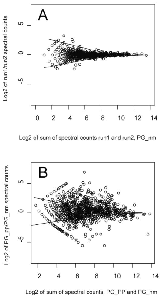
A. Scatter plot of log₂ of run1/run2 spectral count ratios versus log₂ of protein level spectral counts from run1 and run2 of PG_nm. B. Log₂ of PG_PP/PG_nm spectral count ratios versus log₂ summed protein level spectral counts from PG_PP/PG_nm. The two solid curves shown are the LOWESS smoothing curves [25] of the upper and lower boundary of the log₂ ratios of protein level spectral counts from the control replicates, PG_nm.

3. Theory and calculations

3.1 G test for protein level spectral counting

The G test of significance [26] we chose for protein level spectral counting is a likelihood ratio test for discrete data, which was recently applied to human proteomics data by Old and coworkers in their study of non-label quantitation [4]. For the PG_PP and PG_nm comparison, we first normalized the PG_PP spectral counts with PG_nm by transforming the spectral counts of each protein in PG_PP so that the sums of spectral counts in PG_PP and PG_nm were the same, based on the assumption that the PG_PP and PG_nm frequency distributions were similar and from samples of the same size. We then set the expected frequency, also known as the expectation value, equal to the average frequency of the two samples. That is, set

$${\hat{f}}_{PP}={\hat{f}}_{NM}=\frac{f_{PP}+f_{NM}}{2}$$ (1)

where f_PP and f_NM are spectral counts for a given protein in PG_PP and PG_nm; f̂_PP and f̂_NM are expected protein level spectral counts in PG_PP and PG_nm under the null hypothesis that there is no difference in expression of the protein between PG_PP and PG_nm.

Our G-statistic then becomes

$$G=2\left[f_{NM}·ln\left(\frac{f_{NM}}{\frac{f_{NM}+f_{PP}}{2}}\right)+f_{PP}·ln\left(\frac{f_{PP}}{\frac{f_{NM}+f_{PP}}{2}}\right)\right]$$ (2)

A G statistic used in this way is expected to approximate a χ² distribution with 1 degree of freedom [26]. In order to verify this assumption for a χ² distribution with 1 degree of freedom, G test simulations with frequencies from two binomial distributions with equal sample sizes (n) and proportions (p) were carried out. Details are presented in the Appendix and the R code contained in the Electronic Supplement. The simulated distribution did not match the χ² distribution, except at the lowest proportion values, see Appendix Fig. A1. However, this simulation did indicate that p-values calculated using this assumption should be conservative. In other words, fewer proteins were likely to be judged significantly over- or under-expressed in the internalized population relative to the controls and the false positive risk would be reduced at the expense of increasing the risk of false negatives.

Fig. A1.

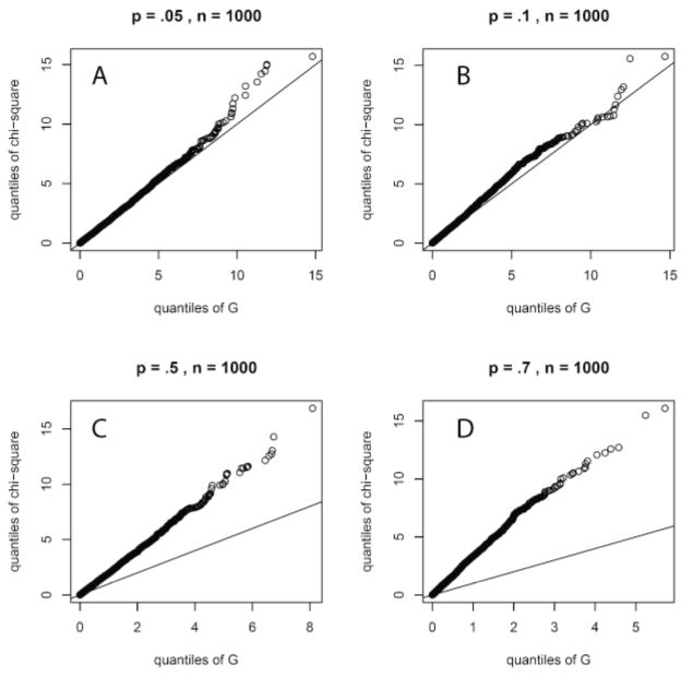
Quantile-quantile (q-q) plots of Chi-square versus G statistic at four levels of proportion value. The assumption of equivalence is violated to a greater degree as the proportion value increases.

3.2 q-value calculations

Controlling for false positives has been proposed using a q-value rather than a p-value. The q-value is closely related to the concept of false discovery rate, FDR, and has been defined as a measure of the strength of an observed statistic, in this case a p-value, with respect to the positive false discovery rate, pFDR [27]. In the context of this paper, it is the minimum pFDR that can occur when rejecting the null hypothesis (no change in protein expression) at a certain p-value. After generating a G-test statistic for each protein, a p-value was calculated as the probability that a χ² distribution with 1 degree of freedom was more extreme than our G statistic. The R package QVALUE [27, 28] was used to calculate q-values for each protein based on the p-value.

3.3 Two sample t-test

For the protein level peptide intensity method, a two-sample t-test was performed for each protein. The two-sample t-statistic was

$$t=\frac{X-Y}{\sqrt{m\cdot s_x^2+n\cdot s_Y^2}}$$ (3)

where X and Y are the sum of peptide signal intensities from the two conditions being compared; s_x and s_y are the standard deviations, and n and m are the number of peptide spectra observed for the protein under each condition. The p-values were then calculated as the probability that a standard normal distribution was more extreme than our two-sample t-statistic. The R package QVALUE [27, 28] was used to calculate q-values for each protein based on the p-value.

4. Results and discussion

4.1 Proteome qualitative coverage

From this study, 1245 total P. gingivalis proteins were qualitatively identified in Pg_nm, PG_PPC and PG_PP. 1137 proteins were identified in PG_nm, 987 proteins in PG_PP and 1068 proteins in PG_PPC. According to TIGR [9], the P. gingivalis W83 database contains about 2,227 protein encoding ORFs, and the 33277 strain used here is believed to be very similar. These facts suggest proteome coverage of ∼56% of the predicted ORFs.

4.2 Correlations among the four calculation methods

As can be seen from an inspection of the representative scatter plots and correlation coefficients shown in Fig. 2, the four methods gave results that were strongly correlated, as expected. The best correlations were observed between the two spectral counting methods, the worst between the peptide intensity methods. This is consistent with the observation that spectral counting data tends to be less noisy and more reproducible relative to intensity-based methods, although such a statement must be subject to several caveats. Most important among these is the generally poor performance of spectral counting approaches when peptide numbers are low, as evidenced by the wide scatter for low peptide numbers shown in Fig. 1.

Fig. 2.

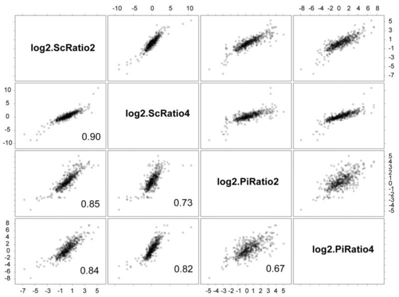
Scatter plot matrix generated in S-PLUS 6.0 (www.insightful.com) showing correlation coefficients for the four methods. The scatter plots were generated from 528 data points for the PG_PP/PG_PPC expression ratios. See Table 1 and the Introduction for definitions of the variables.

The Venn diagrams in Fig. 3 show the overlapping subsets of ratios calculated by the four methods for the two controls that were each compared with internalized bacteria (see Table 1). From the Venn diagrams, for PG_PP/PG_nm, 37 up-regulated and 18 down-regulated ORFs were reported by all methods; 185 up-regulated and 137 down-regulated ORFs were reported by at least three out of the four methods. Moreover, for PG_PP/PG_PPC, 35 were up-regulated and eight down-regulated by all methods; 146 were up-regulated and 126 were down-regulated by at least three out of the four methods. If we choose significant expression changes reported by at least three out of the four methods as criteria, we have 322 ORFs in PG_PP/PG_nm and 272 ORFs in PG_PP/PG_PPC. These numbers are closer to estimates suggested by biological arguments [10, 29] and also the numbers suggested by the interpretation of Fig. 1 given in Section 4.4 below. The similarities and differences among the different calculation methods with respect to defining the expression status of each ORF can be inspected visually by viewing the eight whole proteome false color ORF plots contained in the Electronic Supplement, Figs. S1-S8.

Fig. 3.

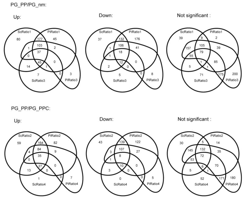
Standard four-statement Venn diagrams showing the overlap of detected significant and non-significant expression changes among the four different non-labeling quantitation methods (see Table 1 for definitions). The criteria for determining significance was the following: for protein level ratios, the q-value was less than 0.05; for peptide level ratios, the log₂ ratio − SD was > 0 or the log₂ ratio + SD was < 0.

There were 20 ORFs contained in the most restricted subset of significant expression changes, defined by changes in the same direction in both comparisons and by all calculation methods. A somewhat restricted overlap among all four methods and both controls was not unexpected, given the highly conservative selection criteria. The data for these 20 ORFs are given in the Electronic Supplement, Tables S1 and S2.

4.3 Repeatability of spectral counting data

Fig. 4 shows the correlation of spectral counts for each protein identified from three replicate runs of PG_PP. As shown in the three panels, the spectral counts for each of the 751 commonly identified proteins in all three runs demonstrate a very consistent linear relationship. In other words, the spectral count of one protein in a complex sample consisting of many tens of thousands of proteolytic fragments is a surprisingly stable measurement under these experimental conditions.

Fig. 4.

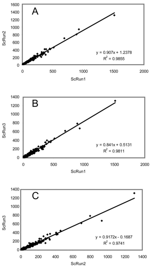
Scatter plots on a linear scale and correlation statistics for spectral counts from three technical replicates of PG_PP, showing repeatability of the spectral count method. Each data point represents the number of peptide MS¹ spectra retained for each protein. These plots were generated in S-PLUS 6.0 (www.insightful.com) for proteins commonly identified in all three runs.

4.4 Visualizing random errors in spectral counting

When the sum of spectral counts of technical replicate runs is less than roughly 10, the ratios calculated are too noisy and quantized to be of further use (Fig. 1A). For the peptide level spectral count method, we did not use any peptide whose sum of spectral counts for any two samples or replicates was less than 10. When the sum of spectral counts goes to large values, the log₂-transformed ratios tend towards zero except in the case of a real difference between the two data sets being compared. Outliers due to experimental error are infrequent at high counts. For purposes of comparison, Fig. 1B shows a much more scattered relationship between the ratios of PG_PP/PG_nm and the sum of spectral counts, which supports an increasing body of observations suggesting that there are hundreds of P. gingivalis genes showing altered expression in PG_PP relative to controls [10, 29-31]. The data shown in Fig. 1 suggests that it should be possible to use the error distribution of the expression ratios observed for replicate runs of the same sample (Fig. 1A) to distinguish true expression changes from random errors when comparing two different samples (Fig. 1B). This concept could easily be extended to biological replicates as well. The LOWESS smoothing curves [25] of the upper and lower boundaries in Fig. 1A essentially demarcate the region of observed experimental error that can be attributed to instrumental causes. It is reasonable to interpret expression ratios that fall within this region as random error. Such curve fitting approaches have been successfully applied to visualizing regions of random error in transcription microarray data [32, 33]. Those same boundaries are shown superimposed on a real experiment comparing internalized bacteria and a control population in Fig. 1B. In Fig. 5, the overlap of the significant results falling outside the boundary of the LOWESS lines is compared with a q-value cutoff of 0.05. All values judged to be significant based on the LOWESS curve fit were contained in the set at q = 0.05, but an additional 113 ratios gave q ≤ 0.05. Thus, the curve fit by itself yielded a numerically smaller estimate of the number of proteins showing a significant change in expression. Whatever the true nature of the ratios that fall outside the boundaries defined by the LOWESS curve, the procedure allows the analyst to quickly visualize those ratios that are worth examining in greater detail, and also the vast majority that fall within the region bounded by the curve where, from an experimental perspective, true expression change cannot be distinguished from random error.

Fig. 5.

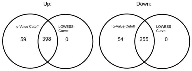
Venn diagrams showing the comparison of the significant changes of PG_PP versus PG_nm from the protein level spectral count (ScRatio1) method with q = 0.05 and the significant proteins that are outside the LOWESS curves in Fig. 1B. For both up and down expression changes, the proteins that were outside the LOWESS curves in Fig. 1B were all included in the ScRatio1 results.

4.5 Assumptions violated when many proteins change

The assumptions behind our G test statistic, Eq. (2), were almost certainly violated to such a degree that the results, based purely on theoretical considerations, should have been biased in a conservative direction, given that the expectation values were based on expression ratios from a proteome believed to be highly regulated (see 4.4). If a large number of ratios are derived from highly regulated proteins, the expectation values defined by Eq. (1) are going to be skewed towards the direction of treating biologically significant changes as null. The normalization methods commonly used for transcription microarrays [34] and for shotgun proteomics also make assumptions that only a few genes or proteins among many are changing. These are reasons why the experimentally observed error distribution (Fig. 1) and the simple graphical method discussed above in 4.4 are of practical interest as checks on both our multiple hypothesis testing procedures and data normalization.

4.6 Setting the q-value threshold for ratios calculated by protein level spectral counting and protein level signal intensity

Referring to Storey and Tibshirani [27], we generated a series of q-value frequency histograms as shown in Fig. 6. The flat region is interpreted as one where there is no significant change in expression. It was decided to take 0.05 as the q-value threshold. This value is represented by the dotted lines in Fig. 6. According to Storey [27], “the p-value is a measure of significance in terms of the false positive rate”, whereas “the q-value is a measure in terms of the false discovery rate”. Therefore, when we take 0.05 as the q-value threshold, among all expression ratios called significant, 5% of them are predicted to be null on average. Alternatively, the LOWESS procedure described above in 4.4 can be used as an aid for establishing a reasonable value for the q-value cutoff, analogously to the procedure shown in Fig. 6. Interestingly, in spite of the problems noted above in 4.5 for the G test, the simple curve fit suggested an even smaller subset of potentially regulated proteins when compared to the subset with q ≤ 0.05, see Fig. 5. Further study will be required to fine tune our use of q-values to address concerns that 113 proteins deemed significant at q ≤ 0.05 fell within the bounds of random error determined experimentally (Fig. 1).

Fig. 6.

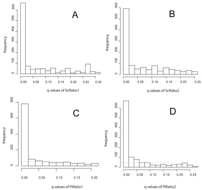
Frequency histograms of the q-values from ScRatio1 (A), ScRatio2 (B), PiRatio1(C) and PiRatio2 (D), see Table 1 for definitions. The dashed lines are at the height of our estimate of the proportion of null q-values. The y-axis represents the number of ORFs in each bin. The x-axis represents the q-values calculated as described in Sections 3.2 and 3.3.

4.7 Standard deviations are high for peptide level methods

Standard deviations for the peptide level methods were high because there are large variations in molar response and recovery among different peptides, regardless of their origin as part of a particular protein. As shown for a representative case in Fig. 7, the 26 peptides identified for major fimbrillin A (P13793|FMA_PORGI) demonstrate how great the variation of spectral counts and peptide signal intensity can be. Even for this very abundant protein, some peptides are identified with one or two CID spectra, while other peptides are identified with several thousand. Moreover, the range of peptide ion signal intensities can extend well beyond the dynamic range of the measurement process.

Fig. 7.

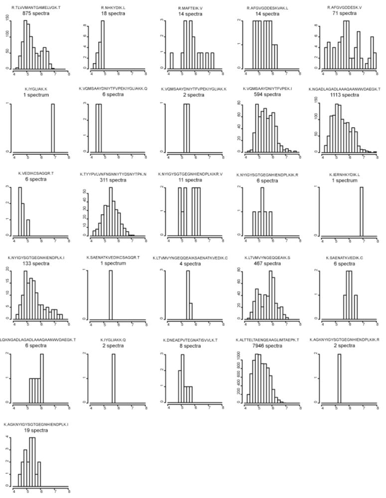
Frequency histograms of 26 identified peptides of P13793|FMA_PORGI, major fimbrillin A observed in sample PG_nm. The large variations in spectral counts and intensity distributions between different peptides can explain why the relative standard deviations of peptide level methods are so high. The y-axis of each histogram represents the number of peptide spectra in each bin. The x-axis represents signal intensity in units of log₁₀ data system counts.

5. Conclusions

The relationship of true protein abundance to spectral counting and peptide signal intensities from mass spectrometry data remains a topic of active investigation with few definitive answers and substantial disagreement as to how much coverage is required to generate biologically useful protein expression ratios. For example, Silva and coworkers [35] observed “the average MS signal response for the three most intense tryptic peptides per mol of protein is constant within a coefficient of variation of less than ± 10%.” Our data tend to support this observation. This trend can be seen for a representative protein in Fig. 7, where the top four peptides ranked in number of identified spectra show a much narrower range of values compared to the other 22 peptides. The methods defined in the Introduction as peptide level spectral counting and peptide level signal intensity both performed poorly (see 4.2) relative to the protein level methods, in terms of quantitative proteome coverage. While matching “heavy” and “light” peptides sharing the same sequence works well in a classic stable isotope quantitation scheme [36], where the peptides are analyzed at the same time, the random scatter in the data inevitably increases when an analogous approach is applied to unlabeled peptides sharing the same sequence but analyzed separately at different times. Thus, the error bars associated with ratios generated from our peptide level data were too large in many cases to distinguish the ratios from 1 on a linear scale or 0 on a log₂ scale, whether any expression change was occurring or not (see 4.2 -4.4). This can be seen graphically in the Venn diagrams (Fig. 3) in which the peptide level methods have significantly fewer ORFs in the up or down categories. Peptide level spectral counting yielded the fewest ORFs in the up or down category, the protein level methods the most, and the peptide level signal intensity approach fell between these extremes in terms of ability to detect expression change. The poor performance of the peptide level spectral counting approach in particular can be easily grasped by examining whole proteome color figures contained in the Electronic Supplement, that summarize the entire dataset for each set of conditions (Figs S1-S8).

To answer the question posited in the Introduction, of the methods we have tested the best approach to measuring protein expression changes in a bacterial cell, in the absence of stable isotope metabolic labeling, appears to be protein level spectral counting because of its better precision (see 4.2, 4.3, 4.7) relative to methods based on signal intensity or peptide level spectral counting.

The LOWESS curve fit to the technical replicates (Fig. 1, Section 4.4) shows promise as an easily implemented and logical way to visualize the random errors in determining expression ratios based on protein level spectral counting. It is also worthy of further study as a method for assessing the proper significance level of q-value that best fits the data in a more formal assessment of ORFs that show significant changes in expression level. Those ratios that appear to represent real, biologically significant expression can then be viewed as candidates for further validation. Using mass spectrometry, this can take the form of more specific post-acquisition data mining targeted at particular proteins of interest, or carrying out new experiments targeted at particular proteins, protein complexes, or posttranslational modifications, as discussed in a recent review of mass spectrometry applications in biomarker and drug discovery [37]. The question of biologically significant expression level change ultimately must be dealt with by using an approach in which other methods are brought to bare on the problem, e.g. the use of transcription microarrays, quantitative RT-PCR, functional assays and other means as required. A whole cell shotgun proteomics experiment, no matter how well executed, requires validation by an orthogonal approach. An elegant example of proteomics applied in such a systems biology context can be found in the recent study by Becker et al. [38] of potential targets for antibacterial drugs in the Salmonella enterica proteome.

Abbreviations

FDR

false discovery rate

HPLC

high performance liquid chromatography

HIGK

human immortalized gingival keratinocyte

KGM

keratinocyte growth medium

LOWESS

locally weighted scatter plot smoothing

LTQ

Thermo-Finnigan linear ion trap mass spectrometer

MudPIT

multidimentional protein identification technology

ORF

open reading frame

PG

Porphyromonas gingivalis

Pi

peptide signal intensity

PP cells

synonym for HIGK, see definition above

PPC

P. gingivalis grown in media optimized for HIGK

RT-PCR

reverse transcription-polymerase chain reaction

Sc

spectral counting

SD

standard deviation

TIGR

The Institute for Genomic Research

TFA

trifluoroacetic acid

Appendix 1

In order to compare the G statistic distribution [26] to the Chi-square distribution with 1 degree of freedom [26], quantile-quantile (q-q) plots [39-44] were generated from 873 common proteins detected in PG_nm and PG_PP. Usually, q-q plots are used to test if the populations of two data sets follow the same distribution [45]. In this case, q-q plots are presented to show the relationship of the simulated G statistic, Eq. (2) in Section 3.1 and a Chi-square distribution with 1 degree of freedom. The solid line is where the two distributions are equivalent. Fig. A1 shows q-q plots with four different proportion values. With relatively small values (A, B), the G statistic agrees with the Chi-square distribution; with larger values (C, D), this agreement no longer exists. However, no matter how good or bad the agreement is, the quantiles from the Chi-square distribution with 1 degree of freedom are always larger than the simulated G quantiles, which makes p-values based on the Chi-square assumption conservative. Note that the proportion value, p, used in the binomial distribution used to simulate the G statistic is a different concept from the p-value used to estimate the number of proteins for which the null hypothesis fails.

References

- 1.Washburn MP, Ulaszek R, Deciu C, Schieltz DM, Yates JR., III Anal Chem. 2002;74:1650–1657. doi: 10.1021/ac015704l. [DOI] [PubMed] [Google Scholar]
- 2.Gao J, Opiteck GJ, Friedrichs MS, Dongre AR, Hefta SA. J Proteome Res. 2003;2:643–649. doi: 10.1021/pr034038x. [DOI] [PubMed] [Google Scholar]
- 3.Liu H, Sadygov RG, Yates JR., III Anal Chem. 2004;76:4193–4201. doi: 10.1021/ac0498563. [DOI] [PubMed] [Google Scholar]
- 4.Old WM, Meyer-Arendt K, Aveline-Wolf L, Pierce KG, Mendoza A, Sevinsky JR, Resing KA, Ahn NG. Mol Cell Proteomics. 2005;4:1487–1502. doi: 10.1074/mcp.M500084-MCP200. [DOI] [PubMed] [Google Scholar]
- 5.Gao J, Friedrichs MS, Dongre AR, Opiteck GJ. J Am Soc Mass Spectrum. 2005;16:1231–1238. doi: 10.1016/j.jasms.2004.12.002. [DOI] [PubMed] [Google Scholar]
- 6.Zybailov B, Coleman MK, Florens L, Washburn MP. Anal Chem. 2005;77:6218–6224. doi: 10.1021/ac050846r. [DOI] [PubMed] [Google Scholar]
- 7.Hendrickson EL, Xia Q, Wang T, Leigh JA, Hackett M. Analyst. 2006 doi: 10.1039/b610957h. in press. [DOI] [PMC free article] [PubMed] [Google Scholar]
- 8.Lamont RJ, Jenkinson HF. Microbiol Mol Biol Rev. 1998;62:1244–1263. doi: 10.1128/mmbr.62.4.1244-1263.1998. [DOI] [PMC free article] [PubMed] [Google Scholar]
- 9.Nelson KE, Fleischmann RD, DeBoy RT, Paulsen IT, Fouts DE, Eisen JA, Daugherty SC, Dodson RJ, Durkin AS, Gwinn M, Haft DH, Kolonay JF, Nelson WC, Mason T, Tallon L, Gray J, Granger D, Tettelin H, Dong H, Galvin JL, Duncan MJ, Dewhirst FE, Fraser CM. J Bacteriol. 2003;185:5591–5601. doi: 10.1128/JB.185.18.5591-5601.2003. [DOI] [PMC free article] [PubMed] [Google Scholar]
- 10.Zhang Y, Wang T, Chen W, Yilmaz O, Park Y, Jung IY, Hackett M, Lamont RJ. Proteomics. 2005;5:198–211. doi: 10.1002/pmic.200400922. [DOI] [PMC free article] [PubMed] [Google Scholar]
- 11.Oda D, Bigler L, Lee P, Blanton R. Exp Cell Res. 1996;226:164–169. doi: 10.1006/excr.1996.0215. [DOI] [PubMed] [Google Scholar]
- 12.Wang T, Zhang Y, Chen W, Park Y, Lamont RJ, Hackett M. Analyst. 2002;127:1450–1456. doi: 10.1039/b206157k. [DOI] [PMC free article] [PubMed] [Google Scholar]
- 13.Xia Q, Hendrickson EL, Zhang Y, Wang T, Taub F, Moore BC, Porat I, Whitman WB, Hackett M, Leigh JA. Mol Cell Proteomics. 2006;5:868–881. doi: 10.1074/mcp.M500369-MCP200. [DOI] [PMC free article] [PubMed] [Google Scholar]
- 14.Eng JK, McCormack AL, Yates JR., III J Am Soc Mass Spectrum. 1994;5:976–989. doi: 10.1016/1044-0305(94)80016-2. [DOI] [PubMed] [Google Scholar]
- 15. ftp://hgdownload.cse.ucsc.edu/apache/htdocs/goldenPath/bosTau1/database/
- 16. ftp://ftp.ncbi.nlm.nih.gov/blast/db/
- 17.Strausberg RL, Feingold EA, Klausner RD, Collins FS. Science. 1999;286:455–457. doi: 10.1126/science.286.5439.455. [DOI] [PubMed] [Google Scholar]
- 18.Strausberg RL, Feingold EA, Grouse LH, Derge JG, Klausner RD, Collins FS, Wagner L, Shenmen CM, Schuler GD, Altschul SF, Zeeberg B, Buetow KH, Schaefer CF, Bhat NK, Hopkins RF, Jordan H, Moore T, Max SI, Wang J, Hsieh F, Diatchenko L, Marusina K, Farmer AA, Rubin GM, Hong L, Stapleton M, Soares MB, Bonaldo MF, Casavant TL, Scheetz TE, Brownstein MJ, Usdin TB, Toshiyuki S, Carninci P, Prange C, Raha SS, Loquellano NA, Peters GJ, Abramson RD, Mullahy SJ, Bosak SA, McEwan PJ, McKernan KJ, Malek JA, Gunaratne PH, Richards S, Worley KC, Hale S, Garcia AM, Gay LJ, Hulyk SW, Villalon DK, Muzny DM, Sodergren EJ, Lu X, Gibbs RA, Fahey J, Helton E, Ketteman M, Madan A, Rodrigues S, Sanchez A, Whiting M, Madan A, Young AC, Shevchenko Y, Bouffard GG, Blakesley RW, Touchman JW, Green ED, Dickson MC, Rodriguez AC, Grimwood J, Schmutz J, Myers RM, Butterfield YS, Krzywinski MI, Skalska U, Smailus DE, Schnerch A, Schein JE, Jones SJ, Marra MA. Proc Natl Acad Sci U S A. 2002;99:16899–16903. doi: 10.1073/pnas.242603899. [DOI] [PMC free article] [PubMed] [Google Scholar]
- 19.Tabb DL, McDonald WH, Yates JR., III J Proteome Res. 2002;1:21–26. doi: 10.1021/pr015504q. [DOI] [PMC free article] [PubMed] [Google Scholar]
- 20.Rorabacher DB. Anal Chem. 1991;63:139–146. [Google Scholar]
- 21.Muller JW. J Res Natl Inst Stand Technol. 2000;105:551–555. doi: 10.6028/jres.105.044. [DOI] [PMC free article] [PubMed] [Google Scholar]
- 22.Hampel FR. J Amer Statist Assn. 1974;69:383–393. [Google Scholar]
- 23.Burke S. LC GC Europe online Supplement. 2001;59:19–24. [Google Scholar]
- 24. http://www.r-project.org/
- 25.Cleveland WS. Amer Statistician. 1981;35:54. [Google Scholar]
- 26.Sokal RR, Rohlf FJ. Biometry: the principles and practice of statistics in biological research. second. Freeman W. H.; New York: 1981. pp. 691–778. [Google Scholar]
- 27.Storey JD, Tibshirani R. Proc Natl Acad Sci U S A. 2003;100:9440–9445. doi: 10.1073/pnas.1530509100. [DOI] [PMC free article] [PubMed] [Google Scholar]
- 28. http://faculty.washington.edu/jstorey/qvalue/
- 29.Park Y, Yilmaz O, Jung IY, Lamont RJ. Infect Immun. 2004;72:3752–3758. doi: 10.1128/IAI.72.7.3752-3758.2004. [DOI] [PMC free article] [PubMed] [Google Scholar]
- 30.Rodrigues PH, Progulske-Fox A. Infect Immun. 2005;73:6169–6173. doi: 10.1128/IAI.73.9.6169-6173.2005. [DOI] [PMC free article] [PubMed] [Google Scholar]
- 31.Hosogi Y, Duncan MJ. Infect Immun. 2005;73:2327–2335. doi: 10.1128/IAI.73.4.2327-2335.2005. [DOI] [PMC free article] [PubMed] [Google Scholar]
- 32.Quackenbush J. Nat Genet. 2002;32(Suppl):496–501. doi: 10.1038/ng1032. [DOI] [PubMed] [Google Scholar]
- 33.Yang IV, Chen E, Hasseman JP, Liang W, Frank BC, Wang S, Sharov V, Saeed AI, White J, Li J, Lee NH, Yeatman TJ, Quackenbush J. Genome Biol. 2002;3:0062.1–0062.12. doi: 10.1186/gb-2002-3-11-research0062. research. [DOI] [PMC free article] [PubMed] [Google Scholar]
- 34.Quackenbush J. Nat Rev Genet. 2001;2:418–427. doi: 10.1038/35076576. [DOI] [PubMed] [Google Scholar]
- 35.Silva JC, Gorenstein MV, Li GZ, Vissers JP, Geromanos SJ. Mol Cell Proteomics 5.1. 2005:144–156. doi: 10.1074/mcp.M500230-MCP200. [DOI] [PubMed] [Google Scholar]
- 36.Zhu X, Desiderio DM. Mass Spectrom Rev. 1996;15:213–240. doi: 10.1002/(SICI)1098-2787(1996)15:4<213::AID-MAS1>3.0.CO;2-L. [DOI] [PubMed] [Google Scholar]
- 37.Geoghegan KF, Kelly MA. Mass Spectrom Rev. 2005;24:347–366. doi: 10.1002/mas.20019. [DOI] [PubMed] [Google Scholar]
- 38.Becker D, Selbach M, Rollenhagen C, Ballmaier M, Meyer TF, Mann M, Bumann D. Nature. 2006;440:303–307. doi: 10.1038/nature04616. [DOI] [PubMed] [Google Scholar]
- 39. http://mathworld.wolfram.com/Quantile-QuantilePlot.html.
- 40.Barnett V. Appl Stat. 1975;24:95–108. [Google Scholar]
- 41.Cunnane C. J Hydrology. 1978;37:205–222. [Google Scholar]
- 42.Harter HL. Comm Stat, Th and Methods. 1984;13:1613–1633. [Google Scholar]
- 43.Hyndman RJ, Fan Y. Amer Stat. 1996;50:361–365. [Google Scholar]
- 44. http://www.itl.nist.gov/div898/handbook/eda/section3/qqplot.htm.
- 45.Evans M, Hastings N, Peacock B. Statistical Distributions. third. Wiley; New York: 2000. [Google Scholar]
Associated Data
This section collects any data citations, data availability statements, or supplementary materials included in this article.