A structured approach to modelling the effects of binary exposure variables over the life course

Abstract

Background There is growing interest in the relationship between time spent in adverse circumstances across life course and increased risk of chronic disease and early mortality. This accumulation hypothesis is usually tested by summing indicators of binary variables across the life span to form an overall score that is then used as the exposure in regression models for health outcomes. This article highlights potential issues in the interpretation of results obtained from such an approach.

Methods We propose a model-building framework that can be used to formally compare alternative hypotheses on the effect of multiple binary exposure measurements collected across the life course. The saturated model where the order and value of the binary variable at each time point influence the outcome of interest is compared with nested alternative specifications corresponding to the critical period, cumulative risk or hypotheses about the effect of changes in environment. This framework is illustrated with data on adult body mass index and socioeconomic position measured once in childhood and twice in adulthood from the Medical Research Council National Survey of Health and Development, using a series of liner regression models.

Results We demonstrate how analyses that only consider the association of a cumulative score with a later outcome may produce misleading results.

Conclusion We recommend comparing a set of nested models—each corresponding to the accumulation, critical period and effect modification hypotheses—to an all-inclusive (saturated) model. This approach can provide a formal and clearer understanding of the relative merits of these alternative hypotheses.

Introduction

There has been recent epidemiological interest in the causal pathways by which adverse social circumstances across the life course lead to an increase in the risk of chronic diseases. The most prominent hypothesis discussed currently in the literature is the accumulation hypothesis, which assumes that cumulative insults or exposures during the life course increase the risk of disease mortality irrespective of the timing.^1–9 Evidence in support of the accumulation hypothesis originate from studies where graded relationships have been observed between the number of time points that an individual has been in an adverse socioeconomic position (SEP) and the health outcome of interest.^1–3,5,6,9 Alternatively, a critical period hypothesis pays more attention to the timing of an exposure and assumes that irreversible changes in body systems that occur during a particularly vulnerable phase of life, usually during early development, have implications on later health.^7,8,10,11

Social mobility was considered as a third hypothesis in a previous paper that attempted to disentangle the life course processes of accumulation, critical period and mobility.⁴ However, the social mobility hypothesis has been less strictly defined than the accumulation and critical period ones, partly because there are different ways of defining social mobility. The life course model of a critical period with later effect modification⁸ (where the irreversible change of the critical period can be either enhanced or diminished by later effect) is analogous to a social mobility model. Both imply that the effect of an earlier exposure (e.g. childhood SEP) on health differs across levels of a later factor (adult SEP) i.e. interaction.

In this article, we present a systematic method to set out three different hypothesized models using a counterfactual framework and then contrast them using a series of nested models. Specifically, we compare the accumulation, critical period and mobility models that might relate exposures over time to a later health outcome. We show how these models can be viewed as representing different causal structures, while also clarifying the definition of the mobility model. From these considerations, there follow distinct parameterizations of lifetime exposure in a series of regression models. We will show that the use of an overall score implicitly relies on strong assumptions regarding the form of the relationship between the exposure variables and the outcome.

For illustrative purposes, we use data on social class at three different ages and body mass index (BMI) from the Medical Research Council (MRC) National Survey of Health and Development (NSHD).¹²

Methods

The MRC NSHD is a birth cohort study consisting of a socially stratified sample of 2547 women and 2815 men born during 1 week in March 1946. There have been 21 follow-ups of the whole cohort, with the most recent being at age 53 years with 3035 respondents (1472 men, 1563 women). The majority (n = 2989) were interviewed and examined in their homes by research nurses, with the rest completing a postal questionnaire (n = 46). Individuals were not included in the study if they had already died (n = 476), lived abroad (n = 583), were untraced since last contact at 43 years (n = 266) or had previously refused to take part (n = 648). The responding sample at age 53 years is in most respects representative of the national population of a similar age.¹³

At 53 years, BMI was calculated from height and weight measured by research nurses according to a standard protocol. BMI was treated as a continuous and normally distributed variable. Social class was categorized into six groups according to the Registrar General's classification and defined at three time points: childhood social class was based on the father's occupation when the cohort member was aged 4 years; young adult social class was based on the cohort member's own occupation at age 26 years; and later life social class was from their occupation at 43 years. Where cohort members had no job at the time of contact, their last occupation was used in order to reduce missing data for the purposes of illustration, while those who have never been in paid work (including housewives) were excluded from the analysis. For simplicity, binary indicators of SEP were created at each time point by collapsing the social class measures into: non-manual (classes I and II, III non-manual) given a value of 1, and manual (classes III manual, IV and V) given a value of 0. For the same reason, no other covariates were included in the analysis.

Statistical methods

The outcome, Y, in our example is BMI at age 53 years and is treated as a continuous (symmetrically distributed) random variable. The binary explanatory variable, forms a vector S = (S₁, …, S_j), which is in our example SEP measured at the time points t₁, t₂, t₃ (ages 4, 26 and 43 years). S_j takes the value 0 when social class is manual, and 1 when non-manual.

A general causal estimator takes the form of E(Y(S) − Y(S′)) where S and S′ are alternative trajectories. Under counterfactual theory a causal effect is a comparison of the outcome associated with the observed trajectory of an individual with that which would have happened if, contrary to fact, the trajectory had been different.¹⁴ In reality it may be problematic to evaluate these potential alternative trajectories S′. With J = 3 there are eight possible trajectories that may influence Y corresponding to each permutation of S₁, S₂, S₃, shown on the left hand column of Table 1. Unless we impose constraints, an individual's potential outcome Y may depend on all three S_j, which would imply a simultaneous comparison of all trajectories.

Table 1.

All possible binary SEP permutations over three time points, expected changes in adverse health outcome BMI under different hypotheses, and corresponding linear predictor

SEP			Expected value of BMI compared with the reference category of being in always manual (0,0,0), under each alternative causal model						Regression coefficients used to calculate the predicted value of BMI under a saturated regression model shown in:
				Critical period			Social mobility
SEP1	SEP2	SEP3	Cumulative exposure*	at t1	at t2	at t3	Adult	Any mobility	Equation (1)	Equation (2)
0	0	0	Reference	Reference	Reference	Reference	Reference	Reference	α	α
1	0	0	−	−	0	0	0	+	α+δ12D12	α + β1S1
0	1	0	−	0	−	0	+	0	α + γ12U12+ δ23D23+ψ2U12D23	α + β2S2
0	0	1	−	0	0	−	−	−	α + γ23U23	α + β3S3
1	1	0	−	−	−	0	+	+	α + δ23D23	α +β1S1+β2S2+θ12S1S2
1	0	1	-	−	0	−	−	0	α + δ12D12+γ23U23+ ψ1D12U23	α + β1S1 + β3S3+θ13S1S3
0	1	1	-	0	−	−	0	−	α + γ12U12	α + β2S2 + β3S3 + θ23S2S3
1	1	1	−	−	−	−	0	0	α + η S1 S2 S3	α + β1S1+ β2S2+ θ3S3+ θ12S1S2+ θ23S2S3+ θ13S1S3+ θ123S1S2S3

S_j = 1 if SEP is non-manual at time t, S_j = 0 if SEP is manual at time t; α: expected value of Y when all S_j are 0, D_j,j+1 is a binary indicator for a downward change in social class (i.e. from S_j = 1 to S_{j + 1} =0) and U_{j,j + 1} is a binary indicator for an upward change (i.e. from S_j = 0 to S_{j + 1} = 1). Negative sign is associated with an inverse relationship with BMI.

*The number of dashes refers to the magnitude of the inverse association between BMI and SEP.

The observed trajectories could be used to predict the outcome under alternative causal models and to compare them in terms of goodness of fit to the data. For this purpose, we will also consider an unstructured model in addition to the three general models mentioned above (cumulative exposure, critical period and social mobility). This unstructured model assumes that each of the possible trajectories is associated with a different value of the outcome and corresponds to a saturated linear model for Y, equivalent to an ANOVA, with as many regression parameters as there are possible trajectories. With three time points there are eight possible trajectories and therefore eight parameters. We will consider two equivalent parameterizations of this model. The first is:

(1)

where D_j,j+1 is a binary indicator for a downward change in social class (i.e. from S_j = 1 to S_j+1 = 0), and U_j,j+1 is a binary indicator for an upward change (i.e. from S_j = 0 to S_j+1 = 1). With this formulation, Y is modelled as a function of downwards and upwards mobility over time (via the indicators D_j,j+1 and S_j,j+1) plus an indicator for remaining in a higher social class throughout (represented by the interaction term S₁ S₂ S₃). The second parameterization of the saturated model expressed the expectation of Y as a linear combination of all S_j, their two-way interaction terms as well as the three-way interaction:

(2)

Note that although these two specifications are equivalent to an ANOVA formulation, the latter does not usually lead to estimation of the model parameters.

We demonstrate that under each of the hypotheses considered here, specific constraints on the parameters of the saturated model [expressed as in either equations (1) or (2)] lead to different predicted outcomes and we discuss how comparisons with the saturated model can help elucidate the underlying causal mechanisms.

We will use BMI as an example to help the interpretation of the parameters obtained from the various models. An overview is given in Table 1, where the effect of a particular trajectory on predicted BMI under each hypothesized model is indicated by a plus or minus sign, assuming that non-manual SEP is associated with lower adult BMI. Table 1 indicates under each life course model, the expected change in BMI by a plus or minus sign relative to being in manual SEP at all three time points.

Accumulation model

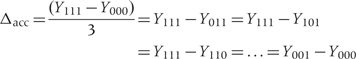
Under the accumulation hypothesis, the longer the time spent in a non-manual SEP, the lower the expected value of BMI, irrespective of the time point at which the SEP occurred. Hence, those in a manual SEP at all three time points would be expected to have a greater BMI than those in a manual SEP at any two time points who would in turn be expected to have a greater BMI than those in a manual SEP at any one time point, with those always in a non-manual SEP having the lowest BMI. If the outcome is independent of the timing of being in manual occupation, it follows that Y₀₀₁= Y₀₁₀= Y₁₀₀ and Y₀₁₁ = Y₁₀₁ = Y₁₁₀, where for simplicity here, and in the causal contrasts, we use Y to denote E(Y) and the suffix to denote the timing of exposure, e.g. suffix (001) indicating a trajectory where non-manual occupation was reported at the third time point only. If the outcome depends on the amount of exposure then Y₀₁₁ < Y₀₀₁ and Y₁₁₁ < Y₀₁₁. If it depends on it linearly then every trajectory can be represented by the total number of exposed periods, equal to Σ_jS_j (taking values between 0, always manual, and 3, always non-manual) that we call the lifetime SEP score. For every unit increase in this score, the change in mean BMI is assumed to be constant and equal to Δ_acc defined as

(3)

Assuming a direct and cumulative causal effect of SEP, Δ_acc would be the causal parameter of interest. It could be estimated by fitting the linear regression model:^1–3,5,6,9

(4)

where β corresponds to Δ_acc. The SEP indicators corresponding to different ages are summed to obtain a lifetime SEP score (Σ_j S_j) that takes values between 0 (always manual) and 3 (always non-manual).

Critical period model

Under the critical period hypothesis there are as many possible scenarios as there are time points. The one most investigated in life course epidemiology is the early life critical period hypothesis. In our example, this translates to a manual social class in childhood leading to greater expected BMI, irrespective of later SEP. Hence, it assumes that

(5)

Note that an asterisk indicates that SEP can take all possible values at that time point. Following the notation of Sampson et al.¹⁵ the theoretical causal contrast of interest would be the difference in BMI between those in the manual social class and those in the non-manual social class in childhood, averaging over later time points

(6)

This model assumes that only SEP in childhood has an effect on BMI, irrespective of the later SEP trajectory.

The equivalent expression for the early adulthood critical period hypotheses is:

(7)

and for the late adulthood critical period hypothesis:

(8)

The linear regression model corresponding to the early critical period is:

(9)

where β₁ corresponds to Δ_{early crit. period} in equation (6). Equivalent specifications of the other critical period models can be similarly specified. For instance, a model with β₂ only captures Δ_{early adult crit. period}.

Mobility model

The specification of the causal contrast implied by the social mobility hypothesis is the more complex of the three because there are different possible definitions of social mobility. First, we consider intra-generational (or adult) mobility as defined by Hallqvist et al.⁴ where any downwards (i.e. from non-manual = 1 to manual = 0) mobility in adulthood would be harmful to health (e.g. lead to an increase in BMI), and any upwards (i.e. from 0 to 1) mobility in adulthood would be beneficial, irrespective of early life social background. Thus,

(10)

The causal parameters of interest for the effects of down and upwards mobility would be

(11)

(12)

The linear regression model equivalent to this hypothesis is

(13)

where only transitions between periods 2 and 3 are relevant. Converting the D_j,j+1 and U_j,j+1 into S_j helps in understanding the parameter constraints that are implied by any given social mobility hypothesis. For instance, by specifying D_j,j+1 = S_j(1− S_j+1) and U_j,j+1 = (1−S_j)S_j+1 we can re-write equation (13) as

(14)

i.e. the expectation of Y is a function of the two adult SEP values and of their interaction.

Using the notation of equation (2), equation (14) could be re-written as

(15)

where β₂ = δ₂₃, β₃ = γ₂₃ with the constraint that θ₂₃ = −(δ₂₃ + γ₂₃) = −(β₂ +β₃).

An alternative model of social mobility assumes that all downward changes are equally harmful to health and all upward changes are equally beneficial. Thus, we assume that

(16)

i.e. same expected BMI in those with never changed SEP, and in those who moved from manual to non-manual at some point in their life time, in those who moved from non-manual to manual at some point in the life time. The causal parameters of interest would be

(17)

(18)

This general social mobility model does not specify the size of Δ_upwards relative to Δ_downwards or, equivalently, whether improving and then worsening one's position, as in Y₀₁₀ is better or worse than worsening and then improving it, as in Y₁₀₁.

The linear regression model equivalent to this latter hypothesis is:

(19)

Thus, equation (19) could be re-written as

(20)

where β₁ = δ, β₃ = γ, with the constraints that β₂ = (δ+γ) = (β₁ + β₃) and θ₁₂ = θ₂₃ = −β₂.

Model selection

The equations above show that different models relating the effects of SEP across the life course on a later outcome can be formulated in terms of alternative specifications of the regression model of Y on S₁, S₂, S₃ and their two-way interactions. The various constraints on the equality of parameter values explain how the same set of SEP values at the three time points can lead to very contradictory causal contrasts. For example, with regards to BMI we would expect Y₀₀₀ > Y₁₁₀ under the accumulation and both the early life and early adult critical period hypotheses, but under the two social mobility hypotheses, because of the constraint Y₀₀₀ = Y₁₁₁, we would expect BMI to reflect Y₀₀₀ < Y₁₁₀. This means that alternative hypotheses, due to the different sets of equality constraints required for each, can be formally tested by comparison to a saturated model.

Test for the accumulation hypothesis

If the accumulation of risk hypothesis defined in equation (3) were correct, we would expect—using the notation in (2)—that β₁ = β₂ = β₃ and that θ₁₂ = θ₂₃ = θ₁₃ = θ₁₂₃ = 0. This can be formally tested by performing a partial F-test between the saturated model with eight parameters and the simpler model on which these constraints are imposed (and which estimates only two parameters: α and β = β₁ = β₂ = β₃). The resulting test statistics are then compared with the F distribution with 6 and (N-8) degrees of freedom (df), where N is the sample size. Large P-values indicate that the restricted model is as good as the saturated model in fitting the data and therefore that the accumulation of risk hypothesis is supported by the data. However, before selecting any single hypothesis it is important to determine if other models also fit the data.

Test for the critical period hypothesis

To test the early life critical period hypothesis the parameter constraints, using the specification of the saturated model given in (2), would be β₂ = β₃ = θ₁₂ = θ₂₃ = θ₁₃= θ₁₂₃ = 0. The corresponding partial F-test statistic has [6, (N-8)] df and the interpretation of a resulting test would be as above, i.e. large P-values indicating consistency with the data.

Test for the social mobility hypotheses

The restricted model used to test the adult social mobility hypothesis has only three parameters: α, δ₂₃ and γ₂₃ with the constraints that η = δ₁₂ = γ₁₂ = ψ₁ = ψ₂ = 0, to be tested against the full model in equation (1) with df for the partial F-test equal to 5 and (N-8). Using the notation of equation (2) we would impose constraints θ₂₃ = −(β₂ + β₃), and β₁ = θ₁₂ = θ₁₃ = θ₁₂₃ = 0, with the same df as above.

The social mobility hypothesis with time invariant effects would again estimate three parameters, namely α and δ = δ₁₂ = δ₂₃ and γ = γ₁₂ = γ₂₃ with constraints ψ₁ = ψ₂ = η = 0. Alternatively using the notation in equation (2) the constraints would be β₂ = (β₁ + β₃), θ₁₂ = θ₂₃ = −β₂ and θ₁₃ = θ₁₂₃ = 0. With either specification the partial F-test statistics would have [5, (N-8)] df.

Results

For the purpose of the example considered here the analyses were stratified by sex. Approximately a third (men 31.2%, women 33.7%) stayed in the non-manual group at all the three time points (Table 2). More than twice the proportion of men remained in manual occupation from childhood to age 43 years compared with women (26.5% and 13.0%, respectively). Trajectories that indicated change in SEP through the life course were dominated by those who changed from a childhood manual group to non-manual group by age 26 years and remained there at age 43 years (29% for women and 17% for men). Those women who were always in the non-manual SEP group had a consistently lower BMI than those who were in the manual group in childhood or in the manual group at age 43 years. Among men the highest BMI means were observed in three of the four trajectories that include childhood manual SEP.

Table 2.

Distribution of socioeconomic trajectories within women and men in the MRC National Survey, and observed and predicted mean BMI (standard error) according to different hypotheses, by SEP permutation and sex

						Mean BMI predicted from regression coefficients estimated imposing constraints implied by alternative life course hypotheses
	SEPa						Critical periodb			Social mobility
Sex	SEP1	SEP2	SEP3	N (%)	Observed mean BMI in 1999	Accumulation	t1	t2	t3	Adult	Any mobility
Women				n = 1088
	0	0	0	141 (13.0)	28.7 (0.5)	29.2 (0.3)	28.1 (0.2)	28.1 (0.3)	28.7 (0.3)	27.1 (0.2)	26.8 (0.2)
	1	0	0	20 (1.8)	27.5 (1.1)	28.2 (0.2)	26.4 (0.3)	28.1 (0.3)	28.7 (0.3)	27.1 (0.2)	27.8 (0.5)
	0	1	0	88 (8.1)	29.1 (0.7)	28.2 (0.2)	28.1 (0.2)	27.1 (0.2)	28.7 (0.3)	28.8 (0.5)	28.6 (0.4)
	0	0	1	80 (7.4)	27.8 (0.7)	28.2 (0.2)	28.1 (0.2)	28.1 (0.3)	26.9 (0.2)	27.6 (0.5)	27.6 (0.3)
	1	1	0	40 (3.7)	28.3 (0.8)	27.3 (0.2)	26.4 (0.3)	27.1 (0.2)	28.7 (0.3)	28.8 (0.5)	27.8 (0.5)
	1	0	1	35 (3.2)	27.1 (0.9)	27.3 (0.2)	26.4 (0.3)	28.1 (0.3)	26.9 (0.2)	27.6 (0.5)	28.6 (0.4)
	0	1	1	317 (29.1)	27.6 (0.3)	27.3 (0.2)	28.1 (0.2)	27.1 (0.2)	26.9 (0.2)	27.1 (0.2)	27.6 (0.3)
	1	1	1	367 (33.7)	26.0 (0.2)	26.3 (0.2)	26.4 (0.3)	27.1 (0.2)	26.9 (0.2)	27.1 (0.2)	26.8 (0.2)
Men				n = 1104
	0	0	0	292 (26.5)	27.8 (0.3)	27.9 (0.2)	27.8 (0.2)	27.7 (0.2)	27.5 (0.2)	27.3 (0.1)	27.2 (0.2)
	1	0	0	61 (5.5)	27.2 (0.6)	27.6 (0.1)	26.8 (0.2)	27.7 (0.2)	27.5 (0.2)	27.3 (0.1)	26.8 (0.3)
	0	1	0	27 (2.5)	26.3 (0.7)	27.6 (0.1)	27.8 (0.2)	27.1 (0.2)	27.5 (0.2)	26.6 (0.6)	27.4 (0.4)
	0	0	1	125 (11.3)	27.8 (0.3)	27.6 (0.1)	27.8 (0.2)	27.7 (0.2)	27.2 (0.2)	27.7 (0.3)	27.8 (0.2)
	1	1	0	22 (2.0)	26.9 (0.9)	27.2 (0.1)	26.8 (0.2)	27.1 (0.2)	27.5 (0.2)	26.6 (0.6)	26.8 (0.4)
	1	0	1	45 (4.1)	27.5 (0.6)	27.2 (0.1)	26.8 (0.2)	27.7 (0.2)	27.2 (0.2)	27.7 (0.3)	27.4(0.4)
	0	1	1	188 (17.0)	28.0 (0.3)	27.2 (0.1)	27.8 (0.2)	27.1 (0.2)	27.2 (0.2)	27.3 (0.2)	27.8 (0.2)
	1	1	1	344 (31.2)	26.6 (0.2)	26.9 (0.2)	26.8 (0.2)	27.1 (0.2)	27.2 (0.2)	27.3 (0.2)	27.2 (0.2)

Bold numbers correspond to close observed and predicted means in the more frequent trajectories.

^a0 refers to manual SEP, 1 refers to non-manual SEP.

^bCritical period at time t₁, t₂, t₃ corresponds to ages 4, 26 and 43 years.

Alternative linear regression models were fitted to the data corresponding to the hypotheses for the effect of social class over the life course, described in the Methods section. The mean values of BMI for each combination of values of S₁, S₂ and S₃ predicted by these models are displayed in Table 2 next to the observed mean values.

The accumulation of risk model provides the best fit to the data for women, since consideration of the F-statistics (Table 3) shows that only for this model was no significant difference from the saturated model observed (P = 0.214). The best predictions from the accumulation model were for the most frequent trajectories (Table 2). For men the early life critical period model provides the best fit (P = 0.359). In terms of prediction, the trajectory (0, 1, 0) was an exception as this group had the greatest disparity between observed (26.3 kg/m²) and expected mean BMI (27.8 kg/m²), but there were very few men (n = 27) who experienced this trajectory. For both men and women, the accumulation of risk model indicated significant decreasing linear trends in BMI with increasing SEP score [β (95% CI) men: −0.34 (−0.54 to −0.14) kg/m², P = 0.001; women: −0.95 (−1.26 to −0.63) kg/m², P < 0.001]. Hence, if only considering this model, we might conclude there is evidence for the accumulation model. However, men who had trajectories (0, 0, 1) or (1, 0, 0), both with an SEP score of 1, differed in their observed means (27.8 vs 27.2 kg/m²) by more than the estimated effect of 0.34 kg/m² per unit decrease in the lifetime SEP score (Table 2). This is consistent with our finding that the best fitting model for men was the childhood critical period model, with an effect of non-manual class on BMI of −0.98 (−1.46 to −0.50) kg/m², P < 0.001.

Table 3.

Series of full and partial F-tests for different contrasts according to different hypotheses

	Model tested: using notation corresponding		Partial F-test against saturated model
Hypothesis	Equation (1)	Equation (2)	df	F-statistic	P-value
Women
No effect	α = δ12 = γ12 = δ23 = γ23 = ψ1 = ψ2 = η = 0	β1 = β2 = β3 = θ12 = θ23 = θ13 = θ123 = 0	7, 1080	6.26	<0.001
Accumulation of risk	δ12 = γ12 = δ23 = γ23 = ψ1 = ψ2 = 0; η = 1	β1 = β2 = β3; θ12 = θ23 = θ13 = θ123 = 0	6, 1080	1.39	0.214
Critical perioda
t1	δ23 = γ23 = ψ1 = ψ2 = η = 0	β2 = β3 = θ12 = θ23 = θ13 = θ123 = 0	6, 1080	2.57	0.018
t2	δ23 = γ23 = ψ1 = ψ2 = 0	β1 = β3 = θ12 = θ23 = θ13 = θ123 = 0	6, 1080	5.97	<0.0001
t3	δ12 = γ12+ψ1 = ψ2 = η = 0	β1 = β2 = θ12 = θ23 = θ13 = θ123 = 0	6, 1080	3.36	0.003
Social mobility
Adult	η = δ12 = γ12 = ψ1 = ψ2 = 0	θ23 = −(β2+ β3), β1 = θ12 = θ13 = θ123 = 0	5, 1080	6.42	<0.0001
Any mobility	δ = δ12 = δ23,γ = γ12 = γ23 ψ1 = ψ2 = η = 0	β2 = (β1 + β3), θ12 = θ23 = −β2, θ13 = θ123 = 0	5, 1080	5.97	<0.0001
Men
No effect	α = δ12 = γ12 = δ23 = γ23 = ψ1 = ψ2 = η = 0	β1 = β2 = β3 = θ12 = θ23 = θ13 = θ123 = 0	7, 1096	3.25	0.002
Accumulation of risk	δ12 = γ12 = δ23 = γ23 = ψ1 = ψ2 = 0, η = 1	β1 = β2 = β3; θ12 = θ23 = θ13 = θ123 = 0	6, 1096	1.99	0.060
Critical perioda
t1	δ23 = γ23 = ψ1 = ψ2 = η = 0	β2 = β3 = θ12 = θ23 = θ13 = θ123 = 0	6, 1096	1.10	0.359
t2	δ23 = γ23 = ψ1 = ψ2 = 0	β1 = β3 = θ12 = θ23 = θ13 = θ123 = 0	6, 1096	2.66	0.015
t3	δ12 = γ12 + ψ1 = ψ2 = η = 0	β1 = β2 = θ12 = θ23 = θ13 = θ123 = 0	6, 1096	3.54	0.002
Social mobility
Adult	η = δ12 = γ12 = ψ1 = ψ2 = 0	θ23 = −(β2+ β3), β1 = θ12 = θ13 = θ123 = 0	5, 1096	3.94	0.002
Any mobility	δ = δ12 = δ23, γ = γ12 = γ23, ψ1 = ψ2 = η = 0	β2 = (β1 + β3), θ12 = θ23 = −β2, θ13 = θ123 = 0	5, 1096	3.28	0.006

^aCritical period at time t₁, t₂, t₃ corresponds to ages 4, 26 and 43 years.

The social mobility models showed a particularly poor fit for both sexes as it is significantly different from the saturated model (P < 0.01). The adult social mobility model estimated for women virtually no change in BMI for upwards adult SEP mobility [γ₂₃ (95% CI): 0.48 (−0.57 to 1.52) kg/m², P = 0.372], and some increase in BMI for downwards mobility [δ₂₃ (95% CI): 1.70 (0.70 to 2.70) kg/m², P = 0.001], and for men no significant effects of changing adult SEP [γ₂₃: 0.34 (−0.318 to 1.01) kg/m², P = 0.308 and δ₂₃: −0.78 (−1.94 to 0.38) kg/m², P = 0.187]. In women, the more general social mobility model estimated both upward and downward change in SEP to be associated with increases in BMI [γ: 0.84 (0.19 to 1.48) kg/m², P = 0.011 and δ: 0.97 (0.10 to 1.83) kg/m², P = 0.028]. This was due to the generally higher weight for women in all trajectories compared with those women who remained in the non-manual trajectory throughout. In men, the same model estimated some minor increase in weight for an upward change, and no change in weight for a downward change in SEP [γ: 0.59 (0.09 to 1.09) kg/m², P = 0.020 and δ: −0.41 (−1.10 to 0.27) kg/m², P = 0.239]. This was due to an upward change in SEP only being possible by being in a manual SEP beforehand and to the strong effect of childhood manual SEP on BMI in men.

Discussion

In this article, we have examined models that are frequently discussed in the literature^3,4,6–8,16 and parameterized them so that they could be viewed as alternative nested specifications of a more general (saturated) model. We have done this within a linear regression framework but it can be easily extended to any generalized linear model, e.g. Poisson or logistic, with the only difference concerning the test statistics used to compare the model specifications. While partial F-tests should be used in linear regression to compare nested models, the likelihood ratio test or one of its approximations would be used with generalized linear models.¹⁷ We have focused on mean outcomes to illustrate the method, other features of the outcome distributions, such as the median or 25th percentile, may equally have been used. We have shown how analyses that only consider the association of a cumulative score with a later outcome may result in a misleading conclusion.

Our analyses of the MRC NSHD data found that for the BMI of women at age 53 years an accumulation of risk model for adverse social circumstances seemed to be most appropriate. This supports results previously found for women in this study and others.^18,19 In contrast, for men our results suggest that childhood was a critical period for adult BMI. This is in line with previous reports in the literature.^18,19 If we had not considered the whole spectrum of alternative model specifications, we might have concluded that the data on men were consistent with the accumulation of risk hypothesis, because the lifetime SEP score parameter actually captured the effect of the childhood critical period (its estimated coefficient, 0.979, being about three times that for the lifetime score, 0.336). We might have also concluded that the data on women were consistent with one of the social mobility models, given the significance of the γ and δ parameters.

In general, results based on a lifetime score may be driven by particular combinations of values over the three time points, these obviously being specific to the period and place where the data were collected. For example, in this study the majority of those with a cumulative score of 2 had trajectory (0, 1, 1) due to the considerable upward inter-generational mobility in this British post-war cohort. Re-weighting the social class indicator by the prevalence of that social class has been used to address the issue of the changing socioeconomic distribution over time,⁶ although this will lead to more complex variance structures. The problems surrounding the use and interpretation of lifetime SEP scores remain. Their popularity when dealing with three or more time-changing indicators of social class may be due in part to concerns regarding multi-collinearity. However, unless the binary indicators are measured very closely in time this is unlikely to be an issue.

Our proposed methods work for both critical period and accumulation hypotheses even as the number of time points increases beyond three. This is because the prior hypothesis will reduce the dimensionality of the data when testing a critical period model, while with the accumulation model one would simply sum the SEP indicators across time points to generate an overall score. However, the method would not generalize to more than three time points for the social mobility model. In this case the model should be simplified, or alternatively latent variable/class modelling could be used to define the main social trajectories.²⁰ Bayesian information criteria or Akaike's information are fairly established criteria for assessing model fit in this context. While our method could handle more time points, the challenge would be to have a study large enough to enable us to test the different life course models—all causal contrasts rely on equality of effects of other time points, and the larger the study the larger the power to detect small and meaningful differences in effect between trajectories/time points.

We have introduced a new parameterization for mobility models. Such parameterizations in terms of change, clarify algebraically what mobility models mean in a given study setting. The definitions of inter- and intra-generational mobility will depend on which time points are used in a particular study, the number of childhood and adult measurements. Our results have highlighted two issues in relation to the mobility models. First, mobility is conditional on the selected starting point—for example being born in a manual environment—and therefore results are to be interpreted accordingly. Second, we can only test for the presence of a mobility model if the data include sufficient changes from manual to non-manual occupation, and vice versa. Related to this, interaction terms are part of the specification of the mobility models and there may not be sufficient power to detect such interactions. Lack of power may also limit the ability to extend models to incorporate larger numbers of SEP trajectories as discussed above.

In reality, the processes operating across the life course may not conform to any of the causal models specified here and so it may be unrealistic to expect to disentangle explicitly such effects in practice. For example, the analyses were carried out under the assumption that these are representative of all participants, and that it is valid to assume that individuals with missing scores have remained in the same category at a later time point. Both these assumptions are debatable. Also, the current article has ignored issues related to uncertainty in assigning a given value of social class at a given point in time. For instance, it may be that the measurement errors associated with assigning SEP are much higher for adults than for their fathers, with resulting larger effects for childhood SEP. If we had data with more time points, then the correlations of SEP between two subsequent measurements would help to deal with measurement error issue (assuming non-differential errors). But correlations of SEP over time may lead to certain trajectories being very rare and hinder the analysis.

It is highly advantageous to have an understanding of the biological mechanisms underlying the effect of exposures on specific health outcomes upon which to base the statistical modelling. This may lead to a different specification of the mobility model than is used here. However, our approach highlights that the researcher should not adopt an a priori hypothesis without testing to see if other models fit the data equally well.

With more complex causal structures and/or more social class categories or indicators, latent socioeconomic constructs at each time point could be used to model pathways explicitly.^21,22 Although the latent variable modelling has more apparent flexibility in terms of integrating over missing information using maximum likelihood, it still relies on assumptions on how these various SEP indicators are related and crucially on the structure of the available data, as discussed in De Stavola et al.²³ among others. It may be more appropriate to refer to sensitive periods, where there is more scope for modification or reversal of changes outside that time, in contrast with critical periods where developmental changes are irreversible.⁷ In such cases, where the model fit tests indicate more than one model is plausible, further equality constraints could be relaxed to define a combined model, which can then be tested. Simulation studies may be used to see how often one model structure is preferred over another.

In this article, we have adopted a counterfactual framework to outline the causal hypotheses however there remains the issue of using observational data to infer causality.²⁴ We have used ‘causal contrast’ to refer to the parameter of interest. More broadly it is important to consider the potential for confounding, such as due to exogenous events between time points, and to consider the possibility for reverse causality (for instance, a chronic condition associated with high BMI that leads to a lowering of SEP from childhood to adulthood). As Kaufman comments, while rigid conditions can be applied to the models to simplify such issues, such as requiring monotonicity of effects, many contrasts may remain unidentifiable or many apparent patterns may be artefacts of the chosen contrasts.²⁵ In summary, regardless of which model is selected, issues of measurement error, missing data, survival bias, confounding factors are inevitable in life course studies and hence results may still be biased and thus caution is required in their interpretation.

We have illustrated how analyses that simply report effects of an overall score based on its statistical significance may produce misleading or incomplete results that do little to help the understanding of how life course trajectories affect health. While Hallqvist et al.⁴ found that testing different models against the null hypothesis was unable to disentangle empirically causal processes, we have shown that our alternative model fit approach can be used to distinguish different life course hypotheses, given the assumption of no measurement errors and provided the study has sufficient power. Specifically we recommend comparing a set of nested models—each corresponding to the accumulation, critical period and effect modification hypotheses—to an all-inclusive (saturated) model. This approach can provide a formal and clearer understanding of the relative merits of these alternative hypotheses.

Funding

Medical Research Council.

References

- 1.Davey Smith G, Hart C, Blane D, Gillis C, Hawthorne V. Lifetime socioeconomic position and mortality: prospective observational study. Br Med J. 1997;314:547–52. doi: 10.1136/bmj.314.7080.547. [DOI] [PMC free article] [PubMed] [Google Scholar]
- 2.Wamala SP, Lynch J, Kaplan GA. Women's exposure to early and later life socioeconomic disadvantage and coronary heart disease risk: the Stockholm Female Coronary Risk Study. Int J Epidemiol. 2001;30:275–84. doi: 10.1093/ije/30.2.275. [DOI] [PubMed] [Google Scholar]
- 3.Singh-Manoux A, Ferrie JE, Chandola T, Marmot M. Socioeconomic trajectories across the life course and health outcomes in midlife: evidence for the accumulation hypothesis? Int J Epidemiol. 2004;33:1072–79. doi: 10.1093/ije/dyh224. [DOI] [PubMed] [Google Scholar]
- 4.Hallqvist J, Lynch J, Bartley M, Lang T, Blane D. Can we disentangle life course processes of accumulation, critical period and social mobility? An analysis of disadvantaged socio-economic positions and myocardial infarction in the Stockholm Heart Epidemiology Program. Soc Sci Med. 2004;58:1555–62. doi: 10.1016/S0277-9536(03)00344-7. [DOI] [PubMed] [Google Scholar]
- 5.Naess O, Claussen B, Thelle DS, Davey Smith G. Cumulative deprivation and cause specific mortality. A census based study of life course influences over three decades. J Epidemiol Community Health. 2004;58:599–603. doi: 10.1136/jech.2003.010207. [DOI] [PMC free article] [PubMed] [Google Scholar]
- 6.Lawlor DA, Davey Smith G, Patel R, Ebrahim S. Life-course socioeconomic position, area deprivation, and coronary heart disease: findings from the British Women's Heart and Health Study. Am J Public Health. 2005;95:91–97. doi: 10.2105/AJPH.2003.035592. [DOI] [PMC free article] [PubMed] [Google Scholar]
- 7.Kuh D, Ben-Shlomo Y. A Life Course Approach to Chronic Disease Epidemiology. Oxford: Oxford University Press; 2004. [PubMed] [Google Scholar]
- 8.Kuh D, Ben-Shlomo Y, Lynch J, Hallqvist J, Power C. A glossary for life course epidemiology. J Epidemiol Community Health. 2003;57:778–83. doi: 10.1136/jech.57.10.778. [DOI] [PMC free article] [PubMed] [Google Scholar]
- 9.Power C, Manor O, Matthews S. The duration and timing of exposure: effects of socioeconomic environment on adult health. Am J Public Health. 1999;89:1059–65. doi: 10.2105/ajph.89.7.1059. [DOI] [PMC free article] [PubMed] [Google Scholar]
- 10.Barker DJP. Fetal and Infant Origins of Adult Disease. London: British Medical Journal; 1992. [Google Scholar]
- 11.Power C, Manor O, Matthews S. Child to adult socioeconomic conditions and obesity in a national cohort. Int J Obes Relat Metab Disord. 2003;27:1081–86. doi: 10.1038/sj.ijo.0802323. [DOI] [PubMed] [Google Scholar]
- 12.Hardy R, Wadsworth MEJ, Kuh D. The influence of childhood weight and socioeconomic status on change in adult body mass index in a British national birth cohort. Int J Obesity. 2000;24:1–10. doi: 10.1038/sj.ijo.0801238. [DOI] [PubMed] [Google Scholar]
- 13.Wadsworth ME, Butterworth SL, Hardy RJ, et al. The life course prospective design: an example of benefits and problems associated with study longevity. Soc Sci Med. 2003;57:2193–205. doi: 10.1016/s0277-9536(03)00083-2. [DOI] [PubMed] [Google Scholar]
- 14.Greenland S, Brumback B. An overview of relations among causal modelling methods. Int J Epidemiol. 2002;31:1030–37. doi: 10.1093/ije/31.5.1030. [DOI] [PubMed] [Google Scholar]
- 15.Sampson RJ, Sharkey P, Raudenbush SW. Durable effects of concentrated disadvantage on verbal ability among African-American children. Proc Natl Acad Sci USA. 2008;105:845–52. doi: 10.1073/pnas.0710189104. [DOI] [PMC free article] [PubMed] [Google Scholar]
- 16.Manor O, Matthews S, Power C. Health selection: the role of inter- and intra-generational mobility on social inequalities in health. Soc Sci Med. 2003;57:2217–27. doi: 10.1016/s0277-9536(03)00097-2. [DOI] [PubMed] [Google Scholar]
- 17.Clayton D, Hills M. Statistical Models in Epidemiology. Oxford: Oxford University Press; 1993. [Google Scholar]
- 18.Blane D, Hart CL, Smith GD, Gillis CR, Hole DJ, Hawthorne VM. Association of cardiovascular disease risk factors with socioeconomic position during childhood and during adulthood. Br Med J. 1996;313:1434–38. doi: 10.1136/bmj.313.7070.1434. [DOI] [PMC free article] [PubMed] [Google Scholar]
- 19.Langenberg C, Hardy R, Kuh D, Brunner E, Wadsworth M. Central and total obesity in middle aged men and women in relation to lifetime socioeconomic status: evidence from a national birth cohort. J Epidemiol Community Health. 2003;57:816–22. doi: 10.1136/jech.57.10.816. [DOI] [PMC free article] [PubMed] [Google Scholar]
- 20.Muthén L, Muthén B. Mplus: Statistical Analysis with Latent Variables. Los Angeles, CA: Muthén and Muthén; 1998. [Google Scholar]
- 21.Richards M, Sacker A. Lifetime antecedents of cognitive reserve. J Clin Exp Neuropsychol. 2003;25:614–24. doi: 10.1076/jcen.25.5.614.14581. [DOI] [PubMed] [Google Scholar]
- 22.Singh-Manoux A, Richards M, Marmot M. Socioeconomic position across the lifecourse: how does it relate to cognitive function in mid-life? Ann Epidemiol. 2005;15:572–78. doi: 10.1016/j.annepidem.2004.10.007. [DOI] [PubMed] [Google Scholar]
- 23.De Stavola BL, Nitsch D, Dos SSI, et al. Statistical issues in life course epidemiology. Am J Epidemiol. 2006;163:84–96. doi: 10.1093/aje/kwj003. [DOI] [PubMed] [Google Scholar]
- 24.Kaufman JS, Cooper RS. Seeking causal explanations in social epidemiology. Am J Epidemiol. 1999;150:113–20. doi: 10.1093/oxfordjournals.aje.a009969. [DOI] [PubMed] [Google Scholar]
- 25.Kaufman JS. Specifying counterfactual contrasts for the health effects of socioeconomic position at different points in the life-course. Am J Epidemiol. 2008;167:S137. [Google Scholar]