Estimating Local Ancestry in Admixed Populations

Abstract

Large-scale genotyping of SNPs has shown a great promise in identifying markers that could be linked to diseases. One of the major obstacles involved in performing these studies is that the underlying population substructure could produce spurious associations. Population substructure can be caused by the presence of two distinct subpopulations or a single pool of admixed individuals. In this work, we focus on the latter, which is significantly harder to detect in practice. New advances in this research direction are expected to play a key role in identifying loci that are different among different populations and are still associated with a disease. We evaluated current methods for inference of population substructure in such cases and show that they might be quite inaccurate even in relatively simple scenarios. We therefore introduce a new method, LAMP (Local Ancestry in adMixed Populations), which infers the ancestry of each individual at every single-nucleotide polymorphism (SNP). LAMP computes the ancestry structure for overlapping windows of contiguous SNPs and combines the results with a majority vote. Our empirical results show that LAMP is significantly more accurate and more efficient than existing methods for inferrring locus-specific ancestries, enabling it to handle large-scale datasets. We further show that LAMP can be used to estimate the individual admixture of each individual. Our experimental evaluation indicates that this extension yields a considerably more accurate estimate of individual admixture than state-of-the-art methods such as STRUCTURE or EIGENSTRAT, which are frequently used for the correction of population stratification in association studies.

Introduction

Recent advances in genotyping technologies have opened up unprecedented opportunities to improve our understanding of complex diseases through disease association studies. In these studies, a population of cases and controls are genotyped across the genome, and the allele frequencies are compared across these two groups. Currently, in a typical study, hundreds of thousands of single-nucleotide polymorphisms (SNPs) are genotyped for thousands of individuals.¹ These numbers are expected to grow in the coming years because of the constant improvements in genotyping technologies.¹

A significant discrepancy between the allele frequencies in the cases and the controls gives evidence for an association between the SNP and the phenotype and therefore links the SNP to the disease. However, a growing concern is that many of the associations found are due to confounding effects. In particular, if the cases and the controls are not sampled from the same population, many spurious associations will be discovered because the two populations might have different allele frequencies at a SNP regardless of the disease status.^2–10 This bias can be observed in diseases that are more prevalent in one population than in another. In such cases, the collection of the cases is a biased sample of the population.

Various methods have been proposed to deal with population substructure in association studies.^2,11 One of the most intuitive approaches is to first find the population substructure within the cases and the controls by using a clustering algorithm such as STRUCTURE¹² and then to correct it by using regression or other methods that take the subpopulation variable into account.¹³ The clustering algorithms need to be accurate enough, so that the signal obtained from the difference in population substructure will be weaker than the signal obtained from the difference in the disease status.

The problem of inferring the population substructure is especially challenging when recently admixed populations are involved. In these populations (e.g., African Americans and Latinos), two or more ancestral populations have been mixing for a relatively small number of generations, resulting in a new population in which the ancestry of every individual can be explained by different proportions of the original populations. Because of recombination events, even within the DNA of a single individual, different regions of the genome could originate from different ancestral populations. This adds to the complexity of the problem of finding the ancestral information of an individual because in nonadmixed populations, the whole genome can be used as evidence for the population membership of an individual, whereas in the admixed case, the genome of each individual is fragmented into shorter regions of different ancestry. It is therefore challenging to find the ancestral information of these individuals and, in particular, to find the locus-specific ancestries.

An accurate inference of locus-specific ancestry in admixed populations could lead to improved analysis of studies based on admixture mapping. In these studies, a set of cases from a recently admixed population is genotyped, and the genome is scanned for regions in which the proportions of ancestral populations are significantly different than the rest of the genome.^14,15 Unfortunately, most of the current methods for inference of locus-specific ancestral information^12,16–18 do not scale to large datasets. The only existing method that copes with large datasets is SABER,¹⁹ which is based on an extension of a Hidden Markov Model²⁰ that deals with local haplotype blocks.

Here, we propose a new method, LAMP (Local Ancestry in adMixed Populations), for de novo estimation of the locus-specific ancestry in recently admixed populations (see Figure 1). Our method is based on the observation that previous methods that use a Hidden Markov Model, or extensions of it, are set to infer a very large set of parameters, including the exact position of the recombination events, making the search over the parameter space infeasible. Instead, our method operates on sliding windows of contiguous SNPs. We first calculate an optimal window length. Next, we use a clustering algorithm that operates on these windows and estimates each individual's ancestry. We then use a majority vote for each SNP, over all windows that overlap with the SNP, in order to decide the most likely ancestral populations at the SNP. This simple approach has two advantages over previous ones. First, we show analytically that the estimates of the algorithm are asymptotically correct across the entire genome. Second, it optimizes fewer parameters than previous methods, and hence the optimization is much faster and more robust than previous methods.

Figure 1.

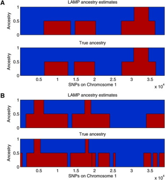
Two Individuals in an Admixed Population

Ancestries predicted by LAMP (top panel) and true ancestries (bottom panel) are shown for each individual (A and B). As shown in the figure, the ancestries (represented by red and blue) vary across the genome, and LAMP performs well in inferring the ancestry at each location.

We tested LAMP extensively on various datasets of admixed populations generated from the HapMap resource. Our simulations show that LAMP is significantly more accurate than state-of-the-art methods such as SABER and STRUCTURE. In addition, LAMP is highly efficient, with a running time that is about 200 times faster than SABER and about 10⁴ times faster than STRUCTURE. The efficiency of LAMP allows us to estimate ancestries across the genome in several hours on a single computer.

An additional advantage of LAMP is that unlike previous methods, such as SABER, it does not require the ancestral genotypes to infer the locus-specific ancestries (though it can take advantage of these, if available). This might be crucial when the ancestral genotypes cannot be typed or are unknown. For instance, if one studies the population genetics of populations in remote geographic locations where historical admixing has not been recorded, a method such as LAMP could be used to reveal such recent admixing. Furthermore, even in cases where the history of admixing is known, it is not always possible to genotype all the ancestral populations because some of the subpopulations have become extinct and some have entirely mixed with other populations. On the other hand, as genotypes of major population groups become available, it would be beneficial to use LAMP-ANC (ANC: ancestral), which can take advantage of the pure genotypes.

Surprisingly, we find that in many cases where LAMP does not receive the genotypes of the ancestral populations as input, it performs considerably better than SABER. In particular, on a simulated dataset of African Americans, when measuring the percentage of individuals that are predicted with an accuracy of at least 90%, LAMP achieves high accuracies on 90% of the individuals, whereas SABER and STRUCTURE achieve less than 10%.

Finally, we used LAMP to estimate the individual admixture and showed empirically that this results in much more accurate estimates than methods such as STRUCTURE¹² or EIGENSTRAT.² This reduction in errors might be used to considerably reduce the rate of spurious association results in disease association studies.

Material and Methods

The inference of locus-specific ancestry depends on the mathematical model representing the mixing process of the populations. We will first describe the model assumptions and then describe the inference algorithm under the model.

Model Assumptions

We assume that there are K ancestral populations A₁, …, A_K that have been mixing for g generations. If the populations have mixed at different times, then g is taken to be an upper bound on the number of generations since the beginning of admixture. The fraction of population A_i in the ancestral population that we call the admixture fraction is α_i, where $\sum _i{\mathit{\alpha }}_i=1$. We assume for convenience that α₁ ≥ α₂… ≥ α_K. In each generation, we assume random mating within the combined pool of the k populations. We denote the recombination rate at position j by r_j. Note that r_j is the recombination rate at position j at a specific meiosis (one generation), and not through history. We model the transmission of a chromosome from a parent to a child by walking along the chromosome from the 5′ end to the 3′ end, with crossovers between chromosomes occurring as a Poisson process with rate r_j.²¹ For simplicity of the presentation, we will assume a uniform recombination rate, i.e., that r = r_j for every position j. The algorithm and analysis remain qualitatively the same when applied to nonuniform recombination rates.

We denote the genotype data of individual i at position j as g_ij, where g_ij ∈ {0, 1, 2} is the minor allele count at that position. At position j, the two alleles of individual i have descended from one or two of the K ancestral populations. We denote by $a_{\mathit{ij}}^p$ ∈ {0, 0.5, 1} the fraction of alleles descended from population p at position j in individual i. The quantities $a_{\mathit{ij}}^p$ are unknown; the objective of this paper is to present a method LAMP that accurately estimates these quantities.

The LAMP Framework

In this work, we consider a recently admixed population in which the number of generations g since the beginning of the mixing is small. Therefore, we expect the total number of recombinations in these g generations to be small, as well. The resulting chromosomes are mosaics of the k populations, where the ancestral breakpoints in which the chromosome ancestry changes from one population to the other are determined by the recombination events.

We assume that the quantities g, α_i, and r are known for the admixed population. The basic idea in LAMP is to estimate the ancestries of the individuals in a sliding window that spans l sites. We term l the length of the window. The choice of the length l will be discussed later. Intuitively, if l is small enough, and the number of generations g is not too large, a typical window of length l will have almost no recombination events throughout history, and therefore almost no breakpoints. Therefore, within each window, it is reasonable to use an inference algorithm that assigns the sequence of genotypes in the window to one or two of the populations under the assumption that there are no breakpoints in any of the chromosomes. The latter is a simple clustering problem, although the accuracy of the inference in a given window improves when the number of SNPs l in the window increases. We therefore search for a window length l that is short enough so that most individuals have no breakpoints and large enough so that there is enough information to correctly cluster the individuals within the window. This procedure is repeated by sliding the window to cover all the SNPs on the genome. The windows that overlap a SNP are then combined into a single solution with a majority vote for the ancestry assignment. We note that unlike previous methods (e.g., SABER¹⁹ or STRUCTURE¹²), we are not attempting to estimate the exact positions of the breakpoints; instead, we are trying to minimize the errors in the locus-specific ancestry prediction across the genome.

The LAMP algorithm works as follows. We first find the optimal window length on the basis of the parameters g, α_i, and r. Then, we use a clustering algorithm that operates on a window and estimates for each individual i, and for each ancestral populations A_j, A_k, the probability $p_{\mathit{jk}}^i$ for individual i to have one chromosome descended from population A_j at this window and another descended from population A_k. We then use a majority vote for each SNP, over all windows that overlap with the SNP, in order to decide the most likely ancestral populations at the SNP. As we argue below, even though this scheme optimizes less parameters than previous methods, such as SABER, or a regular hidden Markov model (HMM), we show analytically and empirically that the estimates of the algorithm are asymptotically correct across the entire genome.

Estimating the Ancestry in a Single Window

We assume that none of the individuals have a breakpoint within a window and estimate a single ancestral origin for each individual across the length of the window. This assumption is largely true if the length of the window is determined correctly (see Choosing the Window Length, as well as Estimate of Window Length in the Appendix). We further assume that the values α₁, …, α_K are known. These values are the admixture fractions of each of the populations across the whole genome, and they can be estimated with existing tools such as STRUCTURE.¹² In the Results section, we show that our method is robust to reasonable inaccuracies in the estimates of α₁, …, α_K.

Clustering Algorithm

We assume that subpopulation A_i has minor allele frequencies $\overrightarrow{f_i}=f_{i1},\dots ,f_{\mathit{in}}$ for n SNPs in a given window of length l and that the different SNPs in the window are independent. The latter assumption can be achieved in practice by the greedy removal of SNPs having a high correlation coefficient (r² > 0.1) from the window. We look for a classification function $\mathit{\theta }:I\to {\{1,\dots ,K\}}^2$, where I is the set of individuals and the range corresponds to the possible pairs of subpopulations. In particular, we write θ(i) = (θ₁(i), θ₂(i)) to denote the ancestries of the two chromosomes of individual i in the current window. We use a clustering algorithm known as Iterated Conditional Modes (ICM)²² to find an optimal classification of each individual in terms of the likelihood. For increased efficiency in the running time, we seed the algorithm with an initial classification as described in the Initializing the Clusters section.

The updates in the ICM algorithm differ from those in a traditional expectation maximization (EM) method only in the E step. In the latter, the E step consists of obtaining the expected classification θ, given the values $\overrightarrow{f_i}$. This would provide fractional class membership for each individual i. However, because we assume that the initial classification provides a reasonable solution, we find the maximum aposteriori estimate of θ as shown below. For brevity, we use $G_i$ to refer to the genotype (g_i1, …, g_in) of the individual i.

$$\begin{array}{c}\widehat{\mathit{\theta }}\left(i\right)={\text{argmax}}_{A_s{A}_t\in {\{1,\dots ,K\}}^2}\mathrm{Pr}[\mathit{\theta }\left(i\right)=A_s{A}_t|\overrightarrow{f_1},\dots ,\overrightarrow{f_K},G_i]\\ ={\text{argmax}}_{A_s{A}_t\in {\{1,\dots ,K\}}^2}\mathrm{Pr}\left[G_i\right|\overrightarrow{f_1},\dots ,\overrightarrow{f_K},\mathit{\theta }\left(i\right)=A_s{A}_t]\cdot \mathrm{Pr}[\mathit{\theta }\left(i\right)=A_s{A}_t|\overrightarrow{f_1},\dots ,\overrightarrow{f_K}]\end{array}$$ (1)

Because α₁, …, α_K are known, under the assumption of random mating, we can estimate the first term Pr $[\mathit{\theta }\left(i\right)=A_s{A}_t|\overrightarrow{f_1},\dots ,\overrightarrow{f_K}]$ as Pr[θ(i) = A_sA_t] = 2^{1−δ(s, t)}α_sα_t where δ(x, y) is 1 iff x = y and 0 otherwise.

The other term can be estimated as

$$\begin{array}{l}\mathrm{Pr}\left[G_i\right|{\overrightarrow{f}}_1,\dots ,{\overrightarrow{f}}_K,\theta \left(i\right)=A_s{A}_t]\\ ={\prod }_{g_{ij}\in G_i|g_{ij}=2}{f}_{sj}{f}_{tj}\cdot {\prod }_{g_{ij}\in G_i|g_{ij}=0}\left[(1-f_{sj})(1-f_{tj})\right]\cdot {\prod }_{g_{ij}\in G_i|g_{ij}=1}\left[f_{sj}(1-f_{tj})+f_{tj}(1-f_{sj})\right]\end{array}.$$

In the M step, we obtain the maximum-likelihood estimate of $\overrightarrow{f_1},\dots ,\overrightarrow{f_K}$ by finding

$${\text{argmax}}_{{\overrightarrow{f}}_1,\dots ,{\overrightarrow{f}}_K}\mathrm{Pr}\left[{\left(G_i\right)}_{i=1}^m\right|\overrightarrow{f_1},\dots ,\overrightarrow{f_K},\mathit{\theta }]=\prod _{i=1}^m\mathrm{Pr}\left[G_i\right|\overrightarrow{f_1},\dots ,\overrightarrow{f_K},\mathit{\theta }\left(i\right)].$$ (2)

If the phase of the individuals is known, then the maximum-likelihood estimate of $\overrightarrow{f_1},\dots ,\overrightarrow{f_K}$ could have been computed simply by the counting of the number of alleles in each of the subpopulations at every position. However, when the phase is not known, the problem becomes more complicated. Consider for instance a heterozygous site j in an individual i, with θ₁(i) ≠ θ₂(i). In this case, it is not clear whether the minor allele count should be added to $f_{{\mathit{\theta }}_1\left(i\right)j}$ or to $f_{{\mathit{\theta }}_2\left(i\right)j}$. To solve this problem, we introduce another classification function per site, $\overrightarrow{{\lambda }_j}:I\to {\{0,1\}}^K$. This function is defined on the set of SNPs for which the assignment of counts is ambiguous, i.e., heterozygous SNPs in individuals i with classification θ₁(i) ≠ θ₂(i). We denote this set of heterozygous SNPs $H_i$. The function $\overrightarrow{{\lambda }_j}$ is defined as

$$\overrightarrow{{\lambda }_j}\left(i\right)=\{\begin{array}{l}{\overrightarrow{e}}_s,\text{if}j\in H_i,\text{one of}({\mathit{\theta }}_1\left(i\right),{\mathit{\theta }}_2\left(i\right))=s,\text{and the minor allele is counted to}{f}_{sj}\hfill \\ \text{not defined for}j\notin H_i\hfill \end{array}.$$

Here, ${\overrightarrow{e}}_s$ is the vector with 1 in coordinate s and 0 elsewhere.

For a heterozygous site j in individual i such that $j\in H_i$, we can now define

$$\begin{array}{c}\mathrm{Pr}[\overrightarrow{{\lambda }_j}\left(i\right)={\overrightarrow{e}}_{{\theta }_1\left(i\right)}|f_{1j},\dots ,f_{Kj},\theta \left(i\right)]=f_{{\theta }_1\left(i\right)j}(1-f_{{\theta }_2\left(i\right)j})\\ \mathrm{Pr}[\overrightarrow{{\lambda }_j}\left(i\right)={\overrightarrow{e}}_{{\theta }_2\left(i\right)}|f_{1j},\dots ,f_{Kj},\theta \left(i\right)]=f_{{\theta }_2\left(i\right)j}(1-f_{{\theta }_1\left(i\right)j})\\ \mathrm{Pr}[\overrightarrow{{\lambda }_j}\left(i\right)={\overrightarrow{e}}_{s\notin \{{\theta }_1\left(i\right),{\theta }_2\left(i\right)\}}|f_{1j},\dots ,f_{Kj},\theta \left(i\right)]=0\end{array}.$$

By using the assumption of independence of the SNPs and the $\overrightarrow{{\lambda }_j}$ just defined, we can rewrite Equation 2 as follows. The usefulness of this will be apparent later.

$$\begin{array}{c}({\widehat{f}}_{1j},\dots ,{\widehat{f}}_{Kj})=\arg {\max }_{f_{1j},\dots ,f_{Kj}}\prod _{i=1}^m\left(\prod _{j\in H_i}\sum _{u=1}^K\mathrm{Pr}[\overrightarrow{{\lambda }_j}\left(i\right)={\overrightarrow{e}}_u|f_{1j},\dots ,f_{Kj},\theta \left(i\right)]\right)\\ \times \left(\prod _{j\in \{1,\dots ,n\}\backslash H_i}\mathrm{Pr}\left[g_{ij}\right|f_{1j},\dots ,f_{Kj},\theta \left(i\right)]\right)\end{array}.$$ (3)

The MLE for ${\widehat{f}}_{ij},\dots ,{\widehat{f}}_{Kj}$ can be found with an EM algorithm where

$$\begin{array}{l}\text{E step}:\begin{array}{lll}\overline{{\lambda }_{j,s}}\left(i\right)\hfill & =\hfill & E\left[{\lambda }_{j,s}\left(i\right)\right|f_{{\theta }_1\left(i\right)j},f_{{\theta }_2\left(i\right)j},\theta \left(i\right),g_{ij}=1]\hfill \end{array}\\ \begin{array}{lll}\hfill & =\hfill & \{\begin{array}{l}\frac{f_{{\theta }_1\left(i\right)j}(1-f_{{\theta }_2\left(i\right)j})}{f_{{\theta }_1\left(i\right)j}(1-f_{{\theta }_2\left(i\right)j})+(1-f_{{\theta }_1\left(i\right)j})f_{{\theta }_2\left(i\right)j}},\text{for}s={\theta }_1\left(i\right)\hfill \\ \frac{f_{{\theta }_2\left(i\right)j}(1-f_{{\theta }_1\left(i\right)j})}{f_{{\theta }_1\left(i\right)j}(1-f_{{\theta }_2\left(i\right)j})+(1-f_{{\theta }_1\left(i\right)j})f_{{\theta }_2\left(i\right)j}},\mathrm{for}s={\theta }_2\left(i\right)\hfill \\ 0,\mathrm{for}s\notin \{{\theta }_1\left(i\right),{\theta }_2\left(i\right)\}\hfill \end{array}\hfill \end{array}\end{array}$$ (4)

$$\text{M step}:{\widehat{f}}_{sj}=\frac{2n_{2,2}^{sj}+n_{2,1}^{sj}+n_{1,2}^{sj}+\sum _{j\in H_i}\overline{{\lambda }_{j,s}}\left(i\right)}{2n_{2,2}^{sj}+2n_{2,1}^{sj}+2n_{2,0}^{sj}+n_{1,2}^{sj}+n_{1,1}^{sj}+n_{1,0}^{sj}}.$$ (5)

Here, λ_j,_s(i) refers to coordinate s of the vector λ_j(i). $n_{k,u}^{sj}$ refers to the number of individuals who have u ∈ {0, 1, 2} minor alleles and k ∈ {1, 2} copies of alleles from population A_s at site j. The counts of these individuals can be obtained on the basis of the classification θ(i). Notice that the term corresponding to the heterozygous sites that have a single allele from population A_s has its contribution modified by $\overline{{\lambda }_{j,s}}\left(i\right)$. We can now perform expectation-maximization iterations by using Equations 5 and 4. The convergence of these iterations provides us a maximum-likelihood estimate of $\overrightarrow{f_1},\dots ,\overrightarrow{f_K}$. These estimates can then be used in the next iteration to estimate θ with Equation 1.

Initializing the Clusters

We now describe how we obtain an initial setting of the parameters, i.e., the classification function θ or the allele frequencies $\overrightarrow{f_1},\dots ,\overrightarrow{f_K}$, which are used as starting points by the EM algorithm. We focus here on two specific scenarios. The first scenario is the case where there are two ancestral populations, i.e., K = 2, and unknown allele frequencies $\overrightarrow{f_1},\dots ,\overrightarrow{f_K}$. In this instance, we use an algorithm called MAXVAR to provide an initial solution to the EM algorithm. The main motivation behind MAXVAR is the quick production of a reasonable classification. The algorithm takes advantage of results computed from adjacent windows, and its running time grows linearly with the number of SNPs. We have also considered using spectral clustering, but in practice, we found that the final classification accuracy is nearly the same as MAXVAR though the running time is increased. The result from MAXVAR is a classification of the individuals, which is then used in Equation 2 of the EM.

The second scenario is the case where K ≥ 2 and estimates of the allele frequencies ${\widehat{f}}_1,\dots ,{\widehat{f}}_K$ in the ancestral populations are known. In this case, these allele frequencies are used as a starting solution in Equation 1 of the EM algorithm.

The MAXVAR Algorithm. When we have two populations, we estimate a window length l such that most of the individuals have no breakpoints within a window. Thus, the ancestries of these individuals are A₁A₁, A₁A₂, or A₂A₂. We define α = α₂ as the admixture fraction of the smaller of the two populations. We now describe a method for finding the ancestry of each individual in this window. We call this the MAXVAR algorithm.

We first define a similarity score S between a pair of individuals. For each SNP j, let ${\mathit{\mu }}_j=\frac{\sum _i{g}_{ij}}{n}$, where n is the number of individuals, and let ${\mathit{\sigma }}_j=\sqrt{\frac{\sum _i{(g_{ij}-{\mu }_j)}^2}{n}}$. For two individuals i₁, i₂, we define

$$S(i_1,i_2)=\sum _{j=1}^l\frac{(g_{i_{1}j}-{\mathit{\mu }}_j)(g_{i_{2}j}-{\mathit{\mu }}_j)}{{\mathit{\sigma }}_j^2}.$$

For each i ≤ n, let $Var\left(i\right)=\underset{i^{\prime }:i^{\prime }\ne i}{\Sigma }S{(i,i^{\prime })}^2$ denote the similarity of all other individuals to individual i, and let i^∗ = argmax_i{Var(i)}. The MAXVAR algorithm simply finds i^∗ and clusters the individuals according to the values $S(i^{\ast },i)$. In particular, we order the individuals according to these values, and the smallest (1 − α)²n individuals are assigned the ancestry of A₁A₁, the largest α²n individuals are assigned the ancestry of A₂A₂, and the rest are assigned A₁A₂. We provide a formal proof of correctness of the MAXVAR method in the Appendix (Correctness of MAXVAR).

Known Ancestries. The problem of estimating the ancestry is considerably simpler if we are provided estimates of the ancestral allele frequencies. In this case, as before, we first estimate the window length l. Within each window, we then estimate the ancestries by using the likelihood function given by Equation 1 with the given ancestries ${\widehat{f}}_1,\dots ,{\widehat{f}}_K$ used as the starting solution. The ancestries predicted at each SNP are combined with a majority vote.

Choosing the Window Length

In order for the local predictions to achieve reasonable accuracy, the length of the window l should be short enough so that most individuals do not have a breakpoint in the window and long enough so that the SNPs provide sufficient information for the observation of a difference between the populations. Note that we use the term breakpoint to refer to a recombination event that results in a change in ancestry of the adjacent SNPs. The power of our method stems from the fact that long windows provide much more information than any local behavior, provided that there are not too many individuals with breakpoints in the window. We are looking for the maximum window length l so that the errors in the classification that are due to breakpoints in the window are bounded. We present empirical results that validate the window-length estimates in the Estimate of Window Length section of the Appendix.

In each window, the errors in the classification depend on the length of the window, the number of individuals, and the distance between the populations. Evidently, it is hard to predict these errors because the distance between the populations is unknown, and the performance of the EM algorithm is unpredictable for a finite sample. To obtain a bound on the errors, we consider the most accurate classification of the individuals in a window. Such a classification is allowed to assign ancestries to the individuals in a window with knowledge of their true ancestral states $a_{ij}^p$ for p = 1, …, K. Thus an individual whose ancestry is A_sA_t over the length of the window is always classified correctly. The only errors made by such a classification are due to the locations of the breakpoints. In the presence of a breakpoint, an individual would be assigned an ancestry so that the number of errors is minimized. For instance, an individual with a breakpoint at position j and ancestries $A_{s_1}$ and $A_{s_2}$ on either side of the breakpoint gets assigned the majority ancestry over the length of the window i.e., the individual gets classified as $A_{s_1}$ if $j>\lceil \frac{l}{2}\rceil$ and $A_{s_2}$ otherwise. It is easy to see that the larger the window size l, the more likely it is for an individual to have a breakpoint, and hence, more errors are introduced in the optimal classification.

The number of recombination events throughout time along a specific window is assumed to be Poisson distributed with parameter (g − 1)lr. Therefore, as long as (g − 1)lr << 1, it can be verified that the probability to have a breakpoint in the window is upper bounded by $2(g-1)lr\sum _{i<j}{\alpha }_i{\alpha }_j$ under the assumption of random mating and that the admixture fractions of the population right before recombination are α_i. Therefore, the probability for a breakpoint on either chromosome is bounded by $\gamma =4(g-1)rl\sum _{i<j}{\alpha }_i{\alpha }_j$.

For a given window, the above analysis shows that the expected fraction of individuals with no breakpoints is 1 − γ. We can now use this to obtain a bound on the fraction of errors in a window. Let X be the fraction of errors in a window of an algorithm that makes the optimal classification. Let I be the number of breakpoints in the window. We compute

$$E\left[X\right]=E\left[E\left[X\right|I]\right]=\sum _{i}Pr[I=i]E\left[X\right|I=i].$$

Note that E[E[X|I = 0]] = 0 because the optimal classification in this case makes no errors. When there is a single breakpoint I = 1, the breakpoint is distributed uniformly over the length of the window. We denote the position of the breakpoint J ∼Unif(1, l). The fraction of errors in the presence of a single breakpoint at position J is

$$E\left(X\right|I=1,J=j)=\{\begin{array}{ll}1-\frac{j}{l}\hfill & j>\lceil \frac{l}{2}\rceil \hfill \\ \frac{j}{l}\hfill & \text{otherwise}\hfill \end{array}.$$ (6)

We now have

$$E\left[X\right|I=1]=2\sum _{j=1}^{\lceil \frac{l}{2}\rceil -1}\frac{j}{l}\frac{1}{l}\le \frac{1}{4}.$$

If glr << 1, we can ignore Pr [I > 1] so that

$$\begin{array}{c}E\left[X\right]\le 0\cdot \mathrm{Pr}[I=0]+\frac{1}{4}\cdot \mathrm{Pr}[I=1]+1\cdot \mathrm{Pr}[I>1]\\ \approx \gamma \frac{1}{4}\hfill \end{array}.$$ (7)

For a bound ɛ on the expected fraction of errors, we get γ < 4ɛ. Rewriting the window length l in terms of ɛ, we get

$$l\le \frac{\varepsilon }{(g-1)r\sum _{i<j}{\alpha }_i{\alpha }_j}.$$ (8)

Although these arguments bound the errors in a single window, it is also possible to bound the errors due to overlapping windows at a SNP. In this case, the use of a majority vote can be shown to further improve the accuracy of the predictions. The details of this analysis can be found in the Appendix (Accuracy of the Window Length and the Majority Vote).

The analysis presented here is specific to the model of admixture described at the start of the Model Assumptions section. However, it is easy to see that the analysis can be extended to the case of nonuniform recombination rate, where the probability for a recombination in position i is r_i. In that case, the term (g − 1)lr should be replaced by $(g-1){\Sigma }_{i=0}^l{r}_i$.

The model considered so far does not take into account the distance between the ancestral populations while choosing the window length. When the ancestral genotypes are known, the window length can be chosen to trade off the accuracy in separating the ancestral genotypes with an increase in the errors due to breakpoints. A binary search over the window lengths can then pick the optimal window length, as discussed in the Appendix (Practical Issues in Implementing LAMP).

Results

We empirically evaluated LAMP on various datasets and compared its performance with other tools that infer ancestry in admixed populations. When one is comparing this to previous methods, it is important to note that the inputs needed for the different methods are different. In particular, in SABER,¹⁹ the genotypes from the pure ancestral populations are assumed to be known, whereas in LAMP, we do not need this extra information. On the other hand, similar to SABER, LAMP assumes that the recombination rates across the genome and the admixture fraction (α₁, …, α_k) are known; the latter can be found with reasonable accuracy with existing methods such as STRUCTURE or EIGENSTRAT, wheras the former can be obtained from the previous estimates of recombination rates based on the HapMap data.²³ We also provide LAMP with an estimate of the number of generations g of admixture, and this number can be approximated if the history of the admixed populations is known. We show below that our method is robust to deviations in the estimate of g. For SABER, we set the parameter τ, which roughly corresponds to the number of generations since admixing, to g. We found that allowing SABER to estimate the values of τ yielded much poorer estimates of ancestry.

Simulated Datasets

We simulated admixed populations from the HapMap data in the following manner. We used the SNPs of chromosome 1 from the 500K Affymetrix GeneChip assay from each of the four HapMap populations: Yoruba people from Ibadan, Nigeria (YRI); Japanese from the Tokyo area (JPT); Han Chinese from Beijing (CHB); and Utah residents with ancestry from northern and western Europe (CEU). Overall, these span 38,864 SNPs for 60 unrelated individuals from CHB and YRI and 45 unrelated individuals from CHB and JPT.

For each pair of HapMap populations, we simulated admixed populations by random mating of individuals from the two populations across several generations. We started by joining a random set of αn individuals from the first population and (1 − α)n individuals from the second population. For the next generation, we repeatedly picked a random pair of individuals from the combined set of individuals and generated a child for this pair by transmitting one chromosome from each individual. We repeated this process for g generations. We set the recombination rate to be 10⁻⁸ per base pair per generation, consistent with previous studies.²⁴ We note that this model is a worst-case scenario in the sense that in practice, the populations are expected to mix in a slower rate because individuals tend to mate with individuals from a similar ancestral background. We simulated admixture for various values of g and α; in the rest of this manuscript, the values of g and α are 7 and 0.2, unless stated otherwise. These parameters roughly match the nature of admixing in African American populations.^{16,17,25–27}

LAMP's Performance and Accuracy

We evaluated the accuracy of the ancestry estimates inferred by LAMP. We consider the two versions of LAMP, i.e., the de novo inference of the local ancestries and the inference of the local ancestries based on genotype data of the original ancestral populations. We refer to the latter method as LAMP-ANC. For each individual i and SNP j, LAMP finds an estimate ${\widehat{a}}_{ij}^p\in \{0,0.5,1\}$ for the true ancestry $a_{ij}^p$ by a majority vote across the windows overlapping with position j. We measure the accuracy of LAMP as the fraction of triplets (i, j, p) for which $a_{ij}^p={\widehat{a}}_{ij}^p$.

We compared LAMP to two state-of-the-art methods: STRUCTURE¹² and SABER.¹⁹ SABER requires the input genotypes, admixture fraction α, physical location of the SNPs, and the ancestral sequences that were used in the simulation (i.e., the original HapMap populations) and was also provided the number of generations g. For STRUCTURE, we only needed to provide the genotypes. We did not compare LAMP to methods such as AdmixMap¹⁸ and AncestryMap¹⁶ because the high density of markers made these methods infeasible.

Table 1 summarizes the prediction accuracies of LAMP, LAMP-ANC, SABER, and STRUCTURE. LAMP and LAMP-ANC were run on the set of 38,864 SNPs of chromosome 1. SABER and STRUCTURE were run on nonoverlapping windows of 4000 SNPs that included 36,000 of the original 38,864 SNPs. This was done because STRUCTURE got into numerical instabilities when a large number of SNPs were used and SABER crashed for an unknown reason when run on all of the SNPs over the set of 500 individuals. For STRUCTURE, the linkage model was used with 10,000 burn-in and 50,000 MCMC iterations. SABER was also seen to crash on some of the 4000 SNP blocks, and these were excluded from the analysis. The accuracy of the ancestry estimates were obtained on the SNPs for which all methods returned a result. From Table 1, it is clear that LAMP achieves considerable improvement over the YRI-CEU and the CEU-JPT datasets, when compared to SABER or STRUCTURE. For the JPT-CHB dataset, LAMP is worse than SABER, but LAMP-ANC achieves a higher accuracy than SABER.

Table 1.

A Summary of the Comparison between LAMP, LAMP-ANC, SABER, and STRUCTURE

Dataset	Distance	LAMP	LAMP-ANC	SABER	STRUCTURE
YRI-CEU	0.055	0.94	0.95	0.87	0.84
CEU-JPT	0.036	0.87	0.93	0.82	0.47
JPT-CHB	0.0045	0.48	0.72	0.68	0.40
Time (s)		394	246	7681	2.57 × 105
Number of SNPs		38,864	38,864	4000	4000

The accuracy across all positions on chromosome 1 is shown for the three admixed populations. The distance between the admixing population (measured by the mean squared distance between the allele frequency vectors) is also shown, indicating the difficulty in separating alleles from the populations. The time taken to run each of the methods is shown. LAMP and LAMP-ANC were run on the entire set of 38,864 SNPs while SABER and STRUCTURE were run on nonoverlapping blocks of 4000 SNPs because of issues with scaling them to the entire dataset. For SABER and STRUCTURE, the accuracies reported here are obtained by averaging of the accuracies across the blocks, whereas the running time is the time to run a single block. Each of these methods was run on a single computer.

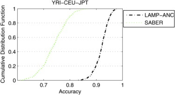
The accuracy of each of the methods varies across the population. We therefore measured the average accuracy in predicting the ancestries for each of the individuals. Figure 2 shows the cumulative distribution function of the accuracies achieved by each of the methods across the set of 500 individuals. As can be seen from the figure, the improvement of LAMP compared to STRUCTURE and SABER is quite significant. For the YRI-CEU dataset, when measuring the percentage of individuals that are predicted with an accuracy of at least 90%, LAMP achieves 90%, whereas SABER and STRUCTURE achieve less than 10%. In general, the accuracy in the predictions that STRUCTURE makes has a higher variance than the predictions made by SABER and LAMP. On the CEU-JPT dataset, LAMP is more accurate than SABER. On the JPT-CHB dataset, SABER performs considerably better than LAMP; this is probably due to the fact that the ancestral populations, which are given to SABER but not to LAMP, are too similar to distinguish within a window; because LAMP-ANC uses the allele frequencies of the ancestral individuals as input while still inferring ancestries over entire windows, it is more accurate than SABER.

Figure 2.

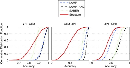
Accuracy of Ancestral Inference in Admixed Populations

Comparison of the accuracies of LAMP, LAMP-ANC, SABER, and STRUCTURE on three admixed populations—YRI-CEU (left), CEU-JPT (middle), and JPT-CHB (right). The cumulative distribution function (CDF) is obtained from the accuracy of ancestry predictions for each individual. Note that the scales differ across the plots. CDFs that are to the right side correspond to higher accuracy. The graph on the left, for instance, shows that LAMP achieves an accuracy of at least 92% on 90% of the individuals. LAMP achieves an improved accuracy over SABER and STRUCTURE in the YRI-CEU and CEU-JPT populations while performing worse on the JPT-CHB population. LAMP-ANC performs consistently well on all three populations. Also notice the decrease in accuracy across all methods as we move from left to right as the ancestral populations become more similar.

Table 1 also shows that LAMP achieves a gain in running time of at least two orders of magnitude. We found that on a single computer, LAMP and LAMP-ANC take less than 30 s to run on a 4000 SNP block and less than 7 min to run on the entire set of 38,864 SNPs.

These experiments suggest that LAMP is especially useful when the ancestral populations are sufficiently different from each other (e.g., CEU and YRI). In those cases, it is actually not essential to genotype the ancestral individuals because we observe that LAMP-ANC and LAMP achieve similar accuracy levels. When the populations are closer (e.g., CHB-JPT), even for a modest number of generations of mixing (in our case, seven generations), none of the methods performs well, even when the ancestral populations are given.

Inferring Individual Admixture

Current studies often use the individual admixture of each individual across the genome to correct for population stratification.^17,28–30 The individual admixture of an individual is defined by the proportion of ancestors of the individual from each of the ancestral populations. For instance, for an individual with a mother from CEU and a father from YRI, the individual admixture would be 50% YRI and 50% CEU.

Even though LAMP is designed to estimate the locus-specific ancestry, we can use it to find the individual admixture. We compare the estimates of the individual admixture obtained from LAMP with those from STRUCTURE. We used the YRI-CEU dataset with g = 7 and α = 0.20. We picked 4318 equally spaced SNPs from chromosome 1. This roughly matches the number of SNPs required to distinguish nonadmixed individuals from even very closely related subpopulations.³¹ We ran STRUCTURE on this set of SNPs with 10,000 burn-in iterations and 50,000 iterations with the NOLINKAGE model and the NOADMIX mode option set to 0. We ran LAMP on the entire chromosome and then calculated the locus-specific ancestry of each individual by averaging the ancestries predicted across the same set of 4318 SNPs given to STRUCTURE. As shown by Figure 3, LAMP consistently achieves considerably better estimates for the individual admixture. In particular, the average error rate for LAMP is 2.1%, whereas the average error rate for STRUCTURE is 5.4%. The difference in the performance between the methods is statistically significant (Wilcoxon signed rank test p value of 9.9 × 10⁻⁵¹). This experiment suggests that because LAMP is more than 600 times faster than STRUCTURE (see Table 1), it would be better to use LAMP across the entire genome to infer the individual admixture than to use STRUCTURE across a smaller set of ancestry-informative markers (AIMs). We also inferred the individual admixture by using the LINKAGE model in STRUCTURE but found that this gave a significantly higher average error rate of 9.0%.

Figure 3.

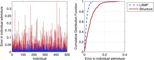
Comparison of the Accuracy of Methods for Predicting Individual Admixture

The left panel shows the errors in the individual ancestries for each of the 500 YRI-CEU individuals. The right panel shows errors in the left panel plotted as a cumulative distribution function. The top-left region of the curve corresponds to higher accuracy. LAMP predicts the individual admixture with an error of less than 3% in 80% of the cases.

Another method for the inference of the individual admixture is EIGENSTRAT. We ran EIGENSTRAT on the SNPs used above and chose the largest eigenvector. We obtained the ancestries of the individuals by scaling the entries of the eigenvector to the interval [0, 1]. We found this procedure to result in individual admixtures with an average error rate of 13.4%. When we included ten ancestral individuals each from the HapMap YRI and CEU populations, the average error was reduced to 4.1% (Wilcoxon signed rank test p value of 1.3 × 10⁻⁸³). The use of all 38,864 SNPs decreased the average error to 11.1% and 3.6%, respectively.

LAMP's Performance across Three Admixed Populations

When more than two populations are mixed, de novo inference of the locus-specific ancestry is a more challenging task. We therefore compared LAMP-ANC, which uses the genotypes from the ancestral populations, to SABER, on a dataset generated by the mixing of three populations (YRI, CEU, and JPT). We mixed these populations in the ratio 0.4:0.4:0.2 for seven generations. Figure 4 shows the ancestry estimates of LAMP-ANC for one of the individuals. LAMP-ANC accurately infers the ancestry over most of the chromosome, and it is clear that qualitatively the estimates are very close to the true ancestry. To give a more quantitative measure for the accuracy of LAMP-ANC, we calculated the cumulative distribution function of the accuracies for each individual of LAMP-ANC and of SABER (see Figure 5). Evidently, LAMP-ANC achieves a significantly better accuracy than SABER across the population (average accuracies of 92% and 74%, respectively).

Figure 4.

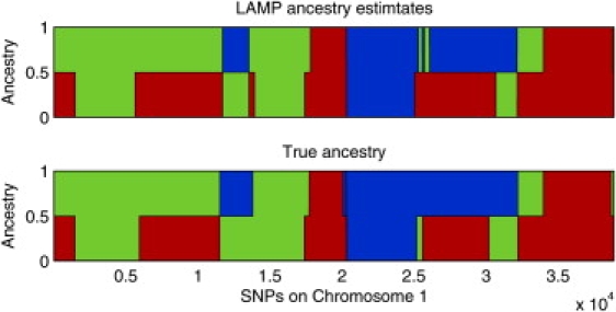
Ancestry Estimates for a Mixed-Ancestry Individual

Ancestry estimates for an individual in an admixture of YRI-CEU-JPT in the ratio 0.4, 0.4, 0.2. The top panel shows the LAMP ancestry estimates and the bottom panel the true ancestries. Red, green, and blue represent YRI, CEU, and JPT, respectively.

Figure 5.

Cumulative Distribution Function of the Accuracy Achieved per Individual

The methods compared are LAMP-ANC and SABER for the YRI-CEU-JPT admixture. LAMP achieves an accuracy of at least 80% on all the individuals.

Empirical Robustness of LAMP

The performance of LAMP clearly depends on the nature of the data, on the number of generations g, and on α. We varied g for a simulated YRI-CEU admixed population with the fraction of CEU α = 0.20. As shown in Figure 6, even when g is as large as 20, LAMP reaches an accuracy of 88%, and LAMP-ANC reaches an accuracy of 93%. For more realistic values of g, (i.e., g < 10) the accuracy of LAMP is above 93%.

Figure 6.

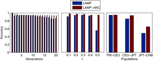
The Effects of Admixing Parameters on Accuracy

Accuracy of LAMP and LAMP-ANC with varying number of generations g, fraction of admixture α, and populations. In each figure, inferring the ancestries becomes increasingly harder as we move from left to right. The difference in the accuracies between LAMP and LAMP-ANC shows the advantage conferred by a knowledge of the ancestral allele frequencies.

To measure the effect of α on the performance of LAMP, we measured the performance for simulated data with g = 7 for different values of α (see Figure 6). We observe that LAMP performs well for values of α of up to 0.40 with its accuracy remaining above 90%, and its performance drops sharply to a little above 50% accuracy for α = 0.5.

Finally, we measured the effect of the distance between the ancestral populations by comparing the accuracy of LAMP across the YRI-CEU, CEU-JPT, and the JPT-CHB datasets. As shown in Table 1 (see also Figure 6), LAMP is quite accurate on the CEU-JPT and the YRI-CEU datasets, but its performance is quite poor on the JPT-CHB dataset. In such a situation, the availability of allele frequencies is essential for accurate inference, because we observe that LAMP-ANC maintains an accuracy of around 70%.

Robustness to Parameter Settings

Because LAMP requires as an input the values of α and g, verification that inaccurate estimates of these parameters do not affect the results significantly is important. We tested LAMP by benchmarking it over the simulated YRI-CEU dataset, with true values of g = 7 and α = 0.2. We ran LAMP on this dataset with different erroneous input values of g and α. In Figure 7, we observe that if the number of generations g is mistakenly given to LAMP as four or larger, then the accuracy of LAMP is kept reasonably high, and in particular it is at least 90%. On the other hand, it seems that if the input α is very different from the true α, LAMP can perform quite poorly. For instance, when the input α is set to 0.4 instead of 0.2, the accuracy level is about 85%. However, because α is a single parameter across all individuals, standard methods such as STRUCTURE¹² give reasonable accuracy for α (e.g., the estimates for the YRI-CEU dataset are between 0.17 and 0.24 across ten runs), we can safely assume that the error in the prior estimate of α is within a factor of 0.5, in which case LAMP maintains a very good performance.

Figure 7.

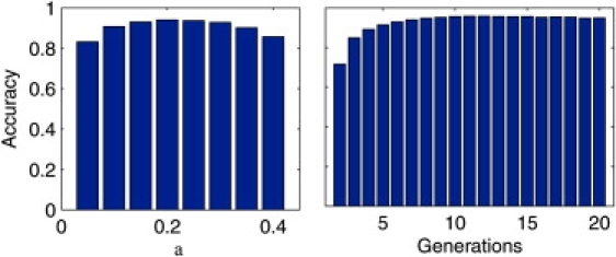
Robustness of LAMP Estimates to Uncertainty in the Parameters

Robustness of LAMP estimates to uncertainty in the parameters—g and α. The accuracy of LAMP has been shown on the YRI-CEU dataset for different values of g and α with true values of g = 7 and α = 0.20.

The model used in LAMP requires the SNPs to be independent. To ensure this, we discard SNPs with r² above a threshold. We empirically chose a threshold of 0.10 for r² so that we retain a majority of the SNPs. However, as shown in Figure 8, the accuracy of LAMP does not change much even when this threshold is raised so that the SNPs retained are no longer independent. The accuracy begins to decrease only at stringent thresholds below 0.005 because of the algorithm's tendency to discard informative SNPs. We also examined the impact of the sample size on the ancestry estimates. Although an increase in sample size might lead to SNPs being significantly linked even when the mutual r² is small, for practical purposes, such SNPs are essentially uncorrelated. Thus, LAMP is also robust to the sample size, as shown in Figure 8.

Figure 8.

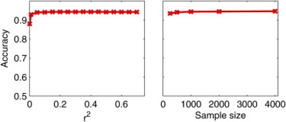
Robustness of LAMP Estimates to Sample Size and to the Choice of the Correlation-Coefficient Threshold

Robustness of LAMP estimates to the r² threshold used to discard SNPs and the sample size. The accuracy of LAMP has been shown on the YRI-CEU dataset for different values of g and α with true values of g = 7 and α = 0.20.

Finally, we measured the effect of the method used to simulate the data on the different algorithms. To achieve this, we amplified the HapMap haplotypes for YRI and CEU populations by using the model of Li and Stephens.³² Briefly, the Li and Stephens model generates additional haplotypes based on the ones already observed. The newly generated haplotypes are composed from previous ones, assuming mutation and recombination. The recombination rate in this model depends on the number of observed haplotypes, such that the rate is higher when less haplotypes are observed. This reduces the recurrent sampling of haplotypes and, as was shown by Li and Stephens, mimics more accurately the generation of haplotypes. This resulted in a set of 10,000 ancestral individuals; this set then underwent admixture with g = 7 and α = 0.20, as described earlier. On this new dataset, the accuracies obtained by LAMP, LAMP-ANC, and SABER were 94.72%, 94.70%, and 89.09%, respectively. The accuracies are close to the accuracies obtained on the YRI-CEU dataset described in Table 1.

Because the ancestral allele frequencies used in LAMP-ANC were estimated from the same data that were used for the generation of the admixed datasets, there is a potential risk of over fitting. To make sure that this is not the case, we partitioned the fouding YRI and CEU populations into two equal-sized sets. We chose one of the two sets from each population to generate a YRI-CEU dataset with parameters g = 7 and α = 0.20. Ancestral allele frequencies were estimated from the other set. The accuracy of LAMP-ANC in this setting was 94.06%, which is very close to the previous estimates obtained. Running the same procedure on the amplified datasets gave an accuracy of 94.44%, and thus we conclude that the results were not due to over fitting.

Discussion

We have presented a new method, LAMP, for de novo estimation of locus-specific ancestry in recently admixed populations. Unlike previous methods for locus-specific ancestry (e.g., SABER), LAMP does not use any information about the ancestral populations (i.e., it estimates the ancestries de novo). We show that LAMP is analytically justified and that it achieves significant improvements over existing methods both in terms of accuracy of prediction and speed. In particular, LAMP can easily be applied to whole-genome datasets, and the resulting locus-specific ancestries can be estimated within a few hours.

De novo estimation of the locus-specific ancestries is sometimes infeasible, especially when the ancestral populations are very close to each other (e.g., CHB and JPT). We therefore extended LAMP to a method called LAMP-ANC, which uses additional genotypes from the ancestral populations as priors. This approach has been shown to be useful before by methods such as SABER.

When compared to previous methods, LAMP is shown to achieve significantly better accuracy than other methods (SABER and STRUCTURE). The increase in accuracy might be crucial when one is trying to correct for population stratification in studies that involve recently admixed populations, as well as in studies that are based on admixed mapping. Furthermore, improved accuracy in the locus-specific ancestry estimation has potential applications in finding better signals for selection and other events across the genome.

Although LAMP relies on a knowledge of the parameters g and α, we have shown the robustness of the ancestry estimates to inaccuracies in these parameters. These parameters control the window size. As the window size is decreased, each window might contain fewer informative SNPs. On the other hand, errors in classifying individuals who have breakpoints within a window are reduced. This tradeoff is illustrated in Figure 7, where we see that the ancestry estimates are robust when g is overestimated. In practice, we would therefore recommend the use of an upper bound on g when g cannot be estimated accurately. Furthermore, g might actually be a more complex parameter—for example, if some portions of the admixed population have admixed for g₁ generations and other portions have been admixed for only g₂ generations, where g₂ is smaller than g₁. In this case, g is set to be g₁, and more accurate results are expected than if the whole population has admixed for exactly g1 generation.

The fact that the LAMP algorithm performs better on the unbalanced case (α << 0.5) than on the balanced case seems counterintuitive at first. The reason for this phenomenon is the fact that a small α helps to break the symmetry. Even if all windows were perfectly clustered, the combination of the solutions of the different windows into one integrated solution is not a simple task when α = 0.5 because of symmetry. That is, after clustering the individuals in every given window, we are still left with the problem of deciding which cluster is population 1 and which one is population 2. If α < 0.5, then this decision is easier because the smaller cluster could be labeled as population 1 and the larger cluster as population 2.

Further, it is interesting to note that even though SABER models the linkage disequilibrium (LD) structure whereas LAMP does not, it appears that LAMP performs better than SABER. This could be attributed to several possible reasons. First, it might be that the LD structure only adds slightly to the information captured by the independent SNPs. Second, it might be that optimization of the model in SABER is a harder task than optimization of the model in LAMP because of the larger number of parameters, and thus SABER might potentially not converge to the global optimum of its parameter space.

A simple extension to LAMP can be used to infer the individual admixture. As we show here, the resulting estimates of the individual admixture are considerably better than the estimates achieved by STRUCTURE or EIGENSTRAT. A number of recent studies have produced panels of AIMs in admixed populations;^33–36 AIMs are SNPs that have differing frequencies in the ancestral populations. It is possible that the AIMs might be used to improve the accuracy of individual admixture prediction done by STRUCTURE or other methods, including LAMP. However, the AIMs have disadvantages because there is a risk of over fitting, and the studied population might be somewhat different than the population for which the AIMs were found. As we show here, in an era where the genotyping technology is getting cheaper, it is useful to use the entire set of genotyped SNPs in the analysis of population stratification.

There are many possible improvements to this work, and in particular it would be important to improve the current methods in the case of very similar ancestral populations, or when more than two populations are involved. Furthermore, removing the dependency of the method on the input parameters (e.g., the number of generations g, or the admixture fraction α) might be quite useful for the generation of a rigorous statistical test for admixing. Additional improvements in the running time can be achieved by the parallelization of the LAMP algorithm. This is straightforward in our case because each window could be run independent of the others, and the results for windows overlapping a SNP could be aggregated in a final step.

Appendix

Correctness of MAXVAR

In this section, we analyze the correctness of the MAXVAR algorithm. We have two populations, A₁ and A₂. We denote α = α₂ as the admixture fraction of A₂—the smaller of the two populations. The MAXVAR algorithm classifies the individuals into three types of ancestries, i.e., A₁A₁, A₁A₂, and A₂A₂. The algorithm works by first picking a specific individual termed a pivot and then clustering individuals on the basis of their similarity to the pivot. We show that when the the populations are significantly different from each other, the pivot will have an ancestry A₂A₂ with high probability. In this case, we show that one can define a similarity score S (as defined in the Material and Methods), such that the individuals who are also of ancestry A₂A₂ have positive similarity score to the pivot, whereas those with ancestry A₁A₁ have negative similarity scores in expectation. Thus, the individuals with the smallest (1 − α)²n values of the similarity score are assigned an ancestry of A₁A₁, the largest α²n values are assigned an ancestry of A₂A₂, and the rest are assigned A₁A₂.

Let $p_{A_1{A}_1},p_{A_1{A}_2},\text{and}{p}_{A_2{A}_2}$ be the frequencies of individuals of the three types in the population. We assume that $p_{A_1{A}_1}={(1-\alpha )}^2$, $p_{A_2{A}_2}={\alpha }^2$, and $p_{A_1{A}_2}=2\alpha (1-\alpha )$. Let p_k and q_k be the minor allele frequencies of population A₁ and A₂, respectively, in position k. Furthermore, we assume that the values of μ_k and σ_k (as defined in the Material and Methods) are constants and that μ_k = 2(1 − α)p_k + 2αq_k, ${\sigma }_k^2=2{(1-\alpha )}^2{p}_k(1-p_k)+2\alpha (1-\alpha )[p_k(1-p_k)+q_k(1-q_k)]+2{\alpha }^2{q}_k(1-q_k).$ Note that by simplifying the above, one gets that ${\sigma }_k^2=2(1-\alpha )p_k(1-p_k)+2\alpha q_k(1-q_k)$, and therefore it is of the same order of magnitude as μ_k for common SNPs. If the number of individuals is large enough, the variance is quite low, and therefore this is not a restrictive assumption. We define the distance between the two populations as $W=\sum _k\frac{{\left(p_k-q_k\right)}^2}{{\sigma }_k^2}$. Under these assumptions, it is easy to see that if aa, ab, and bb are three given individuals with ancestry A₁A₁, A₁A₂, and A₂A₂, respectively, in the window, then the expected similarity score S between pairs of individuals is

$$\begin{array}{c}E\left[S(aa,a{a}^{\prime })\right]=4{\mathit{\alpha }}^{2}W,E\left[S(aa,ab)\right]=-2(1-2\mathit{\alpha })\mathit{\alpha }W,\\ E\left[S(aa,bb)\right]=-4(1-\mathit{\alpha })\mathit{\alpha }W,E\left[S(ab,a{b}^{\prime })\right]={(1-2\mathit{\alpha })}^{2}W,\\ E\left[S(ab,bb)\right]=2(1-2\mathit{\alpha })(1-\mathit{\alpha })W,E\left[S(bb,b{b}^{\prime })\right]=4{(1-\mathit{\alpha })}^{2}W,\end{array}$$ (9)

where aa′, ab′, and bb′ are individuals with ancestries A₁A₁, A₁A₂, and A₂A₂, but they are different individuals than aa, ab, and bb. From this, it is easy to verify that the sum of squares of expectations over all individuals that are different from aa, ab, and bb can be approximated as:

$$\begin{array}{c}\sum _{i:i\ne aa}{\left[E\left[S(i,aa)\right]\right]}^2\approx 8{\alpha }^3(1-\alpha )W^{2}n\\ \sum _{i:i\ne ab}{\left[E\left[S(i,ab)\right]\right]}^2\approx 2\alpha (1-\alpha ){(1-2\alpha )}^2{W}^{2}n\\ \sum _{i:i\ne bb}{\left[E\left[S(i,bb)\right]\right]}^2\approx 8{(1-\alpha )}^3\alpha W^{2}n\end{array}.$$ (10)

The only reason for the approximation is that the number of individuals with ancestry A₂A₂ that are different from bb is (1 − α)²n − 1, whereas we consider it as (1 − α)²n. This approximation is not restrictive when the number of individuals is reasonably large.

Similarly, it is easy to verify that if m is the number of SNPs, then the following holds:

$$\begin{array}{c}\sum _{i:i\ne aa}Var\left[S(i,aa)\right]<n\sum _k\frac{4{\mu }_k^2(p_k^2+\alpha (p_k-q_k)(1-{\mu }_k))}{{\sigma }_k^4}=O\left(nm\right)\\ \sum _{i:i\ne ab}Var\left[S(i,ab)\right]<n\sum _k\frac{4{\mu }_k^2(p_k{q}_k+(2\alpha -1)(p_k-q_k)(1-{\mu }_k))}{{\sigma }_k^4}=O\left(nm\right)\\ \sum _{i:i\ne bb}Var\left[S(i,bb)\right]<n\sum _k\frac{4{\mu }_k^2(q_k^2-(1-\alpha )(p_k-q_k)(1-{\mu }_k))}{{\sigma }_k^4}=O\left(nm\right)\end{array}.$$

The bounds O(m) follow from the fact that ${\mu }_k=\Theta \left({\sigma }_k^2\right)$ for every common SNP with minor allele frequency bounded away from zero. Therefore, if we assume that $W>>\sqrt{m}$ (i.e., the populations are distant from each other), we get that for every individual x, $\sum _{i:i\ne x}E{\left[S(i,aa)\right]}^2>>\sum _{i:i\ne x}Var\left[S(i,aa)\right]$. On the other hand,

$$\sum _{i:i\ne x}E\left[{\left(S(i,x)\right)}^2\right]=\sum _{i:i\ne x}E{\left[S(i,x)\right]}^2+\sum _{i:i\ne x}Var\left[S(i,x)\right]\approx \sum _{i:i\ne x}E{\left[S(i,x)\right]}^2.$$

From Equation 10, we conclude that the expectation of the square of distances of the population from an individual from A₂A₂ is larger than from and individual from A₁A₂, or A₁A₁. If the number of individuals is large enough, the distribution is concentrated around the mean, and thus we expect an A₂A₂ individual to be chosen as the pivot. In that case, by Equation 9, the ordering of the individuals according to their similarity to the pivot should give the correct clustering with a fraction of errors exponentially small in W.

Accuracy of the Window Length and the Majority Vote

For a given window, the analysis in the Choosing the Window Length section shows that the expected fraction of individuals with no breakpoints is 1 − γ. Here, we strengthen this analysis under the assumption that the errors in the predictions of the different windows are independent.

It is easy to see that the expected fraction of individuals with two or more breakpoints in a window is smaller than γ². For a given individual with a breakpoint in position i, we denote the ancestry by $(A_{s_1},A_{s_2},i,A_{s_3})$, where $A_{s_1}$ is the ancestry of the nonrecombinant chromosome and $A_{s_2}$ and $A_{s_3}$ are the ancestries of the recombinant chromosome. We assume that the probability to classify such an individual as $A_{s_1}{A}_{s_2}$ is $\frac{i}{l}$ and the probability to classify it as $A_{s_1}{A}_{s_3}$ is $1-\frac{i}{l}$. There are l windows that overlap with any SNP. Consider a SNP that is a distance d away from a breakpoint. Let X be the number of times that the SNP is incorrectly classified as $A_{s_1}{A}_{s_3}$. Clearly,

$$E\left[X\right]=\sum _{i=1}^{l-d}\frac{i}{l}\approx \frac{{(l-d)}^2}{2l}.$$

With a Chernoff bound,³⁷ the probability of incorrectly classifying this SNP after the majority vote is

$$\mathrm{Pr}(X>\frac{l}{2})=\mathrm{Pr}(X>{(1+\frac{d}{l-d})}^{2}E\left[X\right])<e^{-\frac{{\left(\frac{d}{l-d}(2+\frac{d}{l-d})\right)}^{2}E\left[X\right]}{2}}=e^{-\frac{{(d(2+\frac{d}{l-d}))}^2}{4l}}<e^{-\frac{d^2}{l}}.$$

In the case that there are no other breakpoints within distance l from the breakpoint considered, the expected number of errors around the breakpoint for the individual is bounded by

$${\int }_0^l{e}^{\frac{-x^2}{l}}dx={\int }_0^{\sqrt{2l}}{e}^{\frac{-x^2}{2}}\sqrt{l/2}dx\le \sqrt{l/2}\sqrt{2\pi }=\sqrt{l/\pi }.$$

If there are breakpoints within distance l of each other, we take the worst-case assumption that all windows containing the two breakpoints make erroneous predictions over their entire length l. Because the expected fraction of breakpoints in an individual is $\frac{\gamma }{l}$ and the expected fraction of pairs of breakpoints that are of distance smaller than l is at most $\frac{{\gamma }^2}{l}$, we can bound the expected fraction of errors as $\frac{\gamma }{\sqrt{\pi l}}+{\gamma }^2=4\sum _{i<j}{\mathit{\alpha }}_i{\mathit{\alpha }}_j(g-1)r(\sqrt{\frac{l}{\pi }}+4\left(\sum _{i<j}{\mathit{\alpha }}_i{\mathit{\alpha }}_j\right)(g-1)r{l}^2)$. On the basis of this analysis, a sufficient condition to achieve a desired error rate of ɛ is to have

$$l<\min \left\{\frac{1}{4(g-1)r\sum _{i<j}{\mathit{\alpha }}_i{\mathit{\alpha }}_j}\sqrt{\frac{\varepsilon }{2}},\frac{\pi {\varepsilon }^2}{{(4(g-1)r\sum _{i<j}{\mathit{\alpha }}_i{\mathit{\alpha }}_j)}^2}\right\}.$$

Estimate of Window Length

The window length derived in Equation 8 bounds the classification errors within each window to a desired error rate ɛ. Because all SNPs within a window are assigned the same ancestry, any algorithm that is used within this window will incur some errors in the presence of breakpoints. Hence, the window length was calculated under the assumption that the classification algorithm within the window was the most accurate possible, i.e., any errors in the classification were only a result of breakpoints within a window. Here, we empirically show that for the window lengths computed with Equation 8, the average classification error for a most accurate classification is bounded by the error rate ɛ, which is set to 0.10.

Within each window, the most accurate ancestry assignment is inferred with the assumption that the true ancestries are known. The most accurate assignment consists of assigning to an individual the ancestry found in a majority of the SNPs in that window. Thus, an individual who has no breakpoints is always correctly classified, whereas an individual with a breakpoint at position $i<\lceil \frac{l}{2}\rceil$ in a window of length l and ancestries $A_{s_1}$ and $A_{s_2}$ on either side of the breakpoint will have errors in positions {1,…,i}. The error rate for a window is the fraction of positions that are incorrectly classified in the window.

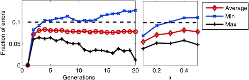
We computed the average of these errors in overlapping windows that span chromosome 1 of the YRI-CEU dataset for different values of g and α. We see in Figure 9 that the average error is below ɛ. However, the variance of the estimates (indicated by the minimum and the maximum fraction of errors) increases with larger g or with $\mathit{\alpha }\to 0.5$. The window-size estimates seem to provide a good bound on the average fraction of errors due to breakpoints.

Figure 9.

Empirical Validation of the Window-Length Estimates

The window length is estimated in the Material and Methods (Choosing the Window Length). These estimates are based on a parameter ɛ, which represents the average desired fraction of errors incurred by the most accurate classification algorithm that can only return one of A₁A₁, A₁A₂, A₂A₂ for the entire window. The figure presents the actual average error rates for different values of g and α, run on the CEU-YRI dataset, with ɛ = 0.1. Evidently, the actual average error rate falls within the desired error bound. The maximum and the minimum fraction of errors in a window are also shown.

Practical Issues in Implementing LAMP

In this section, we describe some of the issues that we faced while implemeting LAMP. One of the issues that we needed to address was how to determine the degree of overlap between adjacent windows. An extreme degree of overlap would require adjacent windows to differ in a single SNP. In practice, we found that a smaller degree of overlap, where consecutive windows overlapped in a fraction c = 80% of their length, did not significantly change the accuracy while resulting in faster running times. The overlap between adjacent windows can be exploited to further improve the running time. Although using the MAXVAR algorithm to obtain an initial classification, each window requires a computation of the similarity score between all pairs of individuals. The similarity score is computed with an inner product of the normalized genotypes, as described in the Initializing the Clusters section. Instead of computing these similarity scores over entire windows of length l, we can compute these scores over chromosomes of length (1 − c)l. The similarity score in a new window can then be computed from that of the previous window by adjusting for the nonoverlapping regions.

As we mentioned at the end of the Choosing the Window Length section, the window length calculation should take into account the distance between the two populations. This is feasible when the ancestral genotypes are known. In this scenario, the accuracy of the classification for a given window length can be obtained by running LAMP-ANC on the ancestral genotypes. With an increase in the window length, this accuracy is exptected to increase. On the other hand, the errors due to breakpoints, as given in Equation 8, increase with window length. We can then search for the window length that maximizes the product of the fraction of individuals who do not have breakpoints and the fraction of these individuals who are accurately classified. For populations that are well separated, such as YRI-CEU and CEU-JPT, we find that the number of SNPs needed to accurately classify a nonadmixed individual is much smaller than the length of the window obtained from Equation 8, so that it suffices to simply set the window length to the latter estimate.

Web Resources

The URLs for data presented herein are as follows:

• LAMP program, http://lamp.icsi.berkeley.edu/lamp/

• Hapmap project, http://www.hapmap.org

• Affymetrix GeneChip Human Mapping 500K Array Set, http://www.affymetrix.com/products/arrays/specific/500k.affx

References

- 1.Bonnen P.E., Pe'er I., Plenge R.M., Salit J., Lowe J.K., Shapero M.H., Lifton R.P., Breslow J.L., Daly M.J., Reich D.E. Evaluating potential for whole-genome studies in Kosrae, an isolated population in Micronesia. Nat. Genet. 2006;38:214–217. doi: 10.1038/ng1712. [DOI] [PubMed] [Google Scholar]
- 2.Price A.L., Patterson N.J., Plenge R.M., Weinblatt M.E., Shadick N.A., Reich D. Principal components analysis corrects for stratification in genome-wide association studies. Nat. Genet. 2006;38:904–909. doi: 10.1038/ng1847. [DOI] [PubMed] [Google Scholar]
- 3.Freedman M.L., Reich D., Penney K.L., McDonald G.J., Mignault A.A., Patterson N., Gabriel S.B., Topol E.J., Smoller J.W., Pato C.N. Assessing the impact of population stratification on genetic association studies. Nat. Genet. 2004;36:388–393. doi: 10.1038/ng1333. [DOI] [PubMed] [Google Scholar]
- 4.Clayton D.G., Walker N.M., Smyth D.J., Pask R., Cooper J.D., Maier L.M., Smink L.J., Lam A.C., Ovington N.R., Stevens H.E. Population structure, differential bias and genomic control in a large-scale, case-control association study. Nat. Genet. 2005;37:1243–1246. doi: 10.1038/ng1653. [DOI] [PubMed] [Google Scholar]
- 5.Lander E.S., Schork N.J. Genetic dissection of complex traits. Science. 1994;265:2037–2048. doi: 10.1126/science.8091226. [DOI] [PubMed] [Google Scholar]
- 6.Helgason A., Yngvadóttir B., Hrafnkelsson B., Gulcher J., Stefánsson K. An Icelandic example of the impact of population structure on association studies. Nat. Genet. 2005;37:90–95. doi: 10.1038/ng1492. [DOI] [PubMed] [Google Scholar]
- 7.Campbell C.D., Ogburn E.L., Lunetta K.L., Lyon H.N., Freedman M.L., Groop L.C., Altshuler D., Ardlie K.G., Hirschhorn J.N. Demonstrating stratification in a European American population. Nat. Genet. 2005;37:868–872. doi: 10.1038/ng1607. [DOI] [PubMed] [Google Scholar]
- 8.Hirschhorn J.N., Daly M.J. Genome-wide association studies for common diseases and complex traits. Nat. Rev. Genet. 2005;6:95–108. doi: 10.1038/nrg1521. [DOI] [PubMed] [Google Scholar]
- 9.Lohmueller K.E., Pearce C.L., Pike M., Lander E.S., Hirschhorn J.N. Meta-analysis of genetic association studies supports a contribution of common variants to susceptibility to common disease. Nat. Genet. 2003;33:177–182. doi: 10.1038/ng1071. [DOI] [PubMed] [Google Scholar]
- 10.Marchini J., Cardon L.R., Phillips M.S., Donnelly P. The effects of human population structure on large genetic association studies. Nat. Genet. 2004;36:512–517. doi: 10.1038/ng1337. [DOI] [PubMed] [Google Scholar]
- 11.Devlin B., Roeder K. Genomic control for association studies. Biometrics. 1999;55:997–1004. doi: 10.1111/j.0006-341x.1999.00997.x. [DOI] [PubMed] [Google Scholar]
- 12.Pritchard J.K., Stephens M., Donnelly P. Inference of population structure using multilocus genotype data. Genetics. 2000;155:945–959. doi: 10.1093/genetics/155.2.945. [DOI] [PMC free article] [PubMed] [Google Scholar]
- 13.Setakis E., Stirnadel H., Balding D.J. Logistic regression protects against population structure in genetic association studies. Genome Res. 2006;16:290–296. doi: 10.1101/gr.4346306. [DOI] [PMC free article] [PubMed] [Google Scholar]
- 14.Reich D., Patterson N., De Jager P.L., Mcdonald G.J., Waliszewska A., Tandon A., Lincoln R.R., Deloa C., Fruhan S.A., Cabre P. A whole-genome admixture scan finds a candidate locus for multiple sclerosis susceptibility. Nat. Genet. 2005;37:1113–1118. doi: 10.1038/ng1646. [DOI] [PubMed] [Google Scholar]
- 15.Zhu X., Luke A., Cooper R.S., Quertermous T., Hanis C., Mosley T., Gu C.C., Tang H., Rao D.C., Risch N. Admixture mapping for hypertension loci with genome-scan markers. Nat. Genet. 2005;37:177–181. doi: 10.1038/ng1510. [DOI] [PubMed] [Google Scholar]
- 16.Patterson N., Hattangadi N., Lane B., Lohmueller K.E., Hafler D.A., Oksenberg J.R., Hauser S.L., Smith M.W., O'Brien S.J., Altshuler D. Methods for high-density admixture mapping of disease genes. Am. J. Hum. Genet. 2004;74:979–1000. doi: 10.1086/420871. [DOI] [PMC free article] [PubMed] [Google Scholar]
- 17.Falush D., Stephens M., Pritchard J.K. Inference of population structure using multilocus genotype data: Linked loci and correlated allele frequencies. Genetics. 2003;164:1567–1587. doi: 10.1093/genetics/164.4.1567. [DOI] [PMC free article] [PubMed] [Google Scholar]
- 18.Hoggart C.J., Shriver M.D., Kittles R.A., Clayton D.G., McKeigue P.M. Design and analysis of admixture mapping studies. Am. J. Hum. Genet. 2004;74:965–978. doi: 10.1086/420855. [DOI] [PMC free article] [PubMed] [Google Scholar]
- 19.Tang H., Coram M., Wang P., Zhu X., Risch N. Reconstructing genetic ancestry blocks in admixed individuals. Am. J. Hum. Genet. 2006;79:1–12. doi: 10.1086/504302. [DOI] [PMC free article] [PubMed] [Google Scholar]
- 20.Rabiner L. A tutorial on hmm and selected applications in speech recognition. Proc. IEEE. 1989;77:257–286. [Google Scholar]
- 21.Haldane J.B.S. The combination of linkage values and the calculation of distance between the loci of linked factors. J. Genet. 1919;8:299–309. [Google Scholar]
- 22.Besag J. On the statistical analysis of dirty pictures. Journal of the Royal Statistical Society Series B (Methodological) 1986;48:259–302. [Google Scholar]
- 23.Myers S., Bottolo L., Freeman C., McVean G., Donnelly P. A fine-scale map of recombination rates and hotspots across the human genome. Science. 2005;310:321–324. doi: 10.1126/science.1117196. [DOI] [PubMed] [Google Scholar]
- 24.Nachman M.W., Crowell S.L. Estimate of the mutation rate per nucleotide in humans. Genetics. 2000;156:297–304. doi: 10.1093/genetics/156.1.297. [DOI] [PMC free article] [PubMed] [Google Scholar]
- 25.Tian C., Hinds D.A., Shigeta R., Kittles R., Ballinger D.G., Seldin M.F. A genomewide single-nucleotide-polymorphism panel with high ancestry information for African American admixture mapping. Am. J. Hum. Genet. 2006;79:640–649. doi: 10.1086/507954. [DOI] [PMC free article] [PubMed] [Google Scholar]
- 26.Parra E.J., Marcini A., Akey J., Martinson J., Batzer M.A., Cooper R., Forrester T., Allison D.B., Deka R., Ferrell R.E. Estimating african american admixture proportions by use of population-specific alleles. Am. J. Hum. Genet. 1998;63:1839–1851. doi: 10.1086/302148. [DOI] [PMC free article] [PubMed] [Google Scholar]
- 27.Collins-Schramm H.E., Chima B., Operario D.J., Criswell L.A., Seldin M.F. Markers informative for ancestry demonstrate consistent megabase-length linkage disequilibrium in the african american population. Hum. Genet. 2003;113:211–219. doi: 10.1007/s00439-003-0961-1. [DOI] [PubMed] [Google Scholar]
- 28.Shriver M.D., Smith M.W., Jin L., Marcini A., Akey J.M., Deka R., Ferrell R.E. Ethnic-affiliation estimation by use of population-specific dna markers. Am. J. Hum. Genet. 1997;60:957–964. [PMC free article] [PubMed] [Google Scholar]
- 29.Ziv E., Burchard E.G. Human population structure and genetic association studies. Pharmacogenomics. 2003;4:431–441. doi: 10.1517/phgs.4.4.431.22758. [DOI] [PubMed] [Google Scholar]
- 30.Hanis C.L., Chakraborty R., Ferrell R.E., Schull W.J. Individual admixture estimates: Disease associations and individual risk of diabetes and gallbladder disease among mexican-americans in starr county, texas. Am. J. Phys. Anthropol. 1986;70:433–441. doi: 10.1002/ajpa.1330700404. [DOI] [PubMed] [Google Scholar]
- 31.Sridhar, S., Rao, S., and Halperin, E. (2007). An efficient and accurate graph-based method to detect population substructure. Proceedings of Research in Computational Molecular Biology (RECOMB), pp. 503–517.
- 32.Li N., Stephens M. Modeling linkage disequilibrium and identifying recombination hotspots using single-nucleotide polymorphism data. Genetics. 2003;165:2213–2233. doi: 10.1093/genetics/165.4.2213. [DOI] [PMC free article] [PubMed] [Google Scholar]
- 33.Tian C., Hinds D.A., Shigeta R., Adler S.G., Lee A., Pahl M.V., Silva G., Belmont J.W., Hanson R.L., Knowler W.C. A genome-wide snp panel for mexican american admixture mapping. Am. J. Hum. Genet. 2007;80:1014–1023. doi: 10.1086/513522. [DOI] [PMC free article] [PubMed] [Google Scholar]
- 34.Mao X., Bigham A.W., Mei R., Gutierrez G., Weiss K.M., Brutsaert T.D., Leon-Velarde F., Moore L.G., Vargas E., McKeigue P.M. A genome-wide admixture mapping panel for hispanic/latino populations. Am. J. Hum. Genet. 2007;80:1171–1178. doi: 10.1086/518564. [DOI] [PMC free article] [PubMed] [Google Scholar]
- 35.Price A.L., Patterson N., Yu F., Cox D.R., Waliszewska A., McDonald G.J., Tandon A., Schirmer C., Neubauer J., Bedoya G. A genomewide admixture map for latino populations. Am. J. Hum. Genet. 2007;80:1024–1036. doi: 10.1086/518313. [DOI] [PMC free article] [PubMed] [Google Scholar]
- 36.Smith M.W., Patterson N., Lautenberger J.A., Truelove A.L., McDonald G.J., Waliszewska A., Kessing B.D., Malasky M.J., Scafe C., Le E. A high-density admixture map for disease gene discovery in African Americans. Am. J. Hum. Genet. 2004;74:1001–1013. doi: 10.1086/420856. [DOI] [PMC free article] [PubMed] [Google Scholar]
- 37.Chernoff H. A measure of asymptotic efficiency for tests of a hypothesis based on the sum of observations. Ann. Math. Stat. 1952;23:493–507. [Google Scholar]