Bayesian Meta-Analysis of Genetic Association Studies with Different Sets of Markers

Abstract

Robust assessment of genetic effects on quantitative traits or complex-disease risk requires synthesis of evidence from multiple studies. Frequently, studies have genotyped partially overlapping sets of SNPs within a gene or region of interest, hampering attempts to combine all the available data. By using the example of C-reactive protein (CRP) as a quantitative trait, we show how linkage disequilibrium in and around its gene facilitates use of Bayesian hierarchical models to integrate informative data from all available genetic association studies of this trait, irrespective of the SNP typed. A variable selection scheme, followed by contextualization of SNPs exhibiting independent associations within the haplotype structure of the gene, enhanced our ability to infer likely causal variants in this region with population-scale data. This strategy, based on data from a literature based systematic review and substantial new genotyping, facilitated the most comprehensive evaluation to date of the role of variants governing CRP levels, providing important information on the minimal subset of SNPs necessary for comprehensive evaluation of the likely causal relevance of elevated CRP levels for coronary-heart-disease risk by Mendelian randomization. The same method could be applied to evidence synthesis of other quantitative traits, whenever the typed SNPs vary among studies, and to assist fine mapping of causal variants.

Introduction

Genetic effects underlying complex traits and disorders are small, and their detection requires comprehensive typing of single nucleotide polymorphisms (SNPs) in large samples.^1,2 Many previous genetic association studies have been underpowered,^3,4 and even very large biobanks⁵ may not individually provide conclusive results for certain outcomes. Quantitative synthesis of evidence from available studies remains vital,^6–8 even in the era of genome-wide analyses.^9–11 However, a major obstacle is that studies of the same gene, region, or even the genome as a whole may type a different repertoire of SNPs, thereby yielding partially overlapping genotypic data. Moreover, often only single SNP summary data, for instance genotype means at each SNP, is reported.

The meta-analysis of results from each marker in isolation would exclude those studies that did not type the marker in question, with a potential loss of power; moreover, multiple single-SNP analyses are difficult to interpret. Instead, it would be useful to be able to combine data with information from all sites, adjusting any association at each site for the possible correlation with the remaining variants. One could then disentangle effects at causal sites from those at sites that are in LD with a causal variant(s) and also borrow information across studies. With focus on a quantitative trait, we develop a Bayesian hierarchical linear regression that models linear transformations of the study-specific genotype-group-specific phenotypic means and that uses pairwise LD measurements between markers to make posterior inference on adjusted effects. Information on pairwise marker LD is often provided by the individual studies as part of the results reported. Alternatively, for markers that are not considered jointly in any of the study at hand, it can often be obtained from public databases. This information is then used to specify informative priors in our Bayesian framework. Specifically, the between-marker correlations are modeled by introduction of spatially correlated random effects having a conditional autoregressive distribution (CAR).^12,13 The between-study variability is then accommodated with a random intercept term across studies.

Our approach is motivated by the meta-analysis of studies assessing the effect of variants in the C-reactive protein (CRP [MIM 123260]) gene region on plasma CRP levels. CRP is a circulating monomorphic hepatic acute-phase protein that indexes and may mediate aspects of the inflammatory response.¹⁴ Aside from acute-phase elevations, blood concentrations of CRP show similar within-individual variability to serum cholesterol, and like cholesterol, CRP has been shown to be associated with future coronary heart disease (CHD) risk in observational studies.¹⁵ However, the etiological relevance of this potentially important and highly studied link with CHD is uncertain because CRP may simply be a marker for established risk factors or for subclinical atheroma.^16,17 Common SNPs that are in the gene encoding CRP and that influence its level may help provide insight on the link because, unlike CRP itself, genotype is fixed and unaffected by subclinical disease and the naturally randomized allocation of alleles at conception balances the distribution of potential confounding factors among genotypic classes. Genetic associations are therefore less prone to biases that limit causal inference from observational studies, and genetic studies possess properties of a randomized intervention trial.^16–18 Therefore, identification of CRP-gene variants (HGNC: 2637; 1q21-q23) that influence its concentration is fundamental to evaluating the causal relevance of CRP with the principle of Mendelian randomization.¹⁹

In the absence of hepatic stores of CRP, and given its constant rate of clearance, gene transcription provides the major point of regulation.¹⁴ Transcription may be modified by regulatory SNPs because concentrations of CRP show strong concordance among monozygotic twins and family studies suggest substantial heritability.²⁰ In populations of European descent, there are 11 common SNPs with minor allele frequency >5% within 6 kb of the CRP gene, but extensive linkage disequilibrium (LD) means that four major haplotypes account for 94% of chromosomes (see Web Resources).^21,22 Individual reports evaluating associations of CRP SNPs with CRP concentration have either typed single SNPs or a subset of SNPs (sometimes tag SNPs) in this region (see Table S1 available online). However, the SNPs have varied across studies, thereby limiting the ability to pool all available data. We therefore developed a new integrative approach to evidence synthesis of genetic association studies that allows for this complexity.

Methods for combining data from genome-wide scans with nonoverlapping sets of SNPs with individual-level genotyping data have been recently proposed by Marchini et al.²³ Here, because individual-level data are not available for most of the studies on CRP, we develop a method that allows the synthesis of studies providing only summary data. Also, we are mainly concerned with the synthesis of SNP data in regions of interest for fine mapping, where the number of markers typed is small and interest is on disentangling independent effects using a variable selection scheme, for which the Marchini approach is not suitable.

Material and Methods

We first conducted a literature-based systematic review of all relevant studies (irrespective of the SNP typed). A total of 23 published data sets identified by systematic review evaluated associations of eight SNPs (rs3093059; rs2794521; rs3091244; rs1417938; rs1800947; rs1130864; rs1205; and rs3093077) in the CRP gene with CRP concentration (Figure 1). With data from SeattleSNPs, a combination of three SNPs (rs1130864; rs1205; and rs3093077) was identified as haplotype tag SNPs with the haplotype r² method in European subjects. These tag SNPs were typed in three additional population-based studies, thereby giving an aggregate of 26 studies including 32,802 subjects. No SNP was typed in every study, but there was partial overlap of SNP typing across several studies (see Appendix A and Table S1).

Figure 1.

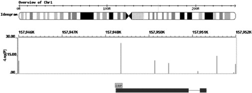
Location of the Eight CRP SNPs Typed Directly in the 26 Data Sets Included in This Study

The upper track shows chromosomal location; the middle track shows SNP location and Log(P) for the per-allele random-effect meta-analysis (from left to right, the SNPs are ordered as follows: rs3093077, rs1205, rs1130864, rs1800947, rs1417938, rs3091244, rs2794521, and rs3093059); and the lower track shows the intron/exon structure of the CRP gene.

Bayesian Hierarchical Model

We indicate with Y_i^s the continuous trait of interest for subject $i\in \{1,\dots ,n^s\}$ and study $s\in \{1,\dots ,S\}$. If all studies have genotyped individuals at all m marker locations, and these data are available for all individuals (individual patient data [IPD]), a sensible approach to pool information across studies would be the random-effect model

$${\mathbf{Y}}^s\sim \mathrm{N}({\mathbf{C}}^s\beta +1_{n^s}{\mu }_s,{\sigma }^2{\mathbf{I}}_{n^s})$$ (1)

where C^s is the n^s × (m + 1) design matrix coding for the chosen genetic model (e.g., for an additive models, 0, 1, and 2 for homozygous wild-type, heterozygous, or homozygous mutant genotypes, respectively) and the intercept term, μ_s ∼N(0, σ²_s) is a study-specific random intercept term, ${\mathbf{1}}_{n^s}$ is the n^s × 1 vector of ones, ${\mathbf{I}}_{n^s}$ is the n^s × n^s identity matrix, and $\beta =({\beta }_0,{\beta }_1,\dots ,{\beta }_m)\prime$ is the (m + 1) × 1 vector of regression coefficients of interest measuring the effect of genotype group on Y. One could then assess the relative importance of each marker by using a variable selection scheme; we use a reversible jump algorithm on the space of possible models as part of the MCMC scheme as described later in the text.^24,25

However, studies will rarely consider all m markers together; rather, m_s ≤ m will have been typed in study s corresponding to a subset L_s of columns of the complete design matrix C^s, X^s say of size n^s × (m_s + 1). Also, complete individual patient data for all studies are rarely available. Instead, we have the summary statistics reported in each study as in the case of the CRP studies. Typically, data will consist of means, variances, and numbers of individuals for each genotype groups and each marker. These are denoted by ${\overline{y}}_{gj}^s$, v_gj^s, and n_gj^s, respectively, for genotype group $g=1,\dots ,G_j$ of marker j ∈ {L_s} in study s. The notation allows for marker-specific numbers of genotype groups and thus the possibility of having a mixture of biallelic and triallelic markers, as in the application to the CRP data, or different genetic models.

Our approach uses Equation (1) as the building block but models the linear transformations T^s = X^s′Y^s as multivariate normally distributed across studies

$${\mathbf{T}}^s{\sim \text{MVN}}_{m_s}({\mathbf{X}}^{s\prime }{\mathbf{C}}^s\beta +{\mathbf{X}}^{s\prime }{\mathbf{1}}_{n^s}{\mu }_s,{\sigma }^2{\mathbf{X}}^{s\prime }{\mathbf{X}}^s)$$ (2)

where X^s′ indicates the transpose of X^s. All entries of the vector T^s can be obtained from the available data summaries. For instance, the first element corresponding to the intercept term is the overall sum of the y values, and any other entry can be obtained similarly from the genotype-group-specific phenotype means and counts ${\overline{y}}_{gj}^s,n_{gi}^s.$

However, the new design matrix W^s = X^s′C^s is only partially observed. In particular, only the dot products involving the columns of X^s with themselves or the intercept term can be derived from the observed genotype-group counts. The remaining entries are replaced by their expected values under Hardy-Weinberg equilibrium (HWE) and the known pairwise LD patterns. Specifically, indicating with w_hl, h ≠ l, a generic such entry, we first obtain an estimate of the joint bivariate genotype distribution from the known marginal allele frequencies and the pairwise measure of LD.²⁶ For example, if both markers are biallelic, this involves estimation of the 3 × 3 matrix of the genotype distribution, and this estimation is then multiplied by the study size to give expected counts. Finally, we obtained w_hl by summing the appropriate entries of the resulting matrix of expected counts multiplied by the values used to code the genotype groups in the design matrices. Notice that the vector of coefficients β retains the same interpretation and scale of the original model in Equation (1) (in the example below, additive effect of variants on log CRP plasma levels) because it is derived from a linear transformation of the variables therein.

As well as in the derivation of the new design matrix W^s, prior information of between-marker LD patterns is also incorporated in the specification of the (partially unobserved) variance-covariance matrix in Equation (2). Specifically, we partition σ²X^s′X^s into a spatially structured component and a residual, unstructured, component. We obtained the former by introducing marker-specific random effects having a zero-mean conditional autoregressive distribution

$$\mathbf{U}\sim \text{CAR}\left(\mathbf{0},{\sigma }_u^2{(\mathbf{I}-\gamma \mathbf{R})}^{-1}\mathbf{M}\right)$$ (3)

where U is a vector of size m, the number of unique markers across studies, R is a matrix of weights reflecting spatial associations between the elements of T^s, and M is a diagonal matrix.^12,27 Thus the covariance matrix in Equation (2) becomes σ²_u(I − γR)⁻¹M + σ²_ɛdiag(X′X) where we set γ ≡ 1 and (I − γR)⁻¹M ≡ (X′X − diag(X′X)), where with X′X we indicate the weighted average of the study-specific cross-products X^s′X^s with weights given by the number of subjects in each study. The latter equivalence then reflects our prior information on pairwise LD, as the off-diagonal elements of the matrix X^s′X^s′ are replaced by their expected values given the LD patterns.

Conditional on the study and marker-specific random effects μ_s and U_j, the elements of T^s are independent and we can rewrite Equation (2) as

$$T_j^s|{\mu }_s,U_j\sim \mathrm{N}\left({\mathbf{W}}_{j,\cdot }\beta +{\sum _{i=1}^{n_s}{x}^s}_{i,j}{\mu }_s+U_j,{\sigma }_{\epsilon }^2\text{diag}{\left({\mathbf{X}}^{s\prime }{\mathbf{X}}^s\right)}_{j,j}\right)$$ (4)

$$j\in \left\{L_s\right\}.$$

We further assume that the marker and study-specific pooled variances

$$v_{.j}^s=\frac{\sum _g(n_{gj}-1)v_{gj}^s}{\sum _g(n_{gj}-1)}$$

have a scaled chi-square distribution

$$v_{.j}^s=\frac{{\sigma }_{\epsilon }^2}{\sum _g{n}_{g{j}^s}-G_j}{\chi }_{\sum _g{n}_{g{j}^s}-G_j}.$$

Albeit an approximation, this assumption is likely to hold when the individual SNP associations are modest, as it is reasonable to expect in this setting. Also, by modeling the observed variances, we are able to impute any missing values from their full conditional distribution as part of the MCMC scheme.

The hierarchical specification is completed by assuming a distribution for the between-studies random effects μ_s. In order to accommodate outliers and heavy tails, we assume the mixture of normals

$${\mu }_s\sim \pi \mathrm{N}({\alpha }_1,{\sigma }_{\mu }^2)+(1-\pi )\mathrm{N}({\alpha }_2,{\sigma }_{\mu }^2).$$ (5)

with ${\alpha }_2=-\pi {\alpha }_1/(1-\pi ).$²⁸

To select important marker-phenotype associations, we use a reversible jump algorithm on the space of models in the MCMC scheme.^24,25 In brief, denoting with k the number of SNP currently included in a model, we made a proposal to change the current model by adding a marker, deleting a marker, or swapping a marker currently in the model with one from the remaining SNPs. The new model is accepted with probability proportional to its likelihood. Conditional on the accepted model, new values for the appropriate subset of parameters in β are then sampled from their full conditional distribution. By monitoring the different models visited, we readily obtained posterior model probabilities. The algorithm is not guaranteed to visit all possible models, but in many cases, if the number of available predictors is not large as here, an acceptable qualitative assessment of the support received from the data by the different models is possible. Finally, prior distributions for all remaining unknown parameters are as follows

$$\begin{array}{l}{\beta }_j\sim \mathrm{N}(0,{\sigma }_{\beta }^2),j=1,\dots ,m\hfill \\ {\alpha }_1\sim \mathrm{N}(0,1e-6)\hfill \\ \pi \sim \text{Beta}(1,1)\hfill \\ {\sigma }_{\mu }^{-2}\sim \text{Gamma}(0.001,0.001)\hfill \\ {\sigma }_{\beta }^{-2}\sim \text{Gamma}(0.001,0.001)\hfill \\ {\sigma }_U^{-2}\sim \text{Gamma}(0.5,0.0005)\hfill \\ {\sigma }_y^{-2}\sim \text{Gamma}(0.001,0.001)\hfill \end{array}$$

where the prior for the precision of the spatial effects is that suggested by Kensall and Wakefield.²⁹ The reversible jump algorithm requires specification of a prior on model size. Typical choices include a uniform prior on the model space or a Poisson or geometric distribution on the number of regression terms k included in each model.^25,30,31 The simulation study in the next section includes a sensitivity analysis of this choice. A graphical representation of the hierarchical model (4) is given in Figure 2.

Figure 2.

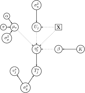
Graphical Representation of Equation (4)

Solid and dotted lines represent stochastic and deterministic dependencies, respectively.

Single-Marker Random-Effect Meta-Analysis

Results from the multilocus model are compared to those obtained from a more traditional single-locus random-effects meta-analysis in both simulation studies and with real data from the CRP-gene region. For the latter, a per-allele effect (95% CI) of individual SNPs on CRP concentration was derived from each individual study. The individual-study linear trend (additive effect) per category increase in genotype with mean data was calculated by simple linear regression, with genotypes coded as 0, 1, and 2 for homozygous common allele, heterozygous, and homozygous rare-allele, respectively, with the least-square linear-trend-coefficient formula, which only depends on the mean values and its standard deviations. A sensitivity analysis restricted to studies with more than 500 subjects, healthy at time of blood sampling, or to studies that reported all the required standard deviations was also conducted (Table S2). Subsequently, the study-specific linear trend and its standard error were pooled with random-effect models. Subsidiary analyses included pairwise comparisons within each polymorphism. The DerSimonian and Laird Q test, and the I² test,³² were used for evaluating the degree of heterogeneity between studies.

Results

Simulation Studies

We considered various scenarios differing in the number of studies and, for the multilocus approach, in the priors on the model space. Data were obtained as follows: We first simulated a pool of 4000 haplotypes at seven biallelic markers. Pairwise LD measures (r) between the seven SNPs are shown in Figure 3, with high LD only between the last three markers. SNP 6 is assumed to be the single causal site in the region and is retained in all subsequent analyses. Given the high LD between SNP 5, 6, and 7, we expect the results from the univariate analyses to be less conclusive than those from the multiple marker approach that adjusts for the between-marker correlations. The study size n_s was drawn from a normal distribution with mean 600 and variance 100, rounded to the nearest integer. Then, for subject $i\in \{1,\dots ,n^s\}$ and study s, a continuous phenotype y^s_i is simulated as

$$y_i^s={\beta }_0+{\beta }_6{g}_{i6}+{\mu }_s+{\varepsilon }_i$$ (6)

where g_i6 denotes the genotype of subject i at marker site 6 (0, 1, or 2 for homozygous wild-type, heterozygous, or homozygous mutant, respectively), (β₀, β₆) = (1, 2), μ_s ∼ N(0, 1), and ɛ ∼ N(0, 1). To reflect the fact that not all markers are typed in every study, we select at random m_s markers out of the possible seven for each study. Thus, in most cases the univariate analyses are based on fewer than the maximum total of S studies. For each simulated data set, we also estimated the unadjusted univariate additive effects and their standard errors at each SNP site; the additive effects are then combined in the univariate random-effect analyses.^33,34 Tables 1 and 2 present the results from the multiple-marker meta-analyses. The number of studies considered was 10, 20, or 40. In each case, the tables report the results obtained with Poisson priors on the model size in the reversible jump algorithm with different means (1 or 2 for priors a and b, respectively) or a uniform prior on the model space (prior c). Notice that the Poisson priors give more weight to the null model and may in general be a more reasonable choice in this setting. For example, prior a is Poisson(1) and assigns a probability of ∼0.26 of having more that one associated site (∼0.59 for b). The values shown are averages over 100 replicates. For each scenario, we report the marginal posterior probability of selecting each SNP and the mean and 95% credible intervals of the posterior distributions of each additive effect, conditional on the SNP being selected.^35,36 Note that posterior distributions can be reliably estimated only for markers with relatively high posterior probability of inclusion (e.g., >0.5), and results in the table should be interpreted with this in mind. The marginal probability of selecting the causal site is 1 independently of the prior used and even when considering as few as ten studies, with almost no variability across replicates. Notably, all other markers have posterior inclusion probabilities close to zero and would therefore not be selected if we were to use the traditional threshold of 0.5. All conditional mean additive effects are very close to the true values with a minor bias only for the effect at SNP 7, which is the SNP in highest LD with the causal site. The choice of prior distribution on model space does not have a large effect on the results, with possibly narrower credible intervals and slightly larger posterior probability of including SNP 7 under prior c compared to priors a and b. This is to be expected because the Poisson priors favor models with few terms, whereas the uniform prior gives equal weight to all models. The tables also report the results for the variance terms σ²_μ and σ²_y, which have posterior estimates close to the true values in both cases. Increasing the number of studies has little or no effect on both marginal posterior probabilities and posterior estimate bias but does lead to narrower credible intervals as expected.

Figure 3.

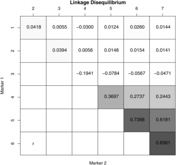
Pairwise LD Measures between Markers Used in the Simulation Study

Pairwise LD Measures are r values.

Table 1.

Bayesian Multilocus Meta-Analysis

		Parameter	β1	β2	β3	β4	β5	β6	β7	σ2y	σμ2
Number of Studies	Prior	True	0	0	0	0	0	2	0	1	1
		Post proba	0.01 (0.01)	0.01 (0.004)	0.01 (0.004)	0.005 (0.002)	0.01 (0.01)	1.00 (0.00)	0.03 (0.02)
	a	Meana	−0.01 (0.05)	−0.004 (0.04)	0.03 (0.03)	0.01 (0.03)	−0.01 (0.07)	2.00 (0.04)	0.16 (0.14)	1.19 (0.01)	1.25 (0.61)
		BCI length	0.19	0.20	0.15	0.14	0.35	0.19	0.76
		Post prob	0.02 (0.01)	0.01 (0.004)	0.01 (0.01)	0.01 (0.004)	0.02 (0.01)	1.00 (0.001)	0.07 (0.08)
10	b	Mean	−0.03 (0.04)	−0.01 (0.03)	0.03 (0.03)	0.02 (0.03)	−0.01 (0.08)	2.00 (0.05)	0.15 (0.16)	1.08 (0.02)	1.13 (0.34)
		BCI length	0.24	0.22	0.16	0.15	0.36	0.23	0.76
		Post prob	0.05 (0.02)	0.04 (0.02)	0.04 (0.02)	0.03 (0.01)	0.07 (0.03)	1.00 (0.001)	0.15 (0.05)
	c	Mean	−0.03 (0.04)	−0.01 (0.04)	0.02 (0.03)	0.01 (0.03)	−0.01 (0.07)	1.99 (0.04)	0.13 (0.12)	1.12 (0.01)	1.42 (0.46)
		BCI length	0.24	0.21	0.17	0.15	0.35	0.33	0.76
		Post prob	0.01 (0.01)	0.01 (0.002)	0.01 (0.003)	0.004 (0.002)	0.01 (0.003)	1.00 (0.00)	0.03 (0.08)
	a	Mean	−0.04 (0.03)	−0.02 (0.03)	0.03 (0.02)	0.01 (0.02)	−0.01 (0.05)	1.99 (0.04)	0.09 (0.10)	1.11 (0.01)	1.10 (0.26)
		BCI length	0.16	0.14	0.11	0.10	0.23	0.12	0.56
		Post prob	0.02 (0.02)	0.01 (0.01)	0.01 (0.01)	0.01 (0.003)	0.02 (0.01)	1.00 (0.001)	0.05 (0.04)
20	b	Mean	−0.04 (0.03)	−0.02 (0.03)	0.02 (0.03)	0.01 (0.02)	−0.02 (0.05)	1.99 (0.03)	0.13 (0.112)	1.06 (0.01)	1.08 (0.17)
		BCI length	0.16	0.15	0.12	0.10	0.24	0.17	0.57
		Post prob	0.06 (0.05)	0.03 (0.01)	0.03 (0.01)	0.02 (0.01)	0.06 (0.05)	1.00 (0.002)	0.13 (0.08)
	c	Mean	−0.05 (0.03)	−0.02 (0.02)	0.02 (0.02)	0.01 (0.02)	−0.01 (0.06)	1.99 (0.03)	0.10 (0.108)	1.09 (0.01)	0.99 (0.16)
		BCI length	0.18	0.15	0.12	0.11	0.26	0.23	0.59

^aResults are averages (std) over 100 replicated data sets. Mean posterior estimates and credible intervals are conditional on the SNP being included in a model.

Table 2.

Bayesian Multilocus Meta-Analysis

		Parameter	β1	β2	β3	β4	β5	β6	β7	σ2y	σμ2
Number of Studies	Prior	True	0	0	0	0	0	2	0	1	1
		Post prob	0.01 (0.15)	0.01 (0.003)	0.004 (0.002)	0.003 (0.001)	0.01 (0.004)	1 (0)	0.025 (0.28)
	a	Mean	−0.05 (0.02)	−0.03 (0.02)	0.02 (0.02)	0.01 (0.01)	−0.02 (0.04)	1.99 (0.02)	0.10 (0.08)	1.04 (0.01)	1.09 (0.14)
		BCI length	0.12	0.10	0.08	0.07	0.17	0.10	0.46
		Post prob	0.03 (0.03)	0.01 (0.01)	0.01 (0.00)	0.01 (0.002)	0.02 (0.01)	1 (0)	0.04 (0.03)
40	b	Mean	−0.05 (0.02)	−0.02 (0.02)	0.02 (0.02)	0.01 (0.02)	−0.03 (0.03)	1.99 (0.02)	0.12 (0.07)	1.03 (0.01)	0.97 (0.13)
		BCI length	0.12	0.11	0.08	0.07	0.19	0.12	0.46
		Post prob	0.07 (0.06)	0.03 (0.01)	0.02 (0.01)	0.01 (0.01)	0.04 (0.02)	1 (0)	0.11 (0.06)
	c	Mean	−0.05 (0.02)	−0.03 (0.02)	0.02 (0.02)	0.01 (0.01)	−0.01 (0.04)	1.99 (0.02)	0.10 (0.10)	1.03 (0.01)	1.01 (0.11)
		BCI length	0.12	0.11	0.10	0.077	0.19	0.18	0.48

Results are averages (std) over 100 replicated data sets. Mean posterior estimates and credible intervals are conditional on the SNP being included in a model.

The univariate analyses on the other hand fail to unambiguously identify the causal site at position 6 (Table 3). On the basis of results reported therein, although SNP 6 shows the highest association with the phenotype, SNP 7 could still be considered causal if no prior information is available to discriminate between the two. Even markers 4 and 5 would be selected on the basis of posterior credible intervals; paradoxically, increasing the number of studies only exacerbates the problem because credible intervals become narrower.

Table 3.

Single-Locus Random-Effects Meta-Analysis

	SNP ID	1	2	3	4	5	6	7
Number of Studies	True	0	0	0	0	0	2	0
	Mean (std)	−0.033 (0.028)	−0.023 (0.024)	0.069 (0.026)	0.312 (0.026)	1.158 (0.039)	1.990 (0.040)	1.945 (0.036)
10	Mean BCI length	0.385	0.379	0.367	0.365	0.414	0.434	0.482
	Mean (std)	−0.03 (0.018)	−0.019 (0.018)	0.072 (0.017)	0.314 (0.017)	1.169 (0.025)	1.999 (0.026)	1.942 (0.03)
20	Mean BCI length	0.258	0.253	0.245	0.244	0.269	0.286	0.327
	Mean (std)	−0.032 (0.014)	−0.021 (0.012)	0.067 (0.013)	0.311 (0.015)	1.165 (0.02)	1.998 (0.017)	1.94 (0.021)
40	Mean BCI length	0.183	0.179	0.175	0.175	0.194	0.203	0.23

Results are averages over 100 replicated data sets.

The previous simulation study assumed the same LD pattern across studies because study-specific genotype data are simulated from a common haplotype pool. To mimic a more realistic scenario, we further considered study-specific LD patterns by simulating genotype counts from study-specific haplotype pools characterized by slightly different LD structures. The multilocus analysis then uses the average LD table shown in Figure D1 (in which we also report the standard deviations of the pairwise r² values across studies in brackets). Results are reported in Table 4 for replicates with 20 studies. The method appears to be fairly robust to minor deviations in LD patterns across studies (similar to those observed for the real data in the next section); large differences in LD structures across studies would necessarily invalidate the meta-analytical approach because there would be little information to borrow for variable selection.

Table 4.

Bayesian Multilocus Meta-Analysis when the LD Structure Is Allowed to Vary across Studies

Number of studies		Parameter	β1	β2	β3	β4	β5	β6	β7	σ2y	σμ2
	Prior	True	0	0	0	0	0	2	0	1	1
		Post prob	0.01 (0.01)	0.01 (0.01)	0.03 (0.02)	0.03 (0.06)	0.01 (0.01)	1.00 (0.00)	0.03 (0.03)
	a	Mean	−0.02 (0.04)	−0.02 (0.03)	0.07 (0.01)	0.04 (0.04)	−0.01 (0.06)	1.97 (0.01)	0.13 (0.11)	1.06 (0.02)	1.07 (0.23)
		BCI length	0.16	0.15	0.10	0.10	0.23	0.14	0.58
		Post prob	0.01 (0.01)	0.01 (0.01)	0.02 (0.01)	0.01 (0.01)	0.02 (0.01)	1.00 (0.00)	0.08 (0.05)
20	b	Mean	−0.01 (0.04)	0.01 (0.04)	0.06 (0.02)	−0.02 (0.04)	−0.01 (0.07)	1.98 (0.04)	0.14 (0.28)	1.08 (0.02)	1.03 (0.13)
		BCI length	0.2	0.12	0.15	0.15	0.32	0.29	0.67
		Post prob	0.03 (0.01)	0.03 (0.01)	0.11 (0.13)	0.10 (0.08)	0.04 (0.05)	1.00 (0.00)	0.12 (0.04)
	c	Mean	−0.02 (0.03)	−0.02 (0.02)	0.05 (0.03)	0.04 (0.04)	0.01 (0.04)	1.99 (0.03)	0.15 (0.05)	1.04 (0.01)	1.07 (0.12)
		BCI length	0.17	0.15	0.12	0.10	0.22	0.24	0.58

Results are averages (std) over 100 replicated data sets. Mean posterior estimates and credible intervals are conditional on the SNP being included in a model. See Figure D1.

Finally, we considered reducing the effect at the causal site to 1.5 or placing it at marker position 2, which is in linkage equilibrium with the other sites: In both cases, the causal site is selected with high posterior probability (>0.8, results not shown).

The WinBUGS code used to fit the model is given in Appendix C.

A Meta-Analysis of CRP Studies

The traditional single-locus meta-analyses require that the available data be partitioned into groups of studies in which the same SNP was typed directly. In these analyses, seven SNPs were associated with a codominant effect on CRP concentration (Figure 4) with the per-allele effect in the range of 0.19–0.58 mg/L (absolute p values: rs1800947 = 4.35 × 10⁻⁹; rs1205 = 7.76 × 10⁻²⁶; rs1417938 = 1.77 × 10⁻²; rs1130864 = 2.73 × 10⁻¹¹; rs3091244 = 4.50 × 10⁻¹⁵; rs3093077 = 5.03 × 10⁻¹¹; and rs3093059 = 2.27 × 10⁻⁸), corresponding to ∼0.3–0.8 SD of the population distribution of CRP 37. The main effect estimates were robust to analyses limited to studies of >500 subjects (Table S2), providing strong evidence for an association at this locus. However, because pooled analyses of this type are limited to individual SNPs, it is unclear which of these SNPs have independent effects and which are associated because of correlation with other observed or unobserved SNPs, including the true causal variant(s). This can be overcome by incorporating available information on pairwise LD in the region (Table S3) within a Bayesian multilocus model as described above. Bayesian model selection can then facilitate identification of variants showing the strongest independent association with CRP concentration (Figure 5 and Table 5). The approach yields posterior model probabilities conditional on the observed data from which marginal probabilities of association for each SNP can be readily obtained. Of the markers considered, SNPs rs1130864, rs1205, and rs3093077, all in the 3 UTR, retain the strongest independent association with CRP concentration. An additional synonymous SNP in exon 2 (rs1800947) appears to be important, although its posterior probability of association is sensitive to the prior on the model space, and becomes unimportant if a more restrictive prior on the number of associated markers in the region is used (results not shown). These four SNPs yield the model with the highest posterior probability (Figures 4 and 5 and Table 5). Again, the models were not materially altered when analyses were limited to studies of >500 subjects (results not shown).

Figure 4.

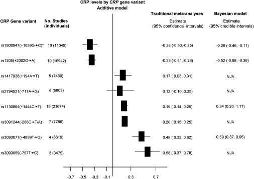
Summary Effect from Traditional Meta-Analysis and Bayesian Multiple-SNP Hierarchical Linear Model of the Eight SNPs in the CRP Gene

Values shown are additive genetic effects on (log) CRP levels with 95% confidence intervals or credible intervals for traditional and Bayesian analyses, respectively. For the Bayesian analysis, results are shown only for those markers that appear to be strongly associated after variable selection (see Figure 5). N/A refers to SNPs excluded from the model. The asterisk indicates the dominant model. Negative values indicate the variant allele is associated with a lower CRP concentration.

Figure 5.

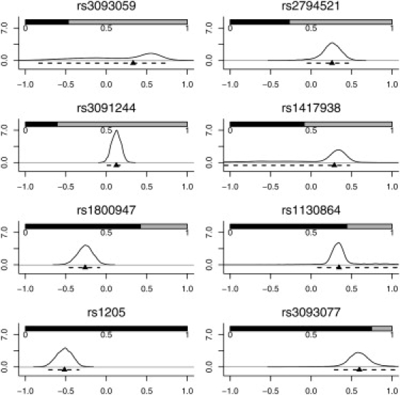
Results from the Multiple-SNP Meta-Analysis using the Bayesian Hierarchical Linear Model

The shaded bars show the posterior probability that each SNP is included in a model, calculated from the posterior sample of models. The x axis indicates the additive effects of each SNP on log CRP plasma levels, conditional on that SNP being included in the model, and the y axis indicates the corresponding posterior density. The curves can thus be interpreted as smoothed histograms representing the probability that the SNP effects take the values on the x axis. Also shown are the densities, medians (▴), and 95% credible intervals (- - -) for the additive effects of each SNP on log CRP levels.

Table 5.

Application to the Meta-Analysis of CRP Studies

Prob	SNP included
	rs3093059	rs2794521	rs3091244	rs1417938	rs1800947	rs1130864	rs1205	rs3093077
0.22					•	•	•	•
0.12						•	•	•
0.10				•	•		•	•
0.07					•		•	•
0.06		•			•	•	•	•

Models with more than 2% posterior probability are shown. Results assume a Poisson(2) prior on model size in the reversible jump algorithm.

Notably, SNPs rs1130864, rs1205, and rs3093077 formed the trio of tag SNPs. Because each tag SNP marks a different haplotype, the Bayesian model implies the presence of at least three functional SNPs regulating CRP level (Figure 6). Using HapMap, we found that there were 11 SNPs in strong LD with rs1205, (five with pairwise r² = 1) within an associated interval of ∼100 kb. There were 11 SNPs in strong LD with rs3093077 (nine with pairwise r² = 1), within a larger associated interval of ∼300 kb. A total of 22 SNPs lay in an associated interval of 100 kb encompassing rs1130864 (nine with pairwise r² = 1) (Figure 7). Because tightly linked SNPs were identified in the associated intervals, a careful assessment of potential functionality for each of these SNPs is now required.

Figure 6.

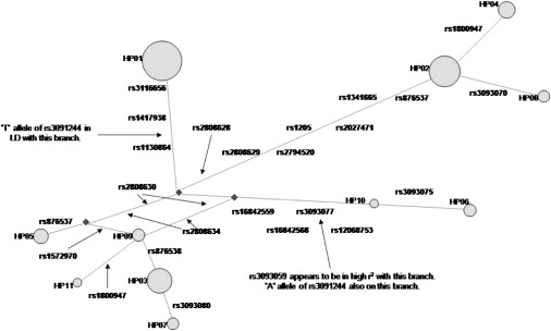
A Reduced Median Network Constructed with HapMap CEPH Data for a 20 kb Region Containing the CRP Gene

Yellow circles indicate haplotypes. The size of each circle is proportional to the frequency of that haplotype in the HapMap CEPH population. Non-HapMap SNPs (indicated in italics) were placed on the network with information from other CEPH populations.

Figure 7.

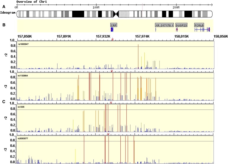
Genomic Context for CRP Gene

(A) Ideogram depicting the chromosome and region in which the CRP gene lies (red line).

(B) Gene diagram with introns and exons depicted as horizontal and vertical blue lines, respectively.

(C) Pairwise r² LD values between independently associating SNPs from Bayesian analysis (identified in top left of window, position indicated by red arrow) and all other HapMap SNPs in the region (release 20, build 35, red = r² > 0.8, yellow = 0.5 < r² < 0.8, gray = 0.3 < r² < 0.5, blue = 0.2 < r² < 0.3, and dark gray = missing data).

As mentioned in the previous section, in order to accommodate outliers and heavy tails, we assumed the distribution of the between-studies random effects μ_s to be a mixture of normals. In particular, inspection of the residuals from a model fitted without the between-studies random effect appears to suggest the use of a two-component mixture, see Figure 8. The graph plots a sample of the quantities

$$r_j^s=T_j^s-{\mathbf{W}}_{\mathit{j},}.{{}^{\left(t\right)}\beta }^{\left(t\right)}-U_j^{\left(t\right)}$$ (7)

for current values of the spatial random effects U and model at iteration t.²⁸ The posterior distribution of α₁ and α₂ had means of −0.014 and 3.356, respectively (Figure 8), whereas π had posterior median estimate of 0.879. By monitoring the mixture component assignments of each study, we found that outlying studies were mostly assigned to the second component as expected (results not shown).

Figure 8.

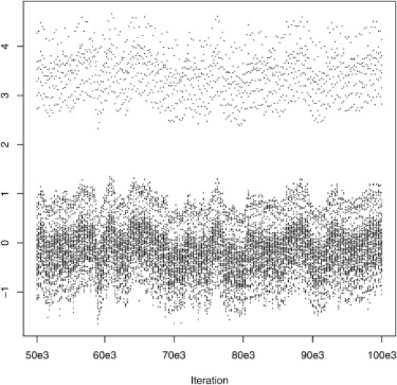
Posterior Sample of Residuals from the Hierarchical Model of Material and Methods Fitted without the Between-Study Random-Effect Term μ_s

Discussion

With only small genetic effects expected to contribute to most complex diseases, the meta-analysis of studies that consider variants in the same genetic region is a promising strategy to increase our chances of finding any associations. Recognizing the importance of this approach, several coordinated efforts have been initiated to ensure that results from the individual studies follow agreed guidelines and can be combined more easily.⁷

Most of the meta-analyses conducted so far have considered each marker in isolation, ignoring the possible correlation between markers due to linkage disequilibrium that reduces efficiency and that compromises the identification of any causal site. In this paper, we have presented a multimarker approach that yields estimates of effect at each site adjusted for the effects of other variants, as in multiple regression. In both the simulation study and the application to the CRP data, we assumed an additive genetic model. Other choices are possible and would only involve changes in the entries of the matrices W and X′X.

The methods borrow from the spatial data literature and incorporate the prior knowledge of marker pairwise LD in a fully Bayesian framework. For example, similar hierarchical models with spatial random effects are used extensively in the analysis of spatial epidemiological data. A convenient feature of the joint specification (Equation [3]) is that it allows incorporation of the required correlation structure as prior information in an explicit way.^13,37 In addition, a reversible jump algorithm on the space of possible model structures enables the selection of the most promising associations. The proposed approach assumes data on a continuous phenotype. However, it could be extended to the case of discrete outcomes, say case-control status, by introducing a further set of continuous latent variables related to the discrete outcome as in probit regression. Extensions to include metaregression are straightforward and only involve introduction of a further hierarchy for the vector of coefficients β in Equation (4) with means that would then depend on study-specific covariates. Work on these extensions is currently in progress.

When applied to the meta-analysis of studies in the CRP-gene region, results provide evidence for three CRP modifying alleles distributed over three of four common haplotypes in Europeans. These alleles could account for the strong association with CRP of each of the three SNPs that are chosen for their ability to tag others and that mark the different haplotypes. The associated interval for each independently associating SNP extended at least 100 kb from either side of the open reading frame with a very sharp boundary of LD for at least two of these. Within each interval were a number of additional candidate causal SNPs in complete LD with the index SNP from the Bayesian analysis, any of which could, in theory, regulate CRP. Although the A and T alleles of the triallelic SNP rs3091244 appeared to exhibit functionality in previous reporter-gene studies in vitro,²¹ this SNP was not retained within the Bayesian model. Experimental studies of this type may be biased toward the study of potential regulatory SNPs in the immediate vicinity against those located remotely from the gene of interest because of size constraints on reporter-gene constructs. This might explain why results of such reporter studies are, at times, discordant with the findings of association analyses in populations³⁸ or alternative experimental approaches to assessing functionality.³⁹ Irrespective of the true causal sites, the three tag SNPs adequately capture functional variation at this locus for large-scale gene-disease association studies. Although the naive expectation would be of narrower limits of error around the point estimates of SNP effects with a Bayesian approach that includes all studies simultaneously, this was not observed. This is because unlike the traditional meta-analyses, the Bayesian analyses were corrected for the effect of other SNPs; that is, uncertainty about which SNPs are directly associated with the trait was properly incorporated in the analyses. However, the simultaneous use of all data strengthens evidence for an association at the gene level; the null model does not appear at all in the posterior sample of models, reflecting virtual certainty of an effect on CRP at this gene.

Our approach facilitates the integration of data from studies that have genotyped different SNPs across the same gene or region utilizing prior information on LD. It has a number of favorable attributes and potential applications. By increasing the available data set of information on any SNP, the efficiency of evidence synthesis is enhanced and the reliability of any identified associations is increased. Further, the variable selection procedure allows inference on the relative magnitude of any marker-phenotype association and identifies those SNPs that show the strongest association with the phenotype, either because they are the functional site(s) or because they exhibit the strongest allelic association with (unobserved) functional sites. IPD (where available) can also be incorporated readily into the analysis because the regression parameters measuring the effect of variants retain the same interpretation when considering aggregate data (i.e., phenotype means by genotype groups as with CRP studies) or IPD (see Material and Methods). Moreover, where a robust evidence based on genetic association with a quantitative trait already exists (as it does for many blood measures, e.g., HDL cholesterol, triglycerides, and others), the methods described could be used to add and integrate partially overlapping SNP data from new genome-wide analyses, thereby harnessing existing data for both replication, and to gain insight into likely causal sites in a gene or region. The methods we describe, which use the freely available software WinBUGS, are likely to be of substantial value both to the emerging networks of investigators engaged in synthesis of evidence on genetic associations of complex quantitative traits and disorders⁷ and to those applying and extending findings from genome-wide association studies.

Appendix A

Systematic Review

Two electronic databases (PubMed Medline and EMBASE) were searched with the text words, which were also MeSH terms, polymorphism(s), mutation(s), gene(s), genetic, variant(s), and SNP(s) in combination with C-reactive protein and CRP. The literature search was limited to human and to the English language. Any additional studies in the references of all identified publications were also searched. For inclusion, studies had to have an analytical design (case control, prospective, or cross sectional) and examine the association between any polymorphisms in the CRP gene and low-chronic CRP concentrations in individuals of European descent. Studies measuring CRP only during acute phase of an inflammatory response (e.g., acute ischemia or infection stimuli) were excluded. In areas where more than one polymorphism had been studied, information about the LD between them was extracted where available. If relevant information was not reported (mean CRP levels, standard deviations, genotype numbers, or linkage disequilibrium data), or it was not reported stratified by ethnicity, the authors were contacted in several occasions to obtain the information. A total of four potential studies (n = 2614) in European subjects were excluded because of unavailability of data in the appropriate form (Flex 2004, n = 471; Obisesan 2004, n = 63; Zee 2004, n = 260; Carlson 2005, n = 1820) (see Table S1).

New Data Sets

NPHS II is a prospective study of 3012 healthy white European middle-aged men, of which a total of 2479 with CRP genetic data and CRP concentrations were included in this report. Recruitment in the study commenced in 1989⁴⁰ in nine general practices. None of the participants had a clinical history of unstable angina, myocardial infarction (including silent infarction), coronary surgery, other cardiovascular diseases, aspirin or anticoagulant use, or malignant disease (except skin cancer other than melanoma) at the time of recruitment. The Ely Study is a prospective population-based cohort study of the etiology and pathogenesis of type 2 diabetes and related metabolic disorders in 1122 individuals recruited in 1990 in Ely, Cambridgeshire.⁴¹ Complete data on biochemical and anthropometric variables were available in 839 participants, and a total of 548 individuals with data on the CRP genotypes and CRP levels were included in this analysis. The EPIC-Norfolk study is a population-based cohort study, recruiting participants from general practices in Norfolk.⁴² For the present report, only control participants from a nested case-control study in coronary heart disease were included, providing a total of 2196 participants with both data on CRP genetic variants and CRP concentrations.

New Genotyping

Polymorphisms in the human CRP gene (HGNC: 2637; 1q21-q23) were identified by reference to public-domain databases of human sequence variation. We used this information to generate a consensus map of polymorphic sites. By using validated genotype data (minor allele frequency >5%) from subjects of European descent from the SeattleSNPs database and the human HapMap database (see Web Resources), we examined the pattern of linkage disequilibrium across the CRP gene. We then used the haplotype LD r² method to select a set of tagging (t)SNPs capable of capturing maximum haplotype diversity among subjects of European descent by using the program TagIT (see Web Resources).

LD

Public domain databases (see Web Resources) and individual publications were examined for information on the LD structure in the CRP gene. Both D′ and r² values were recorded, but r² values were utilized in Bayesian modeling. If more than one r² value for a given pairwise was reported, a weighted mean r² was obtained.

Appendix B

Recovering the Joint Distribution of Multiallelic Sites from Allele Frequencies and Marginal Diallelic r² Values

We consider two loci, the first locus having G₁ = three alleles and the second locus having G₂ = two alleles. The joint probability of the haplotypes at these two loci can be represented in a 3 × 2 table of the form:

Table B1.

Full 3 × 2 Table of Haplotype Probabilities

Allele at Locus 1	Allele at Locus 2
	1	2
1	p11	P1 − p11	P1
2	p21	P2 − p21	P2
3	Q1 − p11 − p21	(1 − Q1) − (P1 − p11) − (P2 − p21)	(1 − P1 − P2)
	Q1	(1 − Q1)	1

where p_ij denotes the joint probability of allele i at locus 1 and allele j at locus 2, P_i denotes the probability of allele i at locus 1, and Q₁ denotes the probability of allele 1 at locus 2.

The internal cells of this table are not observed. Our problem is to derive this table of probabilities on the basis of information from the margins of this table (P₁, P₂ and Q₁) and pair-wise correlation within two marginal tables of the form:

Table B2.

First Marginal 2 × 2 Haplotype Table

	Allele at Locus 2
Allele at Locus 1	1	2
1	p′11	P′1 − p′11	P′1
3	Q′1 − p′11	(1 − Q′1) − (P′1 − p′11)	(1 − P′1)
	Q′1	(1 − Q′1)	1

and

Table B3.

Second Marginal 2 × 2 Haplotype Table

	Allele at Locus 2
Allele at Locus 1	1	2
2	p″21	(P″2 − p″21)	P″2
3	Q″1 − p″21	(1 − Q″1) − (P″2 − p″21)	(1 − P″2)
	Q″1	(1 − Q″1)	1

In the first of these tables, p′₁₁ denotes the joint probability of allele 1 at locus 1 and allele 1 at locus 2, but now this probability is conditional upon the allele at locus 1 having either a 1 or 3 allele. Similarly, p₂₁ denotes the probability of allele 2 at locus 1 and allele 1 at locus 2 conditional upon the allele at locus 1 being either a 2 or a 3.

We do not observe the two tables above but only the appropriate deviations from linkage disequilibrium, δ′₁₃ and δ″₂₃, defined by

$${\delta }_{13}={P^{\prime }}_1\ast {Q^{\prime }}_1-{p^{\prime }}_{11}$$

and

$${\delta \prime }_{23}={P″}_2\ast {Q″}_1-{p″}_{21}.$$

We know that the probability of each pair-wise haplotype in Table 2 is equal to the corresponding probability of that pairwise haplotype in Table 1, divided by the probability that the allele at the first locus is either equal to 1 or 3, (1 − P₂). This means that:

$${p\prime }_{11}=\frac{p_{11}}{(1-P_2)}$$

and

$$({Q\prime }_1-{p\prime }_{11})=\frac{(Q_1-p_{11}-p_{21})}{(1-P_2)}.$$

Therefore,

$$\begin{array}{l}{Q\prime }_1=\frac{(Q_1-p_{11}-p_{21})}{(1-P_2)}+\frac{p_{11}}{(1-P_2)}\hfill \\ =\frac{(Q_1-p_{21})}{(1-P_2)},\hfill \end{array}$$

and

$$p_{11}=p_{11}(1-P_2).$$

Following a similar argument, we also find that

$${Q″}_1=\frac{(Q_1-p_{11})}{(1-P_1)}$$

and

$$p_{21}=p_{21}(1-P_1).$$

By writing p′₁₁ and p″₂₁ in terms of δ′₁₃ and δ″₂₃, we find that:

$$\begin{array}{l}{p}_{11}={p\prime }_{11}(1-P_2)\hfill \\ =({P\prime }_1\ast {Q\prime }_1-{\delta \prime }_{11})(1-P_2)\hfill \\ =\left(\frac{P_1}{(1-P_2)}\frac{(Q_1-p_{21})}{(1-P_2)}-{\delta \prime }_{11}\right)(1-P_2)\hfill \\ =\frac{1}{(1-P_2)}\left(P_1{Q}_1-P_1{p}_{21}-{\delta \prime }_{11}{(1-P_2)}^2\right)\hfill \end{array}$$

and

$$\begin{array}{l}{p}_{21}={p\prime }_{21}(1-P_1)\hfill \\ =({P″}_2\ast {Q″}_1-{\delta \prime }_{21})(1-P_1)\hfill \\ =\left(\frac{P_2}{(1-P_1)}\frac{(Q_1-p_{11})}{(1-P_1)}-{\delta ″}_{21}\right)(1-P_1)\hfill \\ =\frac{1}{(1-P_1)}\left(P_2{Q}_1-P_2{p}_{11}-{\delta ″}_{21}{(1-P_1)}^2\right).\hfill \end{array}$$

This means that we have two equations in two unknowns, p₁₁ and p₂₁, so that by substituting the second equation for p₂₁ into the first equation for p₁₁, we can then solve this equation in terms of p₁₁. Substituting the expression for p₁₂ into that for p₁₁ gives:

$$\begin{array}{l}{p}_{11}=\frac{1}{(1-P_2)}\left(P_1{Q}_1-P_1{p}_{21}-{\delta \prime }_{11}{(1-P_2)}^2\right)\hfill \\ =\frac{1}{(1-P_2)}\left(P_1{Q}_1-\frac{P_1}{(1-P_1)}\left(P_2{Q}_1-P_2{p}_{11}-{\delta ″}_{21}{(1-P_1)}^2\right)-{\delta \prime }_{11}{(1-P_2)}^2\right),\hfill \end{array}$$

and rearranging in terms of p₁₁ results in the equation:

$$p_{11}=P_1{Q}_1+\frac{(1-P_1)}{(1-P_1-P_2)}\left(P_1(1-P_1){\delta ″}_{21}-{(1-P_2)}^2{\delta \prime }_{11}\right).$$

We may then write p₂₁ in the form

$$p_{21}=P_2{Q}_1+\frac{(1-P_2)}{(1-P_1-P_2)}\left(P_2(1-P_2){\delta \prime }_{11}-{(1-P_1)}^2{\delta ″}_{21}\right).$$

We are now able to calculate the probability of every cell of Table B1 in terms of p₁₁, p₁₂, P₁, P₂, and Q₁.

Note that δ′₁₁ and δ″₂₁ can be obtained from the relevant r² values with the formulae:

$${\delta \prime }_{11}=(+/-)\sqrt{{\left({r\prime }_{11}\right)}^2{P\prime }_1(1-{P\prime }_1){Q\prime }_1(1-{Q\prime }_1)}$$

and

$${\delta ″}_{21}=(+/-)\sqrt{{\left({r″}_{21}\right)}^2{P″}_2(1-{P″}_2){Q″}_1(1-{Q″}_1)}.$$

Care must be taken when choosing which sign to assign these δ values because they must be consistent with the margins of the Tables B2 and B3.

Appendix C

WinBUGS Code for the Model Described in Material and Methods

model {

# likelihood

for(j in 1:Q) {# where $Q={\sum }_s(m_s+1)$

T[j] ∼dnorm(theta[j],tauy[j])

tauy[j] ← tau.y/XsXs[j] # XsXs[j] in Equation (4)

theta[j] ← psi[j]+sumXis[j]^∗mu[study[j]]+U[marker[j]] # linear predictor in Equation (4)

}

# pooled variances

for(i in 1:L) {# where $L={\sum }_s{m}_s$

scale[i] ← tau.y/2

shape[i] ← pooled[i,2]/2

pooled[i,1] ∼dgamma(shape[i],scale[i]) # uses the gamma parameterization

}

#reversible jump part as detailed in Lunn et al.²⁵

psi[1:Q] ← jump.lin.pred(W[1:Q,1:m],K,tau.beta)

id ← jump.model.id(psi[1:Q])

pred[1:(m+1)] ← jump.lin.pred.pred(psi[1:Q],X.pred[1:(m+1),1:m])

for(i in 1:m){

X.pred[i,i] ← 1

for(j in 1:(i−1)) {X.pred[i,j] ← 0}

for(j in (i+1):m) {X.pred[i,j] ← 0}

X.pred[(m+1),i] ← 0

effect[i] ← pred[i] -pred[m+1]

}

# mixture distribution for study effects

for(s in 1:nstudies) {

mu[s] ∼dnorm(mumu[s],tau.mu)

mumu[s] ← alpha[comp[s]]

comp[s] ∼dcat(phi[])

}

phi[2] ← 1-phi[1]

alpha[2] ← (-phi[1]^∗alpha[1])/(1-phi[1])

# prior distributions

U[1:m] ∼car.proper(thetaU[],M[],adj[],num[],m[],prec,1)

# thetaU vector of zeros of length m (number of unique markers)

# M is weighted average of the X^s′X^s matrices

# details on vectors adj, num and m are given in the manual for GeoBUGS

prec ∼dgamma(0.5,0.0005)

tau.y ∼dgamma(0.001,0.001)

tau.mu ∼dgamma(0.001,0.001)

tau.beta ∼dgamma(0.0001,0.0001)

phi[1] ∼dbeta(1,1)

alpha[1] ∼dnorm(0.0,1.0E-6)

K ∼dpois(1) # scenario (a)

}

The MCMC chain was run for 1,000,000 iterations with a burn-in of 500,000 and thinning of 100 iterations, which took ∼30 min of CPU time on an Itel Xeon 2.80 GHz with 2 GB of RAM. Convergence was checked by visual inspection of posterior traces and by running chains with different initial values.³⁶

Appendix D

Figure D1.

Mean Pairwise LD Measures between Markers Used in the Simulation Study when Allowing LD Patterns to Vary across Studies

Supplemental Data

Three tables are available at http://www.ajhg.org/.

Web Resources

The URLs for data presented herein are as follows:

• CRP:C-reactive protein, pentraxin-related, http://pga.gs.washington.edu/data/crp/

• HapMap homepage, http://www.hapmap.org/

• Online Mendelian Inheritance in Man (OMIM), http://www.ncbi.nlm.nih.gov/Omim

• TagIT, http://popgen.biol.ucl.ac.uk/software.html

• WinBUGS software, http://www.mrc-bsu.cam.ac.uk/bugs/winbugs/contents.shtml

References

- 1.Cardon L., Bell J. Association study designs for complex diseases. Nat. Rev. Genet. 2001;2:91–99. doi: 10.1038/35052543. [DOI] [PubMed] [Google Scholar]
- 2.Colhoun H., McKeigue P., Davey Smith G. Problems of reporting genetic associations with complex outcomes. Lancet. 2003;361:865–872. doi: 10.1016/s0140-6736(03)12715-8. [DOI] [PubMed] [Google Scholar]
- 3.Clayton D., McKeigue P. Epidemiological methods for studying genes and environmental factors in complex diseases. Lancet. 2001;358:1356–1360. doi: 10.1016/S0140-6736(01)06418-2. [DOI] [PubMed] [Google Scholar]
- 4.Zeggini E., Rayner W., Morris A.P., Hattersley A.T., Walker M., Hitman G.A., Deloukas P., Cardon L.R., McCarthy M.I. An evaluation of hapmap sample size and tagging snp performance in large-scale empirical and simulated data sets. Nat. Genet. 2005;37:1320–1322. doi: 10.1038/ng1670. [DOI] [PubMed] [Google Scholar]
- 5.Cambon-Thomsen A. Assessing the impact of biobanks. Nat. Genet. 2003;34:25–26. doi: 10.1038/ng0503-25b. [DOI] [PubMed] [Google Scholar]
- 6.Little J., Bradley L., Bray M., Clyne M., Dorman J., Ellsworth D., Hanson J., Khoury M., Lau J., O'Brien T. Reporting, appraising, and integrating data on genotype prevalence and gene-disease associations. Am. J. Epidemiol. 2002;156:300–310. doi: 10.1093/oxfordjournals.aje.a000179. [DOI] [PubMed] [Google Scholar]
- 7.Ioannidis J.P., Gwinn M., Little J., Higgins J.P., Bernstein J.L., Boffetta P., Bondy M., Bray M.S., Brenchley P.E., Buffler P.A. A road map for efficient and reliable human genome epidemiology. Nat. Genet. 2006;38:3–5. doi: 10.1038/ng0106-3. [DOI] [PubMed] [Google Scholar]
- 8.Seminara D., Khoury M., O'Brien T., Manolio T., Gwinn M., Little J., Higgins J., Bernstein J., Boffetta P., Bondy M. The emergence of networks in human genome epidemiology: Challenges and opportunities. Epidemiology. 2007;18:1–8. doi: 10.1097/01.ede.0000249540.17855.b7. [DOI] [PubMed] [Google Scholar]
- 9.Scott L., Mohlke K., Bonnycastle L., Willer C., Li Y., Duren W., Erdos M., Stringham H., Chines P., Jackson A. A genome-wide association study of type 2 diabetes in finns detects multiple susceptibility variants. Science. 2007;316:1341–1345. doi: 10.1126/science.1142382. [DOI] [PMC free article] [PubMed] [Google Scholar]
- 10.Dina C., Meyre D., Gallina S., Durand E., Krner A., Jacobson P., Carlsson L., Kiess W., Vatin V., Lecoeur C. Variation in fto contributes to childhood obesity and severe adult obesity. Nat. Genet. 2007;39:724–726. doi: 10.1038/ng2048. [DOI] [PubMed] [Google Scholar]
- 11.The Wellcome Trust Case – Control Consortium Genome – wide association study of 14,000 cases of seven common diseases and 3,000 shared controls. Nature. 2007;447:661–678. doi: 10.1038/nature05911. [DOI] [PMC free article] [PubMed] [Google Scholar]
- 12.Besag J., Kooperberg C.L. On conditional and intrinsic autoregressions. Biometrika. 1995;82:733–746. [Google Scholar]
- 13.Lawson A.B. John Wiley; Chichester, UK: 2001. Statistical Methods in Spatial Epidemiology. [Google Scholar]
- 14.Hirschfield G., Pepys M. C-reactive protein and cardiovascular disease: new insights from an old molecule. QJM. 2003;96:793–807. doi: 10.1093/qjmed/hcg134. [DOI] [PubMed] [Google Scholar]
- 15.Danesh J., Wheeler J., Hirschfield G., Eda S., Eiriksdottir G., Rumley A., Lowe G., Pepys M., Gudnason V. C-reactive protein and other circulating markers of inflammation in the prediction of coronary heart disease. N. Engl. J. Med. 2004;350:1387–1397. doi: 10.1056/NEJMoa032804. [DOI] [PubMed] [Google Scholar]
- 16.Hingorani A., Humphries S. Nature's randomised trials. Lancet. 2005;366:1906–1908. doi: 10.1016/S0140-6736(05)67767-7. [DOI] [PubMed] [Google Scholar]
- 17.Hingorani A., Shah T., Casas J. Linking observational and genetic approaches to determine the role of c-reactive protein in heart disease risk. Eur. Heart J. 2006;27:1261–1263. doi: 10.1093/eurheartj/ehi852. [DOI] [PubMed] [Google Scholar]
- 18.Davey Smith G., Ebrahim S. Mendelian randomization: Can genetic epidemiology contribute to understanding environmental determinants of disease? Int. J. Epidemiol. 2003;32:1–22. doi: 10.1093/ije/dyg070. [DOI] [PubMed] [Google Scholar]
- 19.Davey Smith G., Ebrahim S. Mendelian randomization: Prospects, potentials and limitations. Int. J. Epidemiol. 2004;33:30–42. doi: 10.1093/ije/dyh132. [DOI] [PubMed] [Google Scholar]
- 20.MacGregor A., Gallimore J., Spector T., Pepys M. Genetic effects on baseline values of c-reactive protein and serum amyloid a protein: A comparison of monozygotic and dizygotic twins. Clin. Chem. 2004;50:130–134. doi: 10.1373/clinchem.2003.028258. [DOI] [PubMed] [Google Scholar]
- 21.Carlson C., Aldred S., Lee P., Tracy R., Schwartz S., Rieder M., Liu K., Williams O., Iribarren C., Lewis E. Polymorphisms within the c-reactive protein (crp) promoter region are associated with plasma crp levels. Am. J. Hum. Genet. 2005;77:64–77. doi: 10.1086/431366. [DOI] [PMC free article] [PubMed] [Google Scholar]
- 22.Kardys I., de Maat M., Uitterlinden A., Hofman A., Witteman J. C-reactive protein gene haplotypes and risk of coronary heart disease: The rotterdam study. Eur. Heart J. 2006;27:1331–1337. doi: 10.1093/eurheartj/ehl018. [DOI] [PubMed] [Google Scholar]
- 23.Marchini J., Howie B., Myers S., McVean G., Donnelly P. A new multipoint method for genome-wide association studies by imputation of genotypes. Nat. Genet. 2007;39:906–913. doi: 10.1038/ng2088. [DOI] [PubMed] [Google Scholar]
- 24.Green P. Reversible jump markov chain monte carlo computation and bayesian model determination. Biometrika. 1995;82:711–732. [Google Scholar]
- 25.Lunn D., Whittaker J., Best N. A bayesian toolkit for genetic association studies. Genet. Epidemiol. 2006;30:231–247. doi: 10.1002/gepi.20140. [DOI] [PubMed] [Google Scholar]
- 26.Thomas D. Oxford University Press; New York: 2004. Statistical Methods in Genetic Epidemiology. [Google Scholar]
- 27.Besag J., York J., Mollie A. Bayesian image restoration, with two applications in spatial statistics (with discussion) Ann. Inst. Stat. Math. 1991;43:1–59. [Google Scholar]
- 28.Dominici F., Parmigiani G., Wolpert R.L., Hasselblad V. Meta-analysis of migraine headache treatments: Combining information from heterogeneous designs. J. Am. Stat. Assoc. 1999;94:16–28. [Google Scholar]
- 29.Kelsall, J., and Wakefield, J.C. (1999). Comment on Bayesian models for spatially correlated disease and exposure data. In Bayesian Statistics 6 Proceedings of the Sixth Valencia International Meeting (Oxford: Clarendon Press).
- 30.Denison D.G.T., Holmes C.C., Mallick B.K., Smith A.F.M. John Wiley; Chichester, UK: 2002. Bayesian Methods for Nonlinear Classification and Regression. [Google Scholar]
- 31.Verzilli C.J., Whittaker J.C., Stallard N. A hierarchical bayesian model for predicting the functional consequences of amino acid polymorphisms. J. R. Stat. Soc. Ser. C Appl. Stat. 2005;54:191–207. [Google Scholar]
- 32.Higgins J., Thompson S., Deeks J., Altman D. Measuring inconsistency in meta-analyses. BMJ. 2003;327:557–560. doi: 10.1136/bmj.327.7414.557. [DOI] [PMC free article] [PubMed] [Google Scholar]
- 33.DuMouchel W.H. Statistical Methodology in the Pharmaceutical Sciences. Marcel Dekker; New York: 1990. Bayesian meta-analysis. [Google Scholar]
- 34.Normand S.L.T. Meta-analysis: Formulating, evaluating, combining and reporting. Stat. Med. 1999;18:321–359. doi: 10.1002/(sici)1097-0258(19990215)18:3<321::aid-sim28>3.0.co;2-p. [DOI] [PubMed] [Google Scholar]
- 35.O'Hagan A., Forster J. Kendall's Advance Theory of Statistics. Vol 2B. Arnold; London: 2004. Bayesian Inference. [Google Scholar]
- 36.Carlin B.P., Louis T.A. Chapman & Hall; Boca Raton: 2002. Bayes and Empirical Bayes Methods for Data Analysis. [Google Scholar]
- 37.Parent O., Riou S. Bayesian analysis of knowledge spillovers in european regions. J. Reg. Sci. 2005;45:747–775. [Google Scholar]
- 38.Ioannidis J., Kavvoura F. Concordance of functional in vitro data and epidemiological associations in complex disease genetics. Genet. Med. 2006;8:583–593. doi: 10.1097/01.gim.0000237775.93658.0c. [DOI] [PubMed] [Google Scholar]
- 39.Cirulli E., Goldstein D. In vitro assays fail to predict in vivo effects of regulatory polymorphisms. Hum. Mol. Genet. 2007;16:1931–1939. doi: 10.1093/hmg/ddm140. [DOI] [PubMed] [Google Scholar]
- 40.Herbert A., Lenburg M., Ulrich D., Gerry N., Schlauch K., Christman M. Open-access database of candidate associations from a genome-wide snp scan of the framingham heart study. Nat. Genet. 2007;39:135–136. doi: 10.1038/ng0207-135. [DOI] [PubMed] [Google Scholar]
- 41.Wareham N., Hennings S., Prentice A., Day N. Feasibility of heart-rate monitoring to estimate total level and pattern of energy expenditure in a population-based epidemiological study: The ely young cohort feasibility study. Br. J. Nutr. 1997;78:889–900. doi: 10.1079/bjn19970207. [DOI] [PubMed] [Google Scholar]
- 42.Day N., Oakes S., Luben R., Khaw K., Bingham S., Welch A., Wareham N. Epic-norfolk: Study design and characteristics of the cohort. european prospective investigation of cancer. Br. J. Cancer. 1999;80:95–103. [PubMed] [Google Scholar]
Associated Data
This section collects any data citations, data availability statements, or supplementary materials included in this article.