Knee X-ray image analysis method for automated detection of Osteoarthritis

Abstract

We describe a method for automated detection of radiographic Osteoarthritis (OA) in knee X-ray images. The detection is based on the Kellgren-Lawrence classification grades, which correspond to the different stages of OA severity. The classifier was built using manually classified X-rays, representing the first four KL grades (normal, doubtful, minimal and moderate). Image analysis is performed by first identifying a set of image content descriptors and image transforms that are informative for the detection of OA in the X-rays, and assigning weights to these image features using Fisher scores. Then, a simple weighted nearest neighbor rule is used in order to predict the KL grade to which a given test X-ray sample belongs. The dataset used in the experiment contained 350 X-ray images classified manually by their KL grades. Experimental results show that moderate OA (KL grade 3) and minimal OA (KL grade 2) can be differentiated from normal cases with accuracy of 91.5% and 80.4%, respectively. Doubtful OA (KL grade 1) was detected automatically with a much lower accuracy of 57%. The source code developed and used in this study is available for free download at www.openmicroscopy.org.

I. Introduction

Osteoarthritis (OA) is a highly prevalent chronic health condition that causes substantial disability in late life [31]. It is estimated that ~80% of the population over the age of 65 have radiographic evidence of Osteoarthritis [29], and given the prolonged life expectancy in the United States and the aging of the “baby boomer” cohort, the prevalence of Osteoarthritis is expected to increase further.

Although newer methods, such as MRI, offer an assessment of periarticular as well as articular structures, the availability of plain radiographs makes them the most commonly used tools in the evaluation of OA joints [2], despite known limitations in detecting early disease and subtle changes over time. While several methods have been proposed [3], Kellgren-Lawrence (KL) system [12], [13] is a validated method of classifying individual joints into one of five grades, with 0 representing normal and 4 being the most severe radiographic disease. This classification is based on features of ostephytes (bony growths adjacent to the joint space), narrowing of part or all of the tibial-femoral joint space, and sclerosis of the subchondral bone. Based on these three indicators, KL classification is considered more informative than any of the three elements individually.

Since the parameters used for OA classification are continuous, human experts may differ in their assessment of OA, and therefore reach a different conclusion regarding the presence and severity. This introduces a certain degree of subjectiveness to the diagnosis [10], [32], and requires a considerable amount of knowledge and experience for making a valid OA diagnosis.

Due to the high prevalence of OA, there is an emerging need for clinical and scientific tools that can reliably detect the presence and severity of OA. Boniatis et al. [5], [6] proposed a computer-aided method of grading hip Osteoarthritis based on textural and shape descriptors of radiographic hip joint space, and showed 95.7% accuracy in detection of hip OA using a dataset of 64 hip X-rays (18 normal and 46 OA). Cherukuri et al. [9] described a convex hull-based method of detecting anterior bone spurs (osteophytes) with accuracy of ~90% using 714 lumbar spine X-ray images. Browne et al. [7] proposed a system that monitors for changes in finger joints based on a set of radiographs taken at different times, which can detect changes in the number and size of of osteophytes, and Mengko et al. [22] developed an automated method for measuring joint space narrowing in OA knees.

However, despite the prevalence of knee OA, computer-based tools for OA detection based on single knee X-ray images are not yet available for either clinical or research purposes. Here we describe a method for automated detection of OA by using computer-based image analysis of knee X-ray images. While at this point we do not suggest that the proposed method can completely replace a human reader, it can serve as a decision-supporting tool, and can also be applied to the classification of large numbers of X-rays for clinical research trials. In Section II we describe the data used for training and testing the proposed method, in Section III we present the detection of the joint in the X-ray, in Section IV we describe the automated classification of the knee X-rays, and in Section V the experimental results are discussed.

II. Data

The data used for the experiment are consecutive knee X-ray images taken over a course of two years, as part of Baltimore Longitudinal Study of Aging (BLSA) [30], which is a longitudinal normative aging study. X-ray images were obtained in all participants, irrespective of symptoms or functional limitations, thereby providing an unbiased representation of knee X-rays in an aging sample.

The fixed-flexion knee X-rays were acquired with the beam angle at 10 degrees, focused on the popliteal fossa using a Siremobile Compact C-arm (Siemens Medical Solutions, Malvern, PA). Original images were 8-bit 1000×945 grayscale DICOM images, converted into TIFF format. Left knee images were flipped horizontally in order to avoid an unnecessary variance in the data.

Each knee image was independently assigned a Kellgren-Lawrence grade (0–4) as described in the Atlas of Standard Radiographs [13] by two different readers, with discordant grades adjudicated by a third reader. In 79.8% of the cases the two readers assigned the same KL grade, and the remaining images were adjudicated by a third reader.

The X-ray readers were radiologists with at least 25 years of reading experience, and read from 50 to 100 musculoskeletal X-rays per day. To maximize comparability between readers, all readers received training using a set of “gold standard” X-rays. Each knee image was also assessed for osteophytes, joint space narrowing and sclerosis of the medial and lateral compartments, and tibial spine sharpening. The total number of knee X-ray images used was 350, divided into four KL grades as described in Table I.

TABLE I.

X-ray image distribution by KL grade

KL grade	KL description	No. of images images
0	No osteophytes, normal joint space	154
1	Doubtful narrowing, possible osteophytes	102
2	Minimal but definite osteophytes, joint space	39
3	Definite and moderate osteophytes, joint space narrow, some subchondral sclerosis	55

In the proposed classifier each KL grade is considered a class, so that a complete automated KL grade detection is a four-way classifier. KL grades 4 (severe OA) and 5 (knee replaced) remained outside the scope of this study due to the severe symptoms of pain that accompany these grades of OA, making a computer-based detection less effective at KL grade 4, and irrelevant at KL grade 5.

Figure 1 shows four knee X-rays of KL grades 0 (normal), 1 (doubtful), 2 (minimal) and 3 (moderate). As can be seen in the figure, most parts of an X-ray image are background or irrelevant parts of the bones, while only the area around the joint contains useful information for the purpose of OA detection. The X-rays also contain some meta-data in the form of the letters R and L. These letters are the effect of small letter-shaped metal plates that are placed near the knee when the X-ray is taken, preventing any chance of confusion between the left and right knees.

Fig. 1.

X-ray images of four different KL grades: a. 0 (normal), b. 1 (doubtful), c. 2 (minimal), d. 3 (moderate)

The samples of Figure 1 demonstrate how the different KL grades may look fairly similar to the untrained eye. Even experienced and well-trained experts can find it difficult to assign the KL grade and assess the OA severity, and a second (and sometimes also a third) analysis is often required to obtain a reliable and accurate diagnosis.

Despite providing a valuable approximation of the status of the knee, the manual KL classification cannot be considered a gold standard for the actual OA severity. The reason for that is that KL classification is based on a set of radiography visual elements that have been observed to be correlated with OA, but no claim has been made that this set of elements is complete. Therefore, one can reasonably assume the OA can be detected by more elements that have not yet been isolated and well-characterized, or that their signal is too weak to be sensed by an unaided eye. The incompleteness of the set of KL elements can be evident by the partial correlation between pain symptoms and the KL classification.

Another important feature of the data is that the progress of OA is continuous, while KL grades are discrete. That is, a knee X-ray classified as KL grade 1 can actually be somewhere between grade 0 and 1, but since KL grades are discrete classes, this in-between case will be classified as pure KL grade 1. This transition from a continuous variable to a discrete variable can be affected by the many in-between cases, resulting in weaker ground truth for both building and testing the image classifier.

III. Joint Detection

Despite the attempts of making the X-rays as consistent as possible, the nature of working with human patients, especially at elderly ages, makes it practically impossible to repeat the procedure in the exact same fashion due to the differences in the flexibility of the patients and their ability to place their knee in the right position, as well as their ability to sustain these poses until the X-rays are taken. As a result, the position of the joint within the X-ray image can vary significantly.

Since in each X-ray image the joint can appear at different image coordinates, a joint detection algorithm is required to find the joint and separate it from the rest of the image. This is done by using a fixed set of 20 pre-selected images, such that each image is a 150 × 150 window of a center of a joint. For example, Figure 2 is the center of the joint of the X-ray of panel a in Figure 1. These images are then downscaled by a factor of 10 into 15 × 15 images.

Fig. 2.

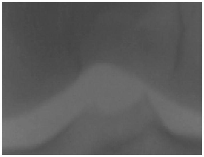
A window of the joint center used for finding the center of the joint in the X-rays

Finding the joint in a given knee X-ray image is performed by first downscaling the image by a factor 10, and then scanning the image with a 15 × 15 shifted window. For each position, the Euclidean distances between the 15 × 15 pixels of the shifted window and each of the 20 15 × 15 pre-defined joint images are computed using Equation 1,

$$d_{i,w}=\sqrt{\sum _{y=1}^{15}\sum _{x=1}^{15}{(I_{x,y}-W_{x,y})}^2}$$ (1)

where W_x,y is the intensity of pixel x, y in the shifted window W, I_x,y is the intensity of pixel x, y in the joint image I, and d_i,w is the Euclidean distance between the joint image I and the 15 × 15 shifted window W.

Since the proposed implementation uses 20 joint images, 20 different distances are computed for each possible position of the shifted window, but only the shortest of the 20 distances is recorded.

After scanning the entire (width/10 – 15) × (height/10 – 15) possible positions, the window that recorded the smallest Euclidean distance is determined as the center of the joint, and the 250 × 200 pixels around this center form an image that is used for the automated analysis. Figure 3 shows an example of the 250 × 200 joint area. Since each image contains exactly one joint, and since the rotational variance of the knees is fairly minimal, this simple and fast method was able to successfully found the joint center in all images in the dataset.

Fig. 3.

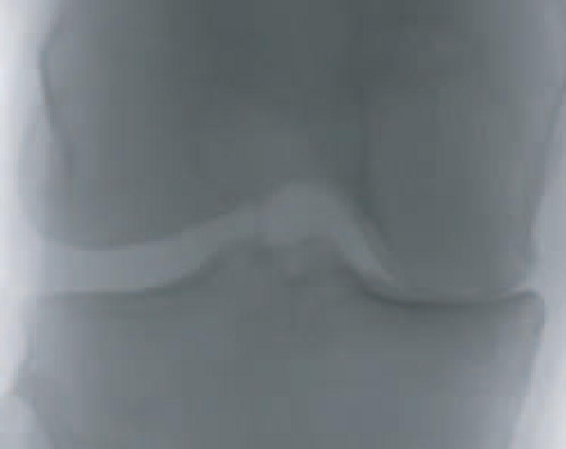
The joint area of a knee X-ray

Using these smaller images for the automated classification keeps them clean from the various background features, and makes the images invariant to the position of the joint within the original X-ray. No attempt is made to fix for the rotational variance of the images, as this small variance is not expected to affect the image analysis described in Section IV, and does not justify automated correction, which can introduce some inaccuracies resulting from the non-trivial task of estimating the exact angle of the joint.

IV. Image Classification

Modern radiography instruments are many times more sensitive than the human eye that observes the resulting images. Therefore, it can be reasonably assumed that OA can be detected by more elements than those proposed by Kellgren-Lawrence, but are not used for the classification due to inability of the human eye to sense them. Since computers are substantially more sensitive to these small intensity variations, an effective use of the strength of computer-based detection would be based on a data-driven classification, rather than an attempt to follow each of the manually classified elements used by Kellgren & Lawrence.

The method works by first extracting a large set of image features, from which the most informative features are then selected. Since image transforms can often provide additional information that is difficult to deduce when analyzing the raw pixels [11], image features are computed not only on the raw pixels, but also on several transforms of the image, and also on transforms of transforms. These image content descriptors extracted from transforms and compound transforms have been found highly effective in classification and similarity measurement of biological and biometric image datasets [11], [25], [26], [28].

For image feature extraction we use the following algorithms, described more thoroughly in [25]:

1. Zernike features [35] are the absolute values of the coefficients of the Zernike polynomial approximation of the image as described in [24], providing 72 image content descriptors.

2. Multi-scale Histograms computed using various number of bins (3, 5, 7, and 9), as proposed by [17], providing 3+5+7+9=24 image content descriptors.

3. First Four Moments of mean, standard deviation, skewness, and kurtosis computed on image “stripes” in four different directions (0, 45, 90, 135 degrees). Each set of stripes is then sampled into a 3-bin histogram, providing 4×4×3=48 image descriptors.

4. Tamura Texture features [34] of contrast, directionality and coarseness, such that the coarseness descriptors are its sum and its 3-bin histogram, providing 1+1+1+3=6 image features.

5. Haralick features [18] computed on the image’s cooccurrence matrix as described in [24], and contribute 28 image descriptor values.

6. Chebyshev Statistics [16] - A 32-bin histogram of a 1 × 400 vector produced by Chebyshev transform of the image with order of N=20.

The image transforms used by the proposed method are the commonly used Wavelet (Symlet 5, level 1) transform, Fourier transform and Chebyshev transform. Additionally, three compound transforms are also used, which are Chebyshev transform followed by Fourier transform, Wavelet transform followed by Fourier transform, and Fourier transform followed by Chebyshev transform. Since human intuition and analysis of image features extracted from transforms and compound transforms is limited, the compound transforms were selected empirically by testing all 2-level permutations of the three basic transforms (Wavelet, Fourier and Chebyshev), and assessing the contribution of the resulting content descriptors to the accuracy of the classification.

Extracting a set of 210 image content descriptors from 7 different image transforms (including the raw pixels) results in a feature vector of dimensionality of 1470. However, not all image features are equally informative, and some of these features are expected to represent noise. In order to select the most informative image features while rejecting the noisy features, each image content descriptor is assigned with a Fisher score [4], described by Equation 2,

$$W_f=\frac{1}{N}{\sum }_{c=1}^N\frac{{(\overline{T_f}-\overline{T_{f,c}})}^2}{{\sigma }_{f,c}^2}$$ (2)

where W_f is the Fisher Score of feature f, N is the total number of classes, $\overline{T_f}$ is the mean of the values of feature f among the images allocated for training, and $\overline{T_{f,c}}$ and ${\sigma }_{f,c}^2$ are the mean and variance of the values of feature f among all training images of class c. The Fisher Score can be conceptualized as the ratio of variance of class means from the pooled mean to the mean of within-class variances. All variances used in the equation are computed after the values of feature f are normalized to the interval [0,1].

Fisher Score values rank the image features by their informativeness, and are assigned to all 1470 features computed by extracting the 210 image content descriptors from the 7 different image transforms (including the original image). Once each of the 1470 image features is assigned with a Fisher score, the weakest 90% of the features (with the lowest Fisher scores) are rejected, resulting in a feature space of 147 image content descriptors. As discussed in Section V, this setting provided the best performance in terms of classification accuracy. The distribution of the different types of image features and image transforms is described in Table II.

TABLE II.

Distribution of the types of features by algorithms and image transforms

Transform	Zernike polynomials	Haralick textures	Tamura textures	First four moments	Multi-scale histogram	Chebyshev statistics	Total
Raw pixels	10	8	1	0	0	6	25
Wavelet	22	1	4	3	0	0	30
Chebyshev	26	0	2	1	2	4	35
Fourier	0	2	2	2	0	0	6
Fourier + Chebyshev	0	10	0	5	7	0	22
Fourier + Wavelet	9	0	1	0	0	4	14
Chebyshev + Fourier	0	10	0	4	1	0	15
Total	67	31	10	15	10	14	147

As the table shows, the most informative image content descriptors are the Zernike polynomials, and both Haralick and Tamura texture features. The radial nature of Zernike polynomials allows these features to reflect variations in the unit disk, so that these features are expected to be sensitive to the joint space in the X-ray images. As observed and throughly discussed by Boniatis et al. [5], the pixel intensity variation patterns mathematically described by the texture features correlate with biochemical, biomechanical and structural alterations of the articular cartilage and the subchondral bone tissues [1], [23]. These processes have been associated with cartilage degeneration in OA [8], [27], and are therefore expected to affect the joint tissues in a fashion that can be sensed by the radiographic texture.

Since not all radiographic elements of OA have been isolated and well-characterized, not all discriminative image features are expected to correspond to a known OA element. Therefore, a small portion of the discriminative values such as the statistical distribution of the pixel values of a Fourier transform followed by a Chebyshev transform is difficult to associate with a known radiographic OA element.

Additional algorithms for extracting image features have been tested, but were found to be less informative for the classification of the KL grades. These image content descriptors include Radon transform features [20], which were expected to correlate with joint space, but were outperformed by Zernike polynomials. Gabor filters [14] captures textural information that could also be useful for the analysis, but were found to be less informative than the Haralick and Tamura textures. Since the areas of interest have relatively low intensity variations, high contrast features such as edge and object statistics as described in [26] do not provide useful information.

After computing all feature values of a given test image, the resulting feature vector is classified using a simple Weighted Nearest Neighbor rule, which is one of the most effective routines for non-parametric classification [4], [36]. The weights, in this case, are the Fisher scores computed by Equation 2. The result of this classification can be a KL grade class determined by the training sample with the shortest distance to the given test sample, but can also be an interpolated value based on the two nearest training samples that do not belong to the same class, as described by Equation 3,

$$KL=(\frac{K_1}{d_1}+\frac{K_2}{d_2})/(\frac{1}{d_1}+\frac{1}{d_2})$$ (3)

where KL is the resulting interpolated KL grade, and d₁, d₂ are the distances from the nearest two samples that belong to different KL grades K₁ and K₂, respectively.

The main advantage of this interpolation is that it can potentially provide a higher-resolution estimation by determining the OA severity within the grade (e.g., KL grade 1.6 for a case of OA severity between KL grade 0 and 1). This, however, is more difficult to evaluate for accuracy since the data used as ground truth only specify the OA severity in resolution of KL grades.

V. Experimental Results

The proposed method was tested using the dataset described in Section II, where the ground truth was the manual classification of the X-rays. In the first experiment, the proposed method was tested by automatically classifying moderate OA (KL grade 3) and normal knees (KL grade 0). The experiment was performed by using 55 X-ray images from each grade, such that 20 images from each grade were used for training and 35 for testing.

This test was repeated 20 times, where each run used a different random split of the training and test images. Since the dataset has more grade 0 images than grade 3, each run used a different set of 55 grade 0 images, randomly selected from the dataset. The classification accuracy was 91.5% (P<0.000001), as can be learned from the confusion matrix of Table III.

TABLE III.

Confusion matrix of of moderate OA and normal

	Normal (KL grade 0)	Moderate OA (KL grade 3)
Normal (KL grade 0)	613	87
Moderate OA (KL grade 3)	32	668

As the confusion matrix shows, the specificity of moderate OA detection is ~86.5%, and the sensitivity is 95%. This can be important for a potential practical use of the described classifier, since it may be over-protective in some cases, but is less likely to dismiss a positive X-ray as normal. It should be noted that while the human readers had a consensus rate of ~80%, the disagreements were usually between neighboring KL grades, and none of the cases had one reader classify a knee as normal while the other classified it as moderate.

Therefore, experienced and knowledgeable readers should be able to tell moderate OA from normal knees with accuracy of practically 100%.

A similar experiment tested the classification accuracy of KL grade 2 (minimal OA). Since this classification problem is more difficult, five more training images were used for each class so that the training set consisted of 25 images of grade 0 and 25 images of grade 2. The use of a larger training set improved the classification accuracy, while increasing the training set in the grade 3 detection did not contribute to the performance, as will be discussed later in this section. The classification accuracy was ~80.4% (P<0.0001), and the confusion matrix is given in Table IV.

TABLE IV.

Confusion matrix of of minimal OA and normal

	Normal (KL grade 0)	Minimal OA (KL grade 2)
Normal (KL grade 0)	222	58
Minimal OA (KL grade 2)	52	228

As can be learned from the table, the specificity of the detection is ~79.3%, with sensitivity of ~81.4%. These numbers show that the detection of KL grade 2 is less effective than the automated detection of KL grade 3. This can be explained by the fact that the progress of OA is continuous, so that KL grade 2 is expected to be visually more similar to 0 than KL grades 3.

We also tried to classify KL grade 1 (doubtful OA) from 0, which provided classification accuracy of 54% when using 25 images per class for training and 14 images for testing. Increaing the size of the training set to 70 samples per class (and 32 samples for testing) marginally increased the performance to 57%. This can be explained by the fact that these two grades are visually very similar, and even experienced human readers often have to struggle to differentiate between the two. Also, since the KL grades are discrete while the actual OA progress is continuous, the very many in-between cases can significantly contribute to the confusion.

Table V shows the classification accuracy when classifying between any pair of KL grades. In all cases, 25 images were used for training, 14 images for testing, and the classification accuracy was computed by averaging the accuracy of 20 random splits to sets of training and test images. Maximum differences from the mean (among the 20 runs) are also specified in the table.

TABLE V.

2-way classification accuracy (%) of all pairs of KL grades

	KL grade 1	KL grade 2	KL grade 3
KL grade 0	54±19	80±8	91±4
KL grade 1		60±13	82±7
KL grade 2	-	-	65±10

As the table shows, classification between two neighboring KL grades is less accurate than classification of non-neighboring grades. We can also see that the two neighboring KL grades 2 and 3 can be differentiated with accuracy of 65%, while the classification of grades 1, 2 and grades 0, 1 provide accuracy of 60% and 54%, respectively. This may indicate that neighboring KL grades are visually more similar to each other in the early stages of OA. It is also noticeable that the classification accuracy improves as the difference between the KL grades gets larger. E.g., the classification accuracy of KL grades 3 and 0 is better than the classification accuracy of KL grades 3 and 1. These results are in agreement with the continuous nature of OA.

Testing the classification accuracy when classifying all 4 KL grades was performed by randomly selecting 25 images from each class for training, and then selecting 14 of the remaining images of each class for testing. This experiment was repeated 20 times, such that in each run the training and test sets were determined in a random manner. The overall classification accuracy of this classifier was 47%, as described by the confusion matrix of Table VI.

TABLE VI.

Confusion matrix of a 4-way classifier of all KL grades

	Grade 0	Grade 1	Grade 2	Grade 3
Grade 0	144	96	21	19
Grade 1	68	60	45	31
Grade 2	10	45	118	107
Grade 3	12	36	105	127

Classification accuracy of 47% may not be considered strong, and it is significantly lower than the 79.8% of agreement between the two human experts. However, the confusion matrix shows that from all cases of KL grade 3, only ~4% were classified as non-OA (KL grade 0), and ~13% as doubtful (KL grade 1). Examining the false positives, the confusion matrix shows that ~7% of the X-rays classified manually as KL grade 0 were falsely classified by the proposed method as KL grade 3 (moderate), and also ~11% of KL grade 1 were mistakenly classified as KL grade 3.

Since the actual OA progress is a continuous variable, there are many in-between cases that can be classified to either of the two closest classes of the given case. E.g., OA progress between KL grade 1 and KL grade 2 can be classified to either 1 and 2. As described in the end of Section IV, the resulting value of the image classification can also be an interpolation of the two nearest KL grades, rather than a single KL grade class. The efficacy of this interpolation can be demonstrated by computing the Pearson correlation coefficient between the predicted and actual KL grades (when using all 4 KL grades as described in Table VI). When using the interpolated value as the predicted grade, Pearson correlation is 0.73, comparing to 0.49 when the predicted KL grade is simply the class of the nearest training sample.

A knee is classified as OA positive if it has been classified as KL grade 2 or higher. By merging the images of KL grades 2 and 3, we introduced a new class called OA positive that contained 78 images (39 from each class). An experiment was performed by building a 2-way classifier using this newly defined class and KL grade 0, such that 60 images from each class were used for training and 18 for testing. The purpose of this experiment was to classify OA positive X-rays from OA negatives. The classification accuracy of this classifier was ~86.1%, with sensitivity and specificity of ~88.7% and ~83.5%, respectively.

It is also important to mention that the X-rays were taken from randomly selected human subjects who participate in the BLSA study, and not necessarily from patients who reported on pain symptoms or were diagnosed as OA positive in one of their other joints. This policy provides a uniform representation of the elderly population, and therefore it can be assumed that the results presented here can be generalized to the entire elderly population.

The classification accuracy may be affected by the size of the training set such that it is expected to increase as the number of training samples gets higher. Figure 4 shows the classification accuracy of the classification of KL grades 2 and 3 from KL grade 0 as a function of the size of the training set. As can be learned from the graph, for KL grade 3 the classification accuracy improves as the size of the training set gets larger, but stabilizes at ~14 training images per class. Classification accuracy of KL grade 2 also increases with the number of training images, but our dataset is not large enough to determine whether it reached the peak of accuracy.

Fig. 4.

Classification accuracy (%) of KL grades 2 and 3 as a function of the size of the training set

As described in Section IV, 10% of the image features with the highest Fisher scores were used for the classification, while the rest of the image content descriptors were ignored. Figure 5 shows how the number of features used for the classification affects the classification accuracy of KL grade 3. According to the graph, the best performance is achieved when using between 7.5% to 12.5% of the total number of image features (1470).

Fig. 5.

Classification accuracy (%) of KL grades 2 and 3 as a function of the number of image features used

In terms of computational complexity, classifying one X-ray image takes 105 seconds, using a system with a 2GHZ Intel processor and 1MB of RAM. While the time required for the joint detection described in Section III is negligible, nearly all of the CPU time is sacrificed for transforming the image and extracting image features. Major contributors to this complexity are the 2-dimensional Zernike features, which are known to be computationally expensive [19], [37]. This downside of the classifier makes it unsuitable for realtime applications or other tasks in which speed is a primary concern, but may be fast enough for classification of single X-ray images, especially considering the fact that the entire procedure of taking X-rays can take a much longer time.

An improvement in the response time of the classifier can be achieved by parallelization of the feature extraction algorithms. Since most of the image features are not dependent on each other, the algorithm becomes trivial to parallelize so that many image features can be computed concurrently by different processors. For instance, while one processor can compute Haralick features on the Chebyshev transform, another processor can extract Haralick features from the Fourier transform, or Zernike features from the Chebyshev transform. In order to take full advantage of the parallelization, the algorithm has been also implemented using the Open Microscopy Environment (OME) software suite [15], [33], which is a platform for storing and processing microscopy images, and designed to optimize the execution and data flow of multiple execution modules. A detailed description of the parallelization of the image transform and image feature extractions in OME can be found in [21].

VI. Conclusion

In this paper we described an automated approach for the detection of OA using knee X-rays. In the absence of an accurate method of OA diagnosis, the manually classified KL grade is used here as a “gold standard”, although it is known that this method is less than perfect. The classification is not performed in a way that attempts to imitate the human classification, but is based on a data-driven approach using manually classified X-rays of different KL grades, representing different stages of OA severity.

Experimental results suggest that more than 95% of moderate OA cases were differentiated accurately from normal cases, with a false positive rate of ~12.5%. Classification accuracy of differentiating minimal OA from normal cases was ~80%, and detection of doubtful OA cases was far less convincing. Future attempts of improving the detection accuracy of doubtful OA will include integrataion of relevant clinical information such as history of knee injury, body weight, and knee alignment angle, and will also use more X-ray samples as they become available. However, due to the subjective nature of the “gold standard”, it is possible that a 100% correlation between computer-based and manual classification may not be achieved. KL grades 4 (severe OA) and 5 (knee replaced) remained outside the scope of this study due to the severe symptoms that accompany these stages, and the relatively easy detection of OA in these stages.

While the classification accuracy of KL grades 1 and 2 cannot be considered strong, it is important to note that radiograph readers are often challenged in attempting to distinguish between these grades, and therefore the confusion of the automated detection between these two grades cannot be considered surprising.

We acknowledge that the equipment used to obtain the knee images does not allow for maximal resolution of joint structures. We speculate conventional radiographic images would predictably allow for better delineation of OA grades, particularly in cases with less severe disease. Certainly conventional radiography is capable of delineating joint structures more readily, but achieves this at the cost of greater radiation exposure. The application of this imaging software to the interpretation of X-ray images occurs without the bias inherent in a clinical interpretation. Finally, this study was conducted within the context of a longitudinal aging study that will enable the comparison of imaging data to clinical OA features as pain, but also to physiologic measures relevant to aging body systems that might contribute to OA severity.

Future plans include testing of this automated technique in the evaluation of longitudinal knee images obtained over time, to check whether OA can be detected before radiographic evidence are noticeable by a human reader. We also plan to develop similar techniques to classify hand X-rays with attention to the signal joints predisposed to the development of OA.

The full source code used for the experiment is available for free download under standard GNU public license via CVS at www.openmicroscopy.org. Scientists and engineers are encouraged to download, compile and use this code for their needs.

Biographies

Lior Shamir is a postdoctoal fellow in the image informatics and computational biology unit, Laboratory of Genetics, National Institute on Aging, National Institutes of Health.

Shari Ling is currently a Staff Clinician in the Clinical Research Branch of the National Institute on Aging Intramural Research Program. She also holds an appointment in the Division of Geriatric Medicine, Gerontology and Rheumatology at Johns Hopkins University School of Medicine, and is on the clinical faculty at the University of Maryland. Her area of interest is aging, osteoarthritis, the identification and development of novel diagnostic and prognostic indicators of arthritis development in the elderly.

William W. Scott Jr. recieved his BA degree in Physical Sciences, magna cum laude, from Harvard University in 1967 and his M.D. degree from the Johns Hopkins University School of Medicine in 1971. He did radiology residency training at Johns Hopkins and was board certified in diagnostic radiology in 1975. Following two years in the USAMC he has worked in radiology at Johns Hopkins where he is Associate Professor of Radiology and was formerly in charge of orthopaedic radiology. For many years he has been one of the radiographic interpreters for the BLSA.

Angelo Bos recieved his M.D. degree from the Fundacao Faculdade Federal de Ciencias Medicas of Porto Alegre, Brazil in 1983, and his Ph.D in Medicine from Tokai University, Kanagawa-ken, Japan. Until 2008 he was senior statistician for the Longitudinal Studies Section at the National Institute on Aging, and now he is an associate professor at the Institute of Geriatrics and Gerontology of Pontifical Catholic University of Rio Grande do Sul, Porto Alegre, Brazil.

Tomasz J. Macura earned his BS degrees, magna cum laude, in Mathematics and Computer Science from the University of Maryland, Baltimore County. He is currently a doctoral candidate at the Computer Laboratory, University of Cambridge, UK (Trinity College) and a Pre-Doctoral Research Trainee at Dr. Ilya Goldberg’s IICBU. His PhD is supported by a National Institutes of Health-University of Cambridge Health Science Scholarship.

Nikita Orlov received his Ph.D. degree in applied mathematics from Moscow State University (Russia) in 1989. He worked as researcher and Sr. researcher in computational electromagnetics laboratory at Moscow University, and then he was with ADE Optical Systems (Charlotte, NC), and ADE Corp. (Norwood, MA). He joined the group of Ilya Goldberg in 2003 (Laboratory of Genetics, NIA), where he works as Sr. research fellow. His interests include pattern recognition, machine vision and biological applications of numerical modeling.

D. Mark Eckley received his BA degree from University of Colorado in 1984, majoring in biochemistry. As a technician at the University of Texas Medical Branch in Galveston, recombinant DNA techniques were mastered, fueling an interest in biology. His MA from University of California, Santa Barbara (1989) had a focus on molecular biology. Training in Cell Biology through the BCMB program at Johns Hopkins School of Medicine led to publication of a thesis, Chromosomal Proteins and Cytokinesis, in 1997. Mark currently works in the Laboratory of Genetics as a Staff Scientist, focusing on microscopy as a genetic screening tool.

Luigi Ferrucci received his medical degree at the University of Florence, where he also earned his doctor of philosophy degree in Biology and Pathophysiology of Aging. Dr. Ferrucci is the Director of the Baltimore Longitudinal Study of Aging and a senior investigator at the Clinical Research Branch of the National Institute on Aging, National Institutes of Health. His research interests involve frailty and mobility disability in the elderly.

Ilya G. Goldberg received his BS in Biochemistry from the University of Wisconsin-Madison in 1990, and his PhD. in Biochemistry and Cell Biology from the Johns Hopkins University School of Medicine in 1997. After a post-doc in crystallography at Harvard, he started the Open Microscopy Environment (OME) project as a post-doc at MIT. In 2002, he returned to Baltimore and joined the Laboratory of Genetics at the National Institute on Aging, where he started a group dedicated to quantitative morphology and systematic functional genomics.

References

- 1.Aigner T, McKenna L. Molecular pathology and pathobiology of osteoarthritic cartilage. CMLS Cell Mol Life Sci. 2002;59:5–18. doi: 10.1007/s00018-002-8400-3. [DOI] [PMC free article] [PubMed] [Google Scholar]
- 2.Altman RD, Gold GE. Atlas of individual radiographic features in osteoarthritis, revised. Osteoarthritis and Cartilage. 2007;15:A1–A56. doi: 10.1016/j.joca.2006.11.009. [DOI] [PubMed] [Google Scholar]
- 3.Ahlback S. Osteoarthrosis of the knee: a radiographic investigation. Acta Radial Suppl. 1968;277:7–72. [PubMed] [Google Scholar]
- 4.Bishop CM. Pattern Recognition and Machine Learning. Springer Press; 2006. [Google Scholar]
- 5.Boniatis I, Costaridou L, Cavouras D, Kalatzis I, Panagiotopoulos E, Panayiotakis G. Osteoarthritis severity of the hip by computer-aided grading of radiographic images. Medical and Biological Engineering and Computing. 2006;44:793–803. doi: 10.1007/s11517-006-0096-3. [DOI] [PubMed] [Google Scholar]
- 6.Boniatis I, Cavouras D, Costaridou L, Kalatzis I, Panagiotopoulos E, Panayiotakis G. Computer-aided grading and quantification of hip osteoarthritis severity employing shape descriptors of radiographic hip joint space. Computers in Biology and Medicine. 2007;37:1786–1795. doi: 10.1016/j.compbiomed.2007.05.005. [DOI] [PubMed] [Google Scholar]
- 7.Browne MA, Gaydeckit PA, Goughll RF, Grennanz DM, Khalilt SI, Mamtoras H. Radiographic, image analysis in the study of bone morphology. Clin phys, Physiol Meas. 1987;8:105–121. doi: 10.1088/0143-0815/8/2/002. [DOI] [PubMed] [Google Scholar]
- 8.Buckwalter A, Mankin HJ. Instructional course lectures, the American Academy of Orthopaedic Surgeons Articular Cartilage. Part II: degeneration and osteoarthrosis, repair, regeneration, and transplantation. Journal of Bone and Joint Surgery. 1997;79:612–632. [Google Scholar]
- 9.Cherukuri M, Stanley RJ, Long R, Antani S, Thoma G. Anterior osteophyte discrimination in lumbar vertebrae using size-invariant features. Computerized Medical Imaging and Graphics. 2004;28:99–108. doi: 10.1016/j.compmedimag.2003.09.002. [DOI] [PubMed] [Google Scholar]
- 10.Croft P. An introduction to the Atlas of Standard Radiographs of Arthritis. Rheumatology Suppl. 2005;4:42. doi: 10.1093/rheumatology/kei051. [DOI] [PubMed] [Google Scholar]
- 11.Gurevich IB, Koryabkina IV. Comparative analysis and classification of features for image models. Pattern Recognition and Image Analysis. 2006;16:265–297. [Google Scholar]
- 12.Kellgren JH, Lawrence JS. Radiologic assessment of osteoarthritis. Ann Rheum Dis. 1957;16:494–501. doi: 10.1136/ard.16.4.494. [DOI] [PMC free article] [PubMed] [Google Scholar]
- 13.Kellgren JH, Jeffrey M, Ball J. Atlas of standard radiographs. Oxford: Blackwell Scientific; 1963. [Google Scholar]
- 14.Gabor D. Theory of communication. Journal of IEEE. 1946;93:429–457. [Google Scholar]
- 15.Goldberg IG, Allan C, Burel JM, Creager D, Falconi A, Hochheiser H, Johnston J, Mellen J, Sorger PK, Swedlow JR. The Open Microscopy Environment (OME) Data Model and XML file: open tools for informatics and quantitative analysis in biological imaging. Genome Biology. 2005;6:R47. doi: 10.1186/gb-2005-6-5-r47. [DOI] [PMC free article] [PubMed] [Google Scholar]
- 16.Gradshtein I, Ryzhik I. Table of integrals, series and products. 5. Academic Press; 1994. [Google Scholar]
- 17.Hadjidementriou E, Grossberg M, Nayar S. Spatial information in multiresolution histograms. IEEE Conf on Computer Vision and Pattern Recognition. 2001;1:702. [Google Scholar]
- 18.Haralick RM, Shanmugam K, Dinstein I. Textural features for image classification. IEEE Trans, on Syst, Man and Cyber. 1973;6:269–285. [Google Scholar]
- 19.Kotoulas L, Andreadis I. Real-Time Computation of Zernike Moments. IEEE Trans, on Circuit, and Systems for Video Technology. 2005;15:801–809. [Google Scholar]
- 20.Lim JS. Two-Dimensional signal and image processing. Prentice Hall. 1990:42–45. [Google Scholar]
- 21.Macura TJ, Shamir L, Johnston J, Creager D, Hocheiser H, Orlov N, Sorger PK, Goldberg IG. Open Microscopy Environment Analysis System: end-to-end software for high content, high throughput imaging. Genome Biology. submitted. [Google Scholar]
- 22.Mengko TL, Wachjudi RG, Suksmono AB, Danudirdjo D. Automated detection of unimpaired joint space for knee osteoarthritis assessment. Proc 7th Intl Workshop on Enterprise Networking and Computing in Healthcare Industry. 2005:400–403. [Google Scholar]
- 23.MartelPelletier J, Pelletier JP. Osteoarthritis: recent developments. Curr Opin Rheumatol. 2003;15:613–615. [Google Scholar]
- 24.Murphy RF, Velliste M, Yao J, Porreca G. Searching online journals for fluorescence microscopy images depicting protein subcellular location patterns. Proc 2nd IEEE Intl Symp on Bioinformatics and Biomedical Eng. 2001:119–128. [Google Scholar]
- 25.Orlov N, Johnston J, Macura T, Shamir L, Goldberg I. Computer Vision for Microscopy Applications. In: Obinata G, Dutta A, editors. Vision Systems. Advanced Robotic Systems Pub.; Vienna, Austria: 2007. pp. 221–242. [Google Scholar]
- 26.Orlov N, Shamir L, Macura T, Johnston J, Eckely DM, Goldberg I. WND-CHARM: Multi-purpose image classification using compound image transforms,". Pattern Recognition Letters. 2008;29:1684–1693. doi: 10.1016/j.patrec.2008.04.013. [DOI] [PMC free article] [PubMed] [Google Scholar]
- 27.Radin EL, Rose RM. Role of subchondral bone in the initiation and progression of cartilage damage. Clin Orihop. 1986;213:34–40. [PubMed] [Google Scholar]
- 28.Rodenacker K, Bengtsson E. A feature set for cytometry on digitized microscopic images. Anal Cell Pathol. 2006;25:1–36. doi: 10.1155/2003/548678. [DOI] [PMC free article] [PubMed] [Google Scholar]
- 29.St Clair SF, Higuera C, Krebs V, Tadross NA, Dumpe J, Barsoum WK. Hip and knee arthroplasty in the geriatric population. Clin Geriatr Med. 2006;3:515–533. doi: 10.1016/j.cger.2006.04.004. [DOI] [PubMed] [Google Scholar]
- 30.Shock NW, Greulich RC, Andres R, et al. Normal human aging: the Baltimore Longitudinal Study of Aging. Washington, DC: Government Printing Office; 1984. NTH Publication No. 84–2450. [Google Scholar]
- 31.Stockwell RA. Cartilage failure in osteoarthritis: relevance of normal structure and function - A review. Clin Anat. 1990;4:161–191. [Google Scholar]
- 32.Sun Y, Gunther KP, Brenner H. Reliability of radiographic grading of osteoarthritis of the hip and knee. Scandinavian Journal of Rheumatol. 1997;26:155–165. doi: 10.3109/03009749709065675. [DOI] [PubMed] [Google Scholar]
- 33.Swedlow JR, Goldberg I, Brauner E, Sorger PK. Informatics and quantitative analysis in biological imaging. Science. 2003;300:100–102. doi: 10.1126/science.1082602. [DOI] [PMC free article] [PubMed] [Google Scholar]
- 34.Tamura H, Mori S, Yamavaki T. Textural features corresponding to visual perception. IEEE Trans, on Syst, Man and Cyber. 1978;8:460–472. [Google Scholar]
- 35.Teague MR. Image analysis via the general theory of moments. Journal of the Optical Society of America. 1979;70:920–920. [Google Scholar]
- 36.Theodoridis S, Koutroumbas K. Pattern Recognition. 2. Elsevier Academic Press; 2003. [Google Scholar]
- 37.Wee CY, Paramesran P. Efficient computation of radial moment functions using symmetrical property. Pattern Recognition. 2006;39:2036–2046. [Google Scholar]