Selective Genotyping and Phenotyping Strategies in a Complex Trait Context

Abstract

Selective genotyping and phenotyping strategies are used to lower the cost of quantitative trait locus studies. Their efficiency has been studied primarily in simplified contexts—when a single locus contributes to the phenotype, and when the residual error (phenotype conditional on the genotype) is normally distributed. It is unclear how these strategies will perform in the context of complex traits where multiple loci, possibly linked or epistatic, may contribute to the trait. We also do not know what genotyping strategies should be used for nonnormally distributed phenotypes. For time-to-event phenotypes there is the additional question of choosing follow-up time duration. We use an information perspective to examine these experimental design issues in the broader context of complex traits and make recommendations on their use.

QUANTITATIVE trait locus (QTL) experiments provide valuable clues for identifying genetic elements responsible for quantitative trait variation (Lander and Botstein 1989; Lynch and Walsh 1998; Rapp 2000). For best results, QTL experiments require that large numbers of individuals be genotyped and phenotyped for the quantitative trait of interest. Since this can be a costly endeavor, investigators employ cost-saving strategies such as selective genotyping, in which a selected portion of the phenotyped individuals are genotyped (Lebowitz et al. 1987; Lander and Botstein 1989; Darvasi and Soller 1992), and selective phenotyping, in which a selected portion of the genotyped individuals are phenotyped (Jin et al. 2004). The efficacy of these strategies has been evaluated in simplified settings where a single locus contributes to the phenotype and when the phenotype (conditional on genotype) is normally distributed. It is therefore unclear how effective these strategies would be in the broader context of complex trait genetic analyses. In such settings, we suspect that multiple loci, possibly linked and epistatic, contribute to the trait, and the trait distribution may be nonnormal.

The value of selective genotyping has also been recognized in human association studies and is currently being actively researched (Chen et al. 2005; Wallace et al. 2006; Huang and Lin 2007). Interest in this application is primarily motivated by the fact that these studies require dense high-throughput genotyping, which can be expensive. However, similar to QTL studies in experimental crosses, the theoretical results have focused primarily on normally distributed phenotypes and single-locus models.

Sen et al. (2005) examined the effectiveness of selective genotyping when two unlinked additive QTL contribute to a normally distributed trait. Because epistasis appears to be a common and important feature of many complex traits (Frankel and Schork 1996), it is important to investigate whether epistasis can also be detected in selectively genotyped samples. Experimental studies appear to be divided over this issue. Some studies have reported epistasis in selectively genotyped samples (Ohno et al. 2000; Abasht and Lamont 2007) while others failed to detect it (Carr et al. 2006), citing concerns about loss of power. Thus, the generality of these experimental observations requires further theoretical exploration.

In the context of association studies, Gallais et al. (2007) compared one-tail and two-tail selective genotyping and showed that the latter is superior. However, many interesting traits are nonnormally distributed. Time-to-event phenotypes, such as survival times or tumor onset, are important cases when the trait is expected to be nonnormally distributed, usually with a long right tail. In these situations, individuals in the right tail are likely to be genetically more informative, and it is unclear which type of selection strategy (one-tail, two-tail, or a different strategy) should be applied. Moreover, from a cost-saving perspective the additional problem arises that the most informative individuals (those in the right tail) will also be the most expensive to phenotype because of the cost of following the individuals until the event of interest has been observed. The investigator must therefore decide to either stop following up, which results in reduced cost and a loss of information due to censoring, or follow up the entire sample until all events have been observed, which implies greater cost but a minimal loss of information. As far as we are aware, these trade-offs have not been studied.

In studies where phenotyping is more expensive than genotyping, Jin et al. (2004) proposed selective phenotyping. Here individuals selected for phenotyping have maximal genetic diversity in a genomic region of interest. Their simulations showed that for a fixed number of phenotyped individuals, this approach increases power relative to a random sample. Although this gain in power diminishes when multiple genomic regions are considered, it outperforms phenotyping a random sample. Selective phenotyping is particularly attractive for genetical genomics studies (Jansen and Nap 2001) where the traits of interest consist of thousands of genomewide molecular measurements (e.g., transcriptome, metabolome, proteome) obtained using high-throughput technologies such as microarrays and mass spectrometry. For studies using two-color microarrays, Fu and Jansen (2006) proposed a related selective phenotyping strategy that increases power by cohybridizing mRNA from genetically distant pairs of individuals onto the same array.

The above-mentioned experimental design problems have one common feature—they involve experimental strategies (selective genotyping, selective phenotyping, choice of follow-up period) that trade off information and experimental cost. Sen et al. (2005) showed that by adopting an information perspective, one can formally study these trade-offs in QTL studies. In this article we use the information perspective to explore the following issues: (a) How does selective genotyping perform when multiple loci contribute to the phenotype?, (b) How does selective phenotyping perform when multiple loci are used for selection?, (c) How should selective genotyping proceed if the trait is not normally distributed?, (d) What selective genotyping approach is appropriate for lifetimes?, (e) How should we choose the duration of follow-up?, and (f) How should we combine selective genotyping with choice of follow-up duration?

Our article is organized as follows. In the next section we review the theory underlying our information perspective. In the following section we present the results obtained by applying that theory to answer each of the six questions posed in the previous paragraph. We conclude with a discussion of our results.

THEORY

Information perspective on QTL study design:

Traditionally, the efficacy of QTL study designs has been investigated using power calculations. In the experimental design literature, notably industrial experimental design, study designs are evaluated using their information matrix. The information matrix is a fundamental statistical quantity; the power of a study design, the expected LOD score (which is a log-likelihood ratio), and variance of estimated QTL effects all depend on the information matrix. The expected Fisher information is defined as the expected value of the second derivative of the log-likelihood function,

where ℓ(β | y_obs) denotes the log-likelihood function for the parameter of interest β, when the observed data are y_obs. For large sample sizes, the variance of the maximum-likelihood estimate, is

The log-likelihood ratio statistic for testing β = β₀ is

which, for large samples, has an approximate noncentral χ²-distribution with s (dimension of β) degrees of freedom and noncentrality parameter (β − β₀)′J(β)(β − β₀). The log-likelihood ratio expressed in base 10 logarithms is the LOD score. Thus, the power of the likelihood-ratio test, which depends on the noncentrality parameter, depends on the unknown state of nature (β − β₀) and the information matrix, J(β). The experimenter has no control over the state of nature, but has limited control over experimental design choices that determine the information content. Thus the information content of a study design provides us with a parsimonious description of the statistical characteristics of the study.

Criteria for evaluating designs:

We calculate the expected Fisher information (for the QTL effect parameters conditional on QTL location) for each genotyping strategy in each context. This is used to evaluate the usefulness of selective genotyping in each genetic model context. When multiple loci are involved, the information is a matrix, and we have to resort to one-dimensional summaries of the information matrix.

In the experimental design literature, a few different summary measures (optimality criteria) have been proposed for comparing alternative designs (Cox and Reid 2000). We compare the designs here using two criteria based on the information matrix J, or equivalently V = J⁻¹:

1. D-optimality criterion: This criterion maximizes the determinant of the information matrix, det(J), or equivalently (det(J))^1/k, where k is the number of parameters. It minimizes the volume of the joint confidence ellipsoid of all the parameters. It is the most popular design criterion because it makes full use of the information matrix and is not affected by orthogonal reparameterizations of the parameter.

2. c-optimality criterion: This criterion maximizes the inverse of the variance of a contrast c between model parameters, (c′Vc)⁻¹.

The appropriate criterion depends on one's objective. In this article, we use the c-optimality and D-optimality criteria.

Calculation of the information content:

We use missing data methods to calculate the expected information content under selective genotyping. When we use selective genotyping, we deliberately choose not to collect genotyped data on certain individuals on the basis of their phenotype. These data are missing data. We use the missing data principle to calculate the expected information content of any genotyping strategy. The missing information principle (Orchard and Woodbury 1972; McLachlan and Krishnan 1996) states that the observed information, I_o, may be calculated as

where the observed information is

the missing information is

and the complete information is

In the selective genotyping context, y_obs consists of the phenotypes and the genotypes of genotyped individuals. The missing data, y_mis consist of the genotypes at all ungenotyped locations. Since the expected information satisfies J(β) = E(I_o(β)), we can use the missing information principle to calculate the expected information content of genotyping designs.

Backcross population, single-locus model:

Assume we have a population of n individuals. Let y denote the phenotype of an individual and let g denote the genotype at a particular locus. Let β denote the genetic model parameters. In general, β is a vector. The phenotype is assumed to be normally distributed given the QTL genotypes with mean depending on β and variance 1.

Assume that a single locus contributes to the trait variation, and consider a single individual with phenotype y and with q denoting the conditional probability that the individual is homozygous at a locus, given the available marker data. Sen et al. (2005) showed that, in this case, the contribution of the individual to the observed information is

where q*/(1 − q*) = e^2βq/(1 − q). At a locus with no nearby markers genotyped, q = , so that the observed information is

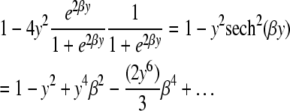If the individual is genotyped, then the observed information is simply 1. When selectively genotyping with selection fraction α, we genotype an α-fraction of the most extreme phenotypic individuals. Thus, if z(α, β) is the upper α-point of the phenotype distribution when the QTL effect is β, then the expected information using the two-tail selective genotyping strategy is

For small β,

where z_α is the upper α-point of the standard normal distribution.

The observed information corresponding to an individual phenotype y gives an indication of the value of genotyping that individual. Integrating over the observed information corresponding to a genotyping strategy, we can get the expected information resulting from that genotyping strategy. Thus, we can devise and evaluate strategies by examining the observed information and the expected information.

Backcross population, two unlinked loci:

Let g₁ and g₂ denote the QTL genotypes at two unlinked loci. Assuming that the two loci are additive, we can write the genetic model for the phenotype as

(1)

where β₀ is the overall mean, β₁ and β₂ are the effects of the first and second QTL, respectively, and ɛ is the random error that is normally distributed. For simplicity, we assume β₀ = 0 for the rest of this article. Sen et al. (2005) used the above-mentioned approach to calculate the expected information for β = (β₁, β₂), when β₁ = 0, and β₂ = β. This gives us the missing information when the first QTL has small effect as a function of the effect of the second QTL. In this setting the missing information matrix for an ungenotyped individual with phenotype y was shown to be

Note that when the second QTL has a small effect, the expected information under selective genotyping behaves similarly as with a single QTL. As the strength of the second QTL the information content for the first QTL progressively decreases. The worst scenario is when the second QTL has a really dramatic effect. In this setting, when half the extreme individuals are genotyped, only half the information is obtained—this is the same as genotyping randomly selected individuals (random genotyping). When more than half of the extreme individuals are genotyped, selective genotyping performs worse than random genotyping.

RESULTS

How does selective genotyping perform when multiple loci contribute to the phenotype?

In this subsection we examine the efficacy of selective genotyping when multiple loci contribute to phenotypic variation. In the interests of simplicity, we consider backcross populations and normally distributed residual variation. We begin by examining the case of two linked loci acting additively. Next, we consider two unlinked epistatic loci contributing to the trait.

Two linked loci:

Let g₁ and g₂ denote the QTL genotypes at two loci separated by a recombination fraction θ. Our objective is to evaluate the expected information content of a selective genotyping design where α-fraction of the extreme phenotypic individuals are genotyped. Assume that the QTL act additively; i.e., the genetic model for the phenotypes is the same as (1). First note that with complete genotyping, the expected information matrix per observation is

Thus, det(J) = 4θ(1 − θ). The variance of the parameter estimates is thus

Using either a D-optimality criterion (the determinant of the information matrix) or the inverse of the variance of the first locus effect, , we see that the information for two linked loci is a function of θ(1 − θ), which is maximum when the two loci are unlinked and gets progressively smaller as θ approaches 0.

Our goal is to examine how selective genotyping affects the information to detect two linked loci. To do this, we calculate the information matrix using the missing information principle. The missing information matrix is

Note that when the QTL are unlinked, i.e., , the missing information for β₁ is

which coincides with the result for unlinked loci derived earlier. Further,

where A = y²sech²(βy), and . Thus,

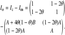Therefore the expected information has the form

where , and ; the integral is with respect to the marginal distribution of y (which depends on β) and over the range of y for which genotyping is not performed (determined by the selection fraction, α). Note that A, A*, B, and B* are independent of θ. Since the information is not scalar, we use two scalar summaries, the determinant and the inverse of the variance of the , to evaluate the impact of selective genotyping and linkage (measured by θ). First, note that the determinant of the information matrix

is a product of terms that involve θ and those that depend on α and β. This implies that by the D-optimality criterion, the effect of selective genotyping and linkage of the two loci are independent. Thus, beyond the loss of information due to linked loci, the effect of selective genotyping is exactly as for unlinked loci. Next, note that the variance matrix is

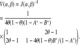Here also, the variance of is the product of two terms, one that depends on how linked the loci are and another that depends on the selective genotyping scheme. This implies that the effect of selective genotyping on the detection of a locus with small effect in the presence of a linked locus is independent of the extent of linkage.

Two epistatic loci:

We analyze the case of two epistatic loci with the same approach as for two linked loci. Consider the following linear model for the phenotype,

(2)

where β₃ is the epistatic effect of the two QTL. We consider two important special cases when the epistatic effect is small: (a) when there is one major main effect and the other locus has a small effect (β₁ = β, β₂ = 0, β₃ = 0) and (b) when both loci have equal but nonzero main effects (β₁ = β, β₂ = β, β₃ = 0). The analytic expressions for the observed information matrix are included in the supplemental information. We graph the functions in Figures 1 and 2.

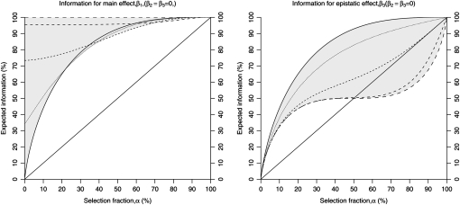
Figure 1.—

Expected information in a two-QTL model with epistasis, as a function of the selection fraction α for main effects (β₁, left) and epistatic effects (β₃, right). The information is plotted as we vary the size of the main effect of the first QTL, while the second QTL and epistatic effect size is assumed to be zero. The shaded region is the space of variation as β₁ varies from 0 to ∞. The solid line corresponds to β₁ = 0, and successive dashed lines (as the size of the dash increases) correspond to the proportion of variance explained by the first QTL equal to 20, 50, 75, and 90%. If the proportion of variance explained by the main-effect QTL is <20%, the expected information is approximately equal to that when the proportion variance explained is 0%. Information for the main effect increases as the size of the effect increases. The information for the epistatic effect decreases as the size of the main effect increases. For selection fractions >50% selective genotyping may be less efficient than even random sampling (solid diagonal line), for which the expected information is equal to the selection fraction. This is specially so when the variance explained by the main effect exceeds 50%.

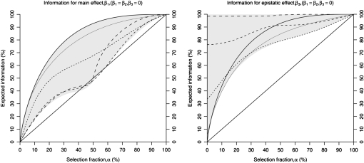
Figure 2.—

Expected information in a two-QTL model with epistasis, as a function of the selection fraction α main effects (β₁, left) and epistatic effects (β₃, right). The information is plotted as we vary the size of the main effects of both QTL, assumed to be of equal effect, while the epistatic effect size is assumed to be zero. The shaded region is the space of variation as β₁ varies from 0 to ∞. The solid line corresponds to β₁ = β₂ = 0, and successive dashed lines (as the size of the dash increases) correspond to the proportion of variance explained by the main-effect QTL equal to 20, 50, 75, and 90%. The diagonal solid line is the efficiency of genotyping a random subset. If the proportion of variance explained by the main-effect QTL is <20%, the expected information is slightly less than that when the proportion of variance explained is 0%. Information for the main effects decreases as the size of the effects increases, but the pattern is not monotonic with the effect size. The information for the epistatic effect approaches 100% as the size of the main effects increases. This “hyperefficiency” relative to when the main effect size is zero is most pronounced when the proportion of variance explained by the main effects exceeds 75%.

We find that as long as the proportion of variance explained by the main-effect QTL remains <20%, the effectiveness of selective genotyping is approximately the same as that for the case when a single locus with a main effect is segregating in the cross. When the proportion of variance explained by the main-effect QTL is larger, the efficiency of selective genotyping for detecting epistasis varies. In some cases, it can be less efficient than random sampling (Figure 1); in other cases it may have more information than that for the main-effect loci (Figure 2).

How generalizable are these results to F₂ intercross and SNP association studies?

In our results above, we confined our explorations to the backcross, for simplicity. In this section, we present simulation studies to explore the generality of the conclusions to SNP association studies and F₂ intercross.

We generated data using the model

(3)

where x_i = g_i − 1, and g_i is an allele count at the ith locus (0, 1, or 2). Then we analyzed an α-fraction of the extreme phenotypic individuals in the manner of a case–control study. We defined a new variable z as 0/1, indicating the bottom α/2 phenotypic individuals (“control”) and the top α/2 fraction (“case”). Then we analyzed the data using logistic regression of z on the x's, as in a case–control genetic study, using the three-QTL model above. We calculated the P-values of the regression coefficients. We then compared the results of that analysis to that when the data are generated from the same model, but with only one nonzero term. This allows us to compare the effect of other QTL on the detection of the effect. We varied the effect sizes (the β's), the sample size, the selection fraction α, and the allele frequencies. In Table 1 we present the results from two batches of simulations where we varied the main effect of a locus and the allele frequencies for α = 0.2. If the proportion of the variance explained by the largest locus is ≤10%, then the power is approximately the same. Power losses are appreciable once the proportion variance explained by the locus with the largest effect approaches 20%. We conducted other simulations (not shown) with other parameter configurations that broadly give the same message; the reader is invited to explore other parameter values using our software code (presented in the supplemental information).

TABLE 1.

Power to detect main-effect and interactive loci in a SNP association study using selective genotyping in the context of a three-QTL model, using a selection fraction (α = 20%), and treating the selectively genotyped sample as a case–control study (see text for details)

		Power (%)
Three-QTL model				Single-term model
Parameters	β1 (% QTL variance)	β1	β2	β3	β12	β1	β2	β3	β12
r = 0.5; n = 800	0.1 (0.5)	96	55	78	78	96	52	79	80
	0.2 (2.0)	100	53	75	75	100	56	77	79
	0.4 (8.0)	100	50	72	66	100	53	80	78
	0.6 (18.0)	100	43	67	49	100	51	78	80
	0.8 (32.0)	100	37	58	34	100	52	77	82
r = 0.8; n = 2500	0.1 (0.3)	96	51	96	85	97	50	96	88
	0.2 (1.3)	100	48	97	82	100	54	97	88
	0.4 (5.1)	100	42	93	74	100	55	97	86
	0.6 (11.5)	100	33	92	62	100	54	97	86
	0.8 (20.5)	100	28	87	57	100	56	96	87

The power corresponds to tests with a significance level of 0.10. It was estimated using 10,000 simulations, and the estimates are correct to ±1%. In the simulations, β₀ = 0, β₂ = 0.05, β₃ = 0.07, and β₁₂ = 0.1; n is the sample size of the “case–control” sample; the actual sample size is 5n. We denote by r the common major allele frequency for the loci. The power to detect the main-effect β₁ increases with β₁, as expected, but the power to detect other loci and the interaction term (β₂, β₃, and β₁₂) decreases with β₁. The decrease in power is most severe when the variance explained by the strongest locus exceeds 10%.

How does selective phenotyping perform when multiple loci are used for selection?

Jin et al. (2004) proposed selective phenotyping as a cost-saving measure when phenotyping is substantially more expensive than genotyping. In this section we analyze the effect of selection based on multiple unlinked regions on the information content of the experiment.

The idea underlying selective phenotyping is to pick a subset of individuals who are as genetically diverse as possible at given candidate regions. The efficiency of this approach decreases as the number of unlinked loci considered increases. To motivate the general result we first consider a single locus, then two unlinked loci, and then the general case. Throughout we consider selective phenotyping in an F₂ population where genotypes at any given locus are coded 0, 1, and 2 corresponding to the number of alleles from a particular inbred strain. We focus on detecting the additive effect of a locus.

Single locus:

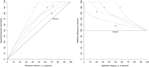
The most efficient strategy is to first pick equal numbers of the two homozygotes (corresponding to genotypes 0 and 2) until they are exhausted. Then we pick the heterozygotes (corresponding to the genotype 1). Note that for detecting additive effects, heterozygotes are not informative, so on average, just studying half the population is as effective as studying all of it. This is reflected in Figure 3.

Figure 3.—

Information of selective phenotyping as a function of the selection fraction and the number of unlinked genetic loci used for selection. The left panel shows the expected information from selected phenotyping as a function of the selection fraction when 1, 2, 3, or 10 loci are used for selection. The solid line shows the expected information from random sampling. The right panel shows the information from selective phenotyping relative to random sampling as a function of the selection fraction. We see that as the number of loci increases, the efficiency of selective phenotyping approaches random selection. However, the relative efficiency for small selection fractions can be quite high even when 10 loci are used for selection.

Suppose we select an α-proportion of the sample for phenotyping, and of those a proportion τ are homozygotes. Then it is easily seen that the information content of the sample relative to studying the full sample is 2τα. We use this result for proving the general result for an arbitrary number of loci.

Two loci:

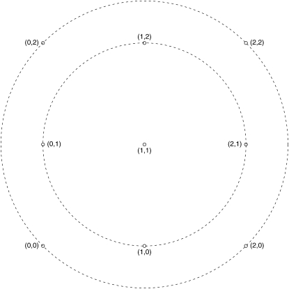
When selective phenotyping is performed using two loci, the genotypes can be represented as in Figure 4. There are three genotype classes depending on the number of homozygous loci (zero, one, or two). These correspond to the center point, the inner circle, and the outer circle, respectively. The outer circle genotypes are the most different and represent the greatest genetic diversity, followed by the inner circle, and finally the center point. Thus, the optimal strategy is to first select equal numbers of individuals from the outer circle (two homozygous loci), then the inner circle (one homozygous locus), and finally the center point (zero homozygous loci). The outer circle covers one-quarter of the sample, the inner circle one-half, and the center point one-quarter.

Figure 4.—

Distances of genotypes from the average genotype for two-locus genotypes in an F₂ intercross. We code genotypes at each locus as 0, 1, or 2. The x-axis and the y-axis are used to plot the genotypes at the first and second locus, respectively. The average genotype is the (1, 1) genotype (double heterozygote) at the center. Two concentric circles are drawn to depict two sets of equidistant points from the center. The outermost circle consists of the homozygous genotypes, the points (0, 0), (0, 2), (2, 2), and (2, 0). These are the points most distant from the center. The inner circle consists of genotypes homozygous at one locus and heterozygous at the other, the points (0, 1), (1, 2), (2, 1), and (1, 0). These are the next most distant from the center. To pick the most genotypically diverse individuals, one would first pick individuals with genotypes in the outermost circle, then the inner circle, and finally the center.

If the loci considered are unlinked, the effect estimates corresponding to the loci are uncorrelated with each other and, hence, orthogonal. Thus, using symmetry, the information content of the whole sample can be evaluated through the information of any single locus.

Let us consider the information content corresponding to three key α-values: , when the outer circle points are included; , when the outer and inner circle points are included; and 1, when all points are included. When α = , at any given locus all individuals are homozygous. Thus, the information content is . When α = , all homozygous individuals are in the sample; they compose two-thirds of the selected sample. Thus, the information content is . When α = 1, all individuals are in the sample, and thus the information content is 1. The information content of all other α-values can be calculated by linear interpolation as in Figure 3.

Arbitrary number of loci:

We can now tackle the general case with m unlinked loci, where the genotypes can be represented as points on a lattice in an m-dimensional space. There are m + 1 classes of points corresponding to their distance from the center point, representing an individual heterozygous at all loci. The classes are defined by the number of homozygous loci, 0–m. The proportion of the sample in each of these classes is given by the probability mass function of a binomial distribution with parameters m and . The expected information content of the class with k homozygous loci is

Thus, the information content of a sample that has chosen the classes m, m − 1, …, k is

The information content corresponding to intermediate selection fractions can be found by linear interpolation. The function info.pheno in the R/qtlDesign package (Sen et al. 2007) calculates the information content of selective phenotyping.

We find that as the number of loci used for selective phenotyping increases, the efficiency of selective phenotyping decreases. In the limit, it reduces to random selection. However, it is notable that the gain in efficiency relative to random selection is higher for small selection fractions (the fraction of individuals selected for selective phenotyping). In other words, if phenotyping is very expensive relative to genotyping and rearing, then even if a large number of loci (or the whole genome) are used for selective phenotyping, it will be effective. These findings are consistent with the simulation studies of Jin et al. (2004) and provide a theoretical justification for their observations.

How should selective genotyping proceed if the trait is not normally distributed?

The logic of selective genotyping is that extreme phenotypic individuals provide the most information. This may not hold for all situations. For example, if the phenotype is heavy-tailed, the most extreme individuals are less informative. In other words, we expect individuals with moderately high, but not the most extreme phenotypes, to be the most informative. This argument implicitly assumed that both extremes of the phenotype are equally important. For lifetime distributions, it is reasonable to expect that the right tail is more important than the left tail, but this asymmetry is not reflected in two-tailed selective genotyping strategies. To help us choose a genotyping strategy on the basis of the nature of the phenotype distribution, we develop the idea of the information gain function below.

Information gain function:

We develop our ideas in the context of a backcross. Let y be the phenotype of an individual, g = 0, 1 be the QTL genotype at a locus of interest, and q = P(g = 1 | m) be the probability of the 1 genotype given the marker genotype information, m. Let the distribution of the phenotype given the QTL genotype be p(y | g). The observed data consist of (y, m), while the missing data are g. We want to know, on the basis of an individual's phenotype, how informative that individual will be. Let p(y | g = 0) = f(y, −δ) and p(y | g = 1) = f(y, +δ), where f is the phenotype density. In our context, the missing data are the unobserved QTL genotypes, and the observed data consist of the marker genotypes and the phenotypes. The parameter of interest is δ. Thus the distribution of the missing data conditional on the observed data is q*^g(1 − q*)^1−g, where q* = P(g = 1 | y, m, δ). Since q = P(g = 1 | m), by Bayes theorem it is easy to see that

Hence the missing data log likelihood is

Differentiating twice, we get

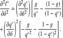Hence,

where

is a function depending on the phenotype density f. We expect this function to change with the shape of the phenotype distribution. By calculating this function, which we call the information gain function, for different functional forms of f, we can identify the individuals that are best to genotype. We use Taylor expansions for small δ, the most interesting scenario. For the normal distribution, h(y, q, δ) = y² and captures the fact that most information is to be gained from the extremes of the distribution. Information gain functions for selected distributions are shown in Table 2.

TABLE 2.

The density function and the information gain function for select distributions

Distribution	Density function	Information gain	Expected information	Parameter
Normal		y2		θ
Cauchy				θ
Logistic				θ
Exponential	(1/σ) exp(−y/σ), y > 0	4(y − 1)2	α + α log(α)2	θ = log(σ)
Gamma		4(y − ν)2		θ = log(σ)
Weibull	(ν/σ) (y/σ)ν−1 exp(−(y/σ)ν), y > 0	4ν2(yν − 1)2	α + α log(α)2	θ = log(σ)

The parameter of interest for the first three distributions is the location parameter. For the last three, the parameter of interest is the scale parameter, the respective shape parameters being fixed. ψ(·, ·) is the incomplete Gamma function.

Location shift—symmetric distributions:

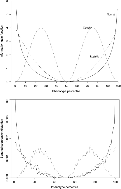
We first examine symmetric distributions with a location shift depending on genotype. Our calculations show very different information gain functions for the normal and Cauchy distributions (Figure 5). This suggests that the most extreme phenotypic individuals are not as informative when the phenotype distribution is Cauchy, as it is when the phenotype distribution is normal.

Figure 5.—

Top: Plot of the information gain function against the phenotype percentile for normal, Cauchy, and logistic distributions. We see that the extreme phenotypic individuals are very informative if the phenotype has a normal or logistic distribution. However, if the phenotype follows a Cauchy distribution, the extreme phenotypic individuals are not very informative. The most informative individuals are those near the first and third quartiles. Bottom: Plot of the squared deviation of the segregation ratio from the expected 50% by percentile of phenotype distribution from 10,000,000 simulations. The squared segregation ratios conditional on phenotype have shapes similar to the information gain function.

To study this further, we conducted a simulation study as follows. We simulated 10,000,000 individuals from a backcross. Conditional on the genotype, the phenotype in the two genotype groups was location shifted by 0.1 times the interquartile range (IQR). Then we examined the genotype ratios conditional on the percentile of the phenotype distribution. Uninformative percentiles would be those where the genotype ratio is 0.5. The further the deviation from 0.5, the more informative the percentile. Assuming that the two genotypes are coded 0 and 1, let p_q be the proportion of 1 genotypes conditional on the phenotype y being in the qth percentile. We plot (p_q − 0.5)² as a function of q to see which percentiles most discriminate between the two genotypes (Figure 5).

The simulation study confirmed what the information gain function suggests: the most extreme individuals are most informative when the phenotype distribution is normal or logistic; however, they are not the most informative if the phenotype has a Cauchy distribution. This shows that the best selective genotyping strategy depends on the shape of the phenotype distribution and that the traditional two-tail selective genotyping strategy is not always the best. We explore this further by examining the information gain function for typical survival distributions.

Scale shift—lifetime distributions:

For lifetime distributions we focused on the exponential distribution and two families extending it: the Gamma and Weibull distributions. We calculated the information gain function for a scale shift (supplemental Figure 1) and found that the upper tail, containing individuals with the longest lifetimes (top 15%), is more informative than the shortest-lived individuals. This suggests that for phenotypes with a long right tail we should selectively genotype by oversampling the right tail. Although the information gain functions for Weibull and exponential distributions appear different in functional form (Table 2), they are identical as a function of phenotype percentile.

As with the symmetric distributions we simulated 10,000,000 individuals from a backcross. Conditional on the genotype, the scale parameter of the phenotype in the two genotype groups was shifted by 10%. We examined the genotype ratios conditional on the phenotype percentile (supplemental Figure 1). As with the symmetric distributions, the shape of the information gain function paralleled that of the squared deviation of the segegation ratios from 1/2.

Thus, the information gain function, which we defined on theoretical considerations, shows us which individuals' genotypes are most likely to deviate from the average genotype. It can therefore be used to prioritize individuals for selective genotyping.

What selective genotyping approach is appropriate for lifetimes?

Since the right tail is more informative for phenotypes with a long right tail such as lifetimes, we investigate single-tail selective genotyping, where individuals with the longest lifetimes are genotyped. We concentrate on the exponential distribution, which has a central role in the analysis of lifetimes (and time-to-event data). The expected information for small-effect sizes as a function of the selection fraction, α, has a simple form:

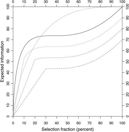
Comparing this with the expected information from traditional two-tail selective genotyping for normally distributed phenotypes (Figure 6) reveals important differences. Although the expected information rises more steeply for small α, it flattens out for α between 20 and 70%. This is because after ∼20% of the individuals have been genotyped, one-tail genotyping is no longer the most efficient strategy (as indicated by the information gain function); the best strategy is to genotype both tails after that point. Nevertheless, a one-tail genotyping strategy is simpler to implement in practice.

Figure 6.—

Expected information for single-tail selective genotyping as a function of the selection fraction, and proportion censored. We assume that the trait distribution is exponential and that the effect size affecting the scale parameter is small. We assume that all individuals until a certain time are followed up and the rest are censored. The solid black line shows the expected information for an exponential information with no censoring (100% follow-up). The dashed lines with increasing dash size show, respectively, the expected information with 10, 20, and 30% censoring. The solid gray line shows, for reference, the expected information for a normal distribution with two-tail selective genotyping. With no censoring, genotyping 20% of the longest-lived individuals gives us almost 75% of the information. However, the gains from selective genotyping more individuals are modest thereafter.

Next we consider the impact of genotyping cost on selective genotyping. As in Sen et al. (2005) we consider a simple linear cost function. Let c be the cost of genotyping relative to raising and phenotyping an individual. Our goal is to maximize information relative to cost by focusing on the information–cost ratio:

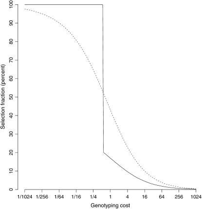
The optimal selection fraction is the value of α that maximizes this ratio (Figure 7). We observe a “phase transition” in the optimal selection fraction when the genotyping cost is approximately half that of raising and phenotyping an individual. If genotyping is very expensive, then we should genotype a small fraction of the population. As genotyping costs get smaller, the best strategy is to progressively genotype more individuals. If genotyping is cheaper than half the cost of phenotyping and rearing, the best strategy is to genotype everyone.

Figure 7.—

Optimal selection fraction as a function of genotyping cost for exponentially distributed waiting-time phenotypes. We assume a one-tail selective genotyping scheme is being used. The cost of genotyping is measured relative to the cost of raising and phenotyping, assuming everyone is followed up with no censoring. The dotted line gives the optimal selection fraction for two-tail selective genotyping when the trait is normally distributed. As expected, it is more efficient to genotype less as the cost of genotyping increases relative to raising and phenotyping. However, for one-tail selective genotyping there is a “phase transition” or a sudden change in the optimal fraction when the cost of genotyping is comparable to the cost of phenotyping and raising (by contrast, the change is gradual with traditional two-tail selective genotyping). The best strategy is to genotype everyone or <20% of the individuals depending on genotyping cost.

How should we choose the duration of follow-up?

For many lifetimes (time-to-event phenotypes), such as time to tumorigenesis (in animals), flowering time (in plants), and lifespan, an investigator may have to decide how long to wait for the event of interest (tumorigenesis, flowering, or death, in the examples above) to occur. Individuals for whom the event has not occurred in the follow-up period are considered “censored” in the language of survival analysis. For these individuals we do not know the time to event exactly, but we know that it is greater than the follow-up time.

We consider the problem of choosing the follow-up duration when measuring lifetimes. We consider the trade-offs between loss of information due to incomplete follow-up and the greater cost of full follow-up. We develop our ideas in the context of a backcross population.

Let y denote the time to an event and g denote the (0/1) genotype of an individual in a backcross when the event time distribution conditional on the genotype is exponential. Assume that the follow-up period for all individuals is T, 0 < T < ∞. Then, we can write

where f(·) is the density function of the event times, and is the survival function (the complement of the cumulative distribution function). Without loss of generality we rescale time so that the average waiting time for the “0” genotype is exp(−δ) and that of the “1” genotype is exp(δ). Then we obtain

We use this to construct the log-likelihood function and to derive the expected Fisher information for δ,

(4)

If C_f is the fixed cost per individual (for rearing and genotyping, for example), and C_w is the cost of waiting per unit time, then for follow-up period T the information–cost ratio is

where C = C_w/C_f. Thus, if we are willing to assume that the genetic effect, δ is small, we only need to maximize the ratio (1 − exp(−T))/(1 + TC). Elementary calculus shows that maximizing that ratio is equivalent to solving, for T, the equation

The solution of the equation, T*, the optimal time, has a one-to-one relationship with the optimal proportion of uncensored individuals, 1 − exp(−T*). Supplemental Figure 2 shows the optimal proportion of uncensored individuals as a function of C, the ratio of the cost of follow-up and the fixed costs per individual. As expected, the optimal follow-up fraction decreases with increasing follow-up cost. If the cost of following until the mean event time is approximately the same as the fixed costs for that individual, we should follow up until ∼70% of the events have been observed. The function, opt.wait in the R/qtlDesign package (Sen et al. 2007) calculates the optimal waiting time and the optimal proportion of uncensored individuals given the cost ratio, C.

How should we combine selective genotyping with choice of follow-up duration?

Selectively genotyping the longest-lived individuals is a good strategy for lifetime phenotypes. On the other hand, the longest lived are the most expensive to follow up and may be censored to save cost. What is the best strategy when a fraction of the longest-lived individuals are censored by design? We investigate this question when the lifetimes are exponentially distributed.

Suppose the individuals are followed up until time T. Treating T as a parameter, we can calculate the information gain function, and the expected information, as with the previously considered distributions. The expected information for small δ is

where β = exp(−T) is the proportion of censored individuals and ∧ is the maximum operator (Figure 6). Note that the upper bound for information with the β-proportion censored is β.

The information gain function for the censored exponential distribution is

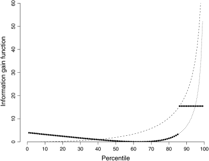
Figure 8 shows this function when the proportion censored is 15%. We can see that a one-tail selective genotyping strategy would be a good one, even in the presence of censoring.

Figure 8.—

Information gain function for exponential phenotypes in the presence of censoring. The dotted line shows the information gain function for uncensored individuals as a function of the percentile of their phenotype. The dashed line shows the level of the information gain function for censored individuals as a function of the percentile of individuals who are followed up. As an example, the solid dots show the information gain function for the case when all individuals above the 85th percentile are censored. The information gain function for the first 85% of individuals follows the usual pattern for exponential phenotypes. The information gain for the censored 15% of individuals is horizontal level, indicated by the dashed line. We see that one-tail selective genotyping is a good strategy even in the presence of censoring.

As with the case with no censoring, we investigated the effect of follow-up cost and genotyping cost on the genotyping/follow-up strategy. Let c_F be the cost of following up an individual for an average lifetime, and let c_G be the cost of genotyping an individual. Both costs are measured relative to the fixed cost of rearing an individual. Then the cost per individual of a study that genotypes α-proportion and censors β-proportion of the population is

and the information–cost ratio is

Given the cost structure, (c_F, c_G), we can find (α, β) that minimize the information–cost ratio (supplemental Figure 3).

The optimal selection fraction, α, shows an abrupt change, while the censoring proportion, β, increases gradually with follow-up cost. This is consistent with the optimal α when there is no censoring (β = 0) and the optimal β when everyone is genotyped (α = 1). The optimal censoring proportion is fairly insensitive to genotyping cost once genotyping cost is cheaper than the cost of rearing an individual. The optimal selection fraction is fairly insensitive to follow-up cost if follow-up cost is less than one-quarter of the cost of rearing.

DISCUSSION

In this article we have analyzed strategies in QTL experimental design in the context of nonnormal phenotype distributions and multilocus models. We analyze QTL study design by calculating the information content of design choices. Genotyping and phenotyping strategies can be analyzed using this framework. This approach can provide useful guidance for a range of scenarios more general than those considered in the literature so far.

Our central conclusions are the following:

1. Selective genotyping is effective for detecting linked and epistatic QTL as long as no locus has a large effect. When one or more loci have large effects, the effectiveness of selective genotyping is unpredictable—it may be heightened or diminished relative to the small-effects case. As a rule of thumb, if a locus explains ≥10% of the trait variation, then the effectiveness of selective genotyping for detecting other loci may be compromised.

2. Selective phenotyping efficiency decreases as the number of unlinked loci used for selection increases, and approaches random selection in the limit. However, when phenotyping is expensive, and a small fraction can be phenotyped, the efficiency of selective phenotyping is high compared to random sampling, even when >10 loci are used for selection.

3. For time-to-event phenotypes such as lifetimes, which have a long right tail, right-tail selective genotyping is more effective than two-tail selective genotyping. For heavy-tailed phenotype distributions, such as the Cauchy distribution, the most extreme phenotypic individuals are not the most informative.

4. When the phenotype distribution is exponential, and a right-tail selective genotyping strategy is used, the optimal selection fraction (proportion genotyped) is <20% or 100% depending on genotyping cost.

5. For time-to-event phenotypes where follow-up cost increases with the lifetime of the individual, one can calculate the optimal follow-up time that maximizes the information content of the experiment relative to its cost. For example, when the cost of following up an individual for the average lifetime in the population is approximately equal to the fixed costs of genotyping and breeding, the optimal strategy is to follow up ∼70% of the population.

A limitation of our approach is that it is model based, is asymptotic, and makes assumptions about the nature of the phenotype and genotype distributions. Our information analysis does not necessarily reflect how the data will be analyzed; a sample may be more informative, but the analysis method may not take full advantage of it. However, making design choices necessitates making assumptions about yet unseen data and making choices considering different scenarios. Our approach is flexible enough to permit explicit consideration of complexities that have not been contemplated for complex trait genetic study design.

Our information approach requires that we know (or guess) the conditional distribution of the phenotype given the genotype. In practice, only the marginal distribution of the phenotype is known, thus posing difficulties for our analytic approach. However, for the most interesting and useful scenarios, when the effect size is small, the marginal and conditional distributions are approximately the same. Thus, for the purposes of selecting a genotyping scheme, it is reasonable to use the marginal phenotype distribution as a guide.

Our analysis of selective genotyping was performed in the context of a backcross population where two genotypes segregate with equal frequency at each locus. Our current article does not conclusively establish how generally applicable the results are to F₂ intercrosses and human association studies with multiple haplotypes. However, there are reasons to expect that the conclusions apply more generally. Sen et al. (2005) showed that expected information under selective genotyping for any contrast between haplotypes in an association study behaves the same way as in a backcross. Our simulation study provides further support for the idea that selective genotyping is effective in the context of multiple QTL as long as the individual effects of each locus are small. Further work would be needed to provide explicit quantitative guidelines regarding when we may expect the payoff from selective genotyping to break down in nonbackcross populations.

How small should the effect of individual loci be for selective genotyping to be effective? The answer depends on the underlying genetic mode of action, which is not known in advance, and also on the experiment's cost structure. Examining Figures 1 and 2 suggests that if no locus contributes >20% of the phenotypic variance in a backcross population, the expected information gain from selective genotyping is close to what would be predicted if a single locus contributed to the trait. We expect individual loci to explain much smaller fractions of the variance for complex traits. This leads us to conclude that selective genotyping would be effective in reducing the genotyping cost for complex traits with a single phenotype of interest.

Our results show how follow-up time for time-to-event phenotypes can be optimized in conjunction with selective genotyping. If subject recruitment and follow-up is a dominant contributor to study cost, these results may have a significant impact. We note, however, that experimenters should carefully choose the cost function to reflect the cost structure of their study. We used a linear cost function in our analysis, for convenience, but that may frequently not be the correct choice. In such cases, the cost–information trade-offs should be recalculated to obtain choices better suited to the study at hand. More generally, there is the broader question: How should we value a study, and how would that impact study design (Bacchetti et al. 2008)? Our approach implicitly valued a study by its information–cost ratio; other ways of valuing a study would lead to different results.

The optimal selection fraction for one-tail selective genotyping with exponentially distributed phenotypes exhibits a discontinuity. This is surprising, and probably undesirable. However, as we have noted, it is not the most efficient genotyping strategy, but a “good” one that is easily implemented. A strategy devised using the information gain function will have expected information equaling or exceeding that for one-tail selective genotyping. That strategy will not exhibit a discontinuity in the optimal genotyping fraction as a function of cost.

Our analysis of selective genotyping for nonnormal trait distributions has led us to conclusions similar to those of Park (1996) and Zheng and Gastwirth (2000) who used more involved analytical techniques calculating the exact distribution of order statistics. They asked the question “Where does the Fisher information in order statistics lie?” For prioritizing individuals for genotyping we ask the related question: “Where does the Fisher information in the quantiles lie?” For this question we were able to use asymptotic results that are obtained more easily than the exact results for order statistics. A biproduct of our approach is the information gain function that can be used to devise selective genotyping strategies appropriate for any trait distribution.

The next wave of genetic studies is expected to collect high-dimensional data using various “omic” technologies. In these studies, somewhat different study design questions from those considered in this article might arise. For example, for two-color microarrays, a selective phenotyping approach has to consider pairing of samples per array. Fu and Jansen (2006) proposed using a distant-pair design, using an information approach for this setting. Another question might be “How should one select individuals for microarray phenotyping based on a trait of interest and genotypes at a locus of interest?” The information approach may be used in this setting as well, but this requires further development.

Finally, although power calculations have a justified place in guiding study design, they depend on the unknown effect size and change nonlinearly with sample size. This has led some to question their dominant role in determining study design in biomedical research (Bacchetti et al. 2008). Information is arguably a better criterion, although it too has to be used judiciously in conjunction with the cost structure of the study and perhaps the value (which is harder to quantify). Relative to calculating power, calculating information is harder and sometimes impossible; our work shows that for some genetic studies information can be calculated explicitly using algebraic or numeric approximations. This may help us make more realistic study design choices than those based on power calculations alone.

Computer code used for symbolic algebra using Maxima (http://maxima.sourceforge.net) and for numerical calculation (including code for generating figures) using R (http://www.r-project.org) is available at http://www.epibiostat.ucsf.edu/biostat/sen.

References

- Abasht, B., and S. J. Lamont, 2007. Genome-wide association analysis reveals cryptic alleles as an important factor in heterosis for fatness in chicken F2 population. Anim. Genet. 38 491–498. [DOI] [PubMed] [Google Scholar]
- Bacchetti, P., C. McCulloch and M. Segal, 2008. Simple, defensible sample sizes based on cost efficiency. Biometrics 64 577–585. [DOI] [PMC free article] [PubMed] [Google Scholar]
- Carr, L., K. Habegger, J. Spence, L. Liu, L. Lumeng et al., 2006. Development of congenic rat strains for alcohol consumption derived from the alcohol-preferring and nonpreferring rats. Behav. Genet. 36 285–290. [DOI] [PubMed] [Google Scholar]
- Chen, Z., G. Zheng, K. Ghosh and Z. Li, 2005. Linkage disequilibrium mapping of quantitative-trait loci by selective genotyping. Am. J. Hum. Genet. 77 661–669. [DOI] [PMC free article] [PubMed] [Google Scholar]
- Cox, D., and N. Reid, 2000. The Theory of the Design of Experiments. Chapman & Hall/CRC, London/New York/Cleveland, OH/Boca Raton, FL.
- Darvasi, A., and M. Soller, 1992. Selective genotyping for determination of linkage between a marker locus and a quantitative trait locus. Theor. Appl. Genet. 85 353–359. [DOI] [PubMed] [Google Scholar]
- Frankel, W., and N. Schork, 1996. Who's afraid of epistasis? Nat. Genet. 14 371–373. [DOI] [PubMed] [Google Scholar]
- Fu, J., and R. Jansen, 2006. Optimal design and analysis of genetic studies on gene expression. Genetics 172 1993–1999. [DOI] [PMC free article] [PubMed] [Google Scholar]
- Gallais, A., L. Moreau and A. Charcosset, 2007. Detection of marker-QTL associations by studying change in marker frequencies with selection. Theor. Appl. Genet. 114 669–681. [DOI] [PubMed] [Google Scholar]
- Huang, B., and D. Lin, 2007. Efficient association mapping of quantitative trait loci with selective genotyping. Am. J. Hum. Genet. 80 567–576. [DOI] [PMC free article] [PubMed] [Google Scholar]
- Jansen, R. C., and J. P. Nap, 2001. Genetical genomics: the added value from segregation. Trends Genet. 17 388–391. [DOI] [PubMed] [Google Scholar]
- Jin, C., H. Lan, A. D. Attie, G. A. Churchill and B. S. Yandell, 2004. Selective phenotyping for increased efficiency in genetic mapping studies. Genetics 168 2285–2293. [DOI] [PMC free article] [PubMed] [Google Scholar]
- Lander, E. S., and D. Botstein, 1989. Mapping Mendelian factors underlying quantitative traits using RFLP linkage maps. Genetics 121 185–199. [DOI] [PMC free article] [PubMed] [Google Scholar]
- Lebowitz, R., M. Soller and J. Beckmann, 1987. Trait-based analyses for the detection of linkage between marker loci and quantitative trait loci in crosses between inbred lines. Theor. Appl. Genet. 73 556–562. [DOI] [PubMed] [Google Scholar]
- Lynch, M., and B. Walsh, 1998. Genetics and Analysis of Quantitative Traits. Sinauer Associates, Sunderland, MA.
- McLachlan, G. J., and T. Krishnan, 1996. The EM Algorithm and Extensions. John Wiley & Sons, New York.
- Ohno, Y., H. Tanase, T. Nabika, K. Otsuka, T. Sasaki et al., 2000. Selective genotyping with epistasis can be utilized for a major quantitative trait locus mapping in hypertension in rats. Genetics 155 785–792. [DOI] [PMC free article] [PubMed] [Google Scholar]
- Orchard, T., and M. Woodbury, 1972. A missing information principle: theory and applications. Proceedings of the 6th Berkeley Symposium on Mathematical Statistics, Berkeley, CA, Vol. 1, pp. 697–715.
- Park, S., 1996. Fisher information in order statistics. J. Am. Stat. Assoc. 91 385–390. [Google Scholar]
- Rapp, J. P., 2000. Genetic analysis of inherited hypertension in the rat. Physiol. Rev. 80 131–172. [DOI] [PubMed] [Google Scholar]
- Sen, S., J. M. Satagopan and G. A. Churchill, 2005. Quantitative trait loci study design from an information perspective. Genetics 170 447–464. [DOI] [PMC free article] [PubMed] [Google Scholar]
- Sen, S., J. M. Satagopan, K. W. Broman and G. A. Churchill, 2007. R/qtlDesign: inbred line cross experimental design. Mamm. Genome 18 87–93. [DOI] [PMC free article] [PubMed] [Google Scholar]
- Wallace, C., J. Chapman and D. Clayton, 2006. Improved power offered by a score test for linkage disequilibrium mapping of quantitative-trait loci by selective genotyping. Am. J. Hum. Genet. 78 498–504. [DOI] [PMC free article] [PubMed] [Google Scholar]
- Zheng, G., and J. L. Gastwirth, 2000. Where is the Fisher information in an ordered sample? Stat. Sin. 10 1267–1280. [Google Scholar]