Stimulus Dependency and Mechanisms of Surround Modulation in Cortical Area MT

Abstract

The perceptual interpretation of a given visual feature depends on the surrounding context. To explore the neural mechanisms underlying such contextual interactions in the motion domain, we studied responses of neurons in the middle temporal area (MT) of macaque monkeys while presenting a variety of center-surround stimuli that stimulated both the classical receptive visual field (CRF) and the receptive field surround. In human psychophysical experiments, the perceptual impact of the surround stimulus on the center stimulus varied from motion capture (“integration”) to motion contrast (“segmentation”). In our neurophysiological experiments, the directional tuning of surround modulation with these stimuli ranged from antagonistic (consistent with motion contrast) to integrative (consistent with motion capture) and agreed qualitatively with perception under some but not all conditions. Most strikingly, for a stimulus that elicited perceptual motion contrast, surround modulation was integrative if the CRF stimulus was ambiguous due to the aperture problem. In addition, we found that surround modulation was linked to response magnitude: stimuli eliciting the largest responses yielded the strongest antagonism and those eliciting the smallest responses yielded the strongest integration. We developed a neural network model that accounts for this finding as well as a previous finding that surround suppression in area MT is contrast-dependent. Our findings suggest that changes in MT surround modulation result from shifts in the balance between directionally tuned excitation and inhibition mediated by changes in input strength. We speculate that input strength is, in turn, linked with the ambiguity of the motion present within the CRF.

Introduction

The ability of stimuli outside the classical receptive field (CRF) of sensory neurons to modulate responses to stimuli within the CRF is well established. In contrast, the function of such surround modulation is less clear (Allman et al., 1985b; Gilbert, 1992; Fitzpatrick, 2000; Tadin et al., 2003) (for review, see Albright and Stoner, 2002). For the middle temporal area (MT), which is specialized for visual motion processing, numerous studies have reported that the tuning of surround modulation is typically antagonistic with respect to the CRF: stimuli moving in a direction that is preferred within the CRF lead to smaller responses when added to the surround than do stimuli that are less preferred (Allman et al., 1985a; Tanaka et al., 1986; Xiao et al., 1997; Bradley and Andersen, 1998). It has been proposed that this surround antagonism functions to segment the visual image into distinct objects (Allman et al., 1985b; Bradley and Andersen, 1998).

Visual motion perception relies on integration as well as segmentation (Braddick, 1993). Whereas segmentation parses the image into independently moving objects, integration pools information from adjacent locations to create a representation of coherent motion. To support perceptual integration, the addition of a surround stimulus to a CRF stimulus should elicit integrative modulation: responses should be larger when the surround stimulus moves in a direction that is “preferred” (i.e., for stimuli within the CRF) than when it moves in a less preferred direction. Consistent with the importance of these opposing operations in perception, we have recently discovered that surround modulation within area MT can be either antagonistic or integrative depending upon the stimulus (Huang et al., 2007). This finding demonstrated that surround modulation in area MT is stimulus-dependent, but posed several fundamental questions regarding both function and mechanism.

In this study, we sought to address the questions posed by our first study. In our previous study, the stimuli that yielded surround integration were moving squares with one contour centered within the CRF. Replacing the contour within the CRF with random dots yielded mostly surround antagonism. These “contour” and “dot” stimuli differed in both the physical attributes of the stimulus present in the CRF and in perceptual interpretation. In this study, we introduced stimuli that allowed the contribution of these two differences to be teased apart. We found that neuronal responses paralleled perception (as assayed in human subjects) for dot and contour stimuli but not for our new stimuli. Most strikingly, stimuli that offered ambiguous motion in the CRF (i.e., the “aperture problem”) yielded integrative modulation although they elicited perceptual segmentation. This finding suggests that the directional tuning of surround modulation is determined by the ambiguity within each MT neuron's CRF partly independent of perceptual interpretation. Consistent with previous findings, we also found that response magnitude was generally greater for stimuli that provided unambiguous motion information within the CRF than for stimuli that provided ambiguous motion information. Moreover, we found a systematic relationship between response strength and surround modulation: stimuli that drove neurons relatively weakly yielded integration, stimuli that drove neurons strongly elicited antagonism, and intermediate stimuli elicited intermediate interactions. We devised a neural network model that accounts for this relationship as well as previous reports of contrast-dependent surround suppression within area MT.

Materials and Methods

General

We conducted psychophysical experiments using human subjects and neurophysiological experiments on rhesus monkeys. Visual stimuli were identical for both sets of experiments except where noted.

Psychophysical experiments

Subjects

Three naive human subjects (G.B., M.N., and M.T.) and one of the authors (X.H.) were subjects in the psychophysical experiments. Participants gave informed consent, and all procedures were in accordance with international standards (Declaration of Helsinki) and National Institutes of Health guidelines. All subjects had normal or corrected-to-normal visual acuity. Each subject's head was stabilized with a chin rest.

Visual stimuli

Visual stimuli were presented on a 19″ CRT monitor (1024 × 768 pixel resolution and 75 Hz refresh rate) at a viewing distance of 57 cm. The visual stimuli were the same (in spatial configuration, dimensions, luminance, motion direction and speed, etc.) as those used in the neurophysiological experiments, with a few additional manipulations to allow the perceptual report of motion directions (described in Behavioral Paradigm). Visual stimuli included contour, corner, dot, and bar stimuli (described in Neurophysiological experiments). As was true during most of our neuronal recordings (except for the minority of neurons with eccentric CRFs), stimuli were positioned so that the fixation target was inside the stimulus boundaries. Figure 1A illustrates the stimulus set.

Figure 1.

Visual stimuli and behavioral paradigm. A, Center-surround stimuli. Top (left to right), Contour, corner, and control stimuli. Bottom (left to right), Dot, long-bar, and short-bar stimuli. Annuli correspond to either the CRF (neurophysiology) or the cue indicating the feature whose motion was to be reported (psychophysics). Stationary stimuli were initially presented at center of the monitor. The positioning of features within the CRF or cue was achieved by varying the position of the fixation target. Note that, except for corner stimuli, all stimuli differed only in the feature that moved within the CRF or cued region. B, Behavioral paradigm. Fixation target appeared first. After fixation was achieved, each stimulus was stationary for 500 ms and then moved for 500 ms. Upon completion of a trial, human subjects reported the direction of perceived motion. Monkeys were not required to make a report but, instead, were given a juice reward if fixation had been adequately maintained.

Behavioral paradigm

The human behavioral paradigm closely matched that of our neurophysiological experiments (Fig. 1B). At the beginning of each trial, the static visual stimulus and the fixation target (a square 0.2 by 0.2 degrees) appeared on the video monitor. Subjects indicated by keypress when they had obtained fixation and two hundred milliseconds later, one portion of that stimulus was cued by the appearance of a red annulus (7° diameter, 0.1° thick, 200 ms duration). The location of this cue corresponds to that of the CRF in our neurophysiological experiments. Accordingly, the cue was centered over either one of the corners (corner stimuli) or one of the sides of the square (contour, dot, short-bar, and long-bar stimuli). If the latter, then the cue was centered over the appropriate feature: a contour (contour stimuli), dots (dot stimuli) or a bar (short- and long-bar stimuli). Any of the four sides or the four corners could be cued, but to match the conditions of our neurophysiology experiments (in which stimuli were positioned relative to the CRF), the cued location (i.e., relative to fixation) in each block of 20 trials was fixed. The corner or side of the square that was cued was varied across blocks of trials. The fixation spot was always positioned within the interior of the square and displaced 3.54° horizontally and vertically from the center of the cued feature. This resulted in the cued feature being 5° from fixation. This eccentricity was chosen to be representative of receptive field centers of our neuronal sample. For each of the 4 cued sides, there were 2 fixation placements yielding a total of 8 blocks.

In the context of our psychophysical experiments, the “local” motion direction refers to the motion of the stimulus feature centered within the cue and the “global” motion direction refers to the motion of the stimulus outside the cue. After cue offset, stimuli remained static for 100 ms and then moved in one of the four global directions (45, 135, 225 and 315°) for 500 ms, after which they disappeared. Subjects were required to maintain fixation throughout the trial until 500 ms after the stimulus offset, at which time the fixation spot was extinguished. Following fixation offset, polar coordinates (a 10° diameter circle with angular markings) were displayed. Subjects adjusted the angle of an oriented bar (5° long, one end was anchored at the coordinate origin) from 0 to 360° to indicate the perceived direction of the cued feature. The angular adjustment step was 1°. Subjects pressed a key to register their response. If a subject was not satisfied with their report for any reason, they could press a different key and repeat the trial. Each subject completed 160 trials (i.e., 20 trials per block times 8 blocks). Trials in which subjects waited too long to input a response were not registered so the actual number of valid trials was slightly less (1–4% less depending upon the subject).

Data analysis

For each subject, trials in different blocks were pooled together after transforming directional reports into a common coordinate frame. Accordingly, the local motion direction was, except for corner stimuli, defined as 0° and the global motion direction was defined as 45°. For corner stimuli, the motion within the cued region was the same as the global motion (i.e., 45°). The mean and the variance of perceptual reports were calculated for each stimulus type. Data from all subjects were pooled together and population probability distributions were computed.

Neurophysiological experiments

Subjects

Three adult male rhesus monkeys (Macaca mulatta; monkeys F, C, and B) were used in the neurophysiological experiments. Experimental protocols were approved by the Salk Institute Animal Care and Use Committee and conform to U. S. Department of Agriculture regulations and to the National Institutes of Health guidelines for the care and use of laboratory animals. Procedure for surgical preparation, behavioral training, and electrophysiological recording were routine and similar to those described previously (Duncan et al., 2000; Krekelberg and Albright, 2005). Briefly, each monkey was implanted with a stainless steel head post and a recording cylinder oriented vertically allowing recording from neurons in area MT. The positioning of the chamber was guided by magnetic resonance imaging scans obtained at the University of California, San Diego, Center for Magnetic Resonance Imaging. During neural recording, monkeys were seated in a standard primate chair (Crist Instruments) with the head post rigidly supported by the chair frame to prevent head movement.

Visual stimuli

Stimulus presentation, behavioral paradigm, and data acquisition were controlled by specialized “CORTEX” software (Laboratory of Neuropsychology, National Institute of Mental Health, Bethesda, MD; http://www.cortex.salk.edu). Visual stimuli were presented on a 21″ CRT monitor at a viewing distance of 57 cm. Monitor resolution was 1024 × 768 pixels and the refresh rate was 75 Hz. The output of the video monitor was measured with a PR650 photometer (Photo-Research). All visual stimuli were presented while monkeys performed a visual fixation task (see Behavioral paradigm). Stimuli are described in the relevant sections below.

Initial estimate of preferred direction.

Before CRF mapping, we estimated preferred direction using a large random-dot patch (30° × 30°) undergoing circular translation (Schoppmann and Hoffmann, 1976). Dot luminance was 13.6 cd/m² and background luminance was 0.67 cd/m². This method allows a continuous and complete mapping of directional responses in a single trial. Ten to twenty trials were typically used to estimate the preferred direction of each neuron. This method has been shown to agree nicely with conventional methods for estimating preferred direction (see below).

CRF mapping.

CRFs were mapped by recording responses to square-wave gratings which drifted in the preferred direction as estimated above. Gratings were presented within individual squares of a spatial grid (usually 25° × 20°, sometimes 40° × 30°) with grid lines separated by 5°. Each square (and hence each grating) in this grid was 5° × 5°. Gratings appeared, were static for 50 ms and then moved for 500 ms. Only one grating was shown per trial. The raw CRF map was interpolated using the Matlab (MathWorks) function “interp2” at an interval of 0.5°, using “bicubic” interpolation. The location in the interpolated map giving rise to the highest firing rate was taken as the CRF center over which stimuli were then centered. Gratings were presented one at a time at least 5 times at each spatial location until the CRF map stabilized.

Characterization of directional tuning.

Once we mapped the CRF, we characterized directional tuning using square-wave gratings drifting in one of eight directions at 10°/s. The gratings were viewed through an invisible circular aperture with a diameter of 6° centered on the CRF. Preferred direction was determined using an on-line analysis script running in Matlab. With few exceptions, and consistent with previous findings, the preferred direction estimated this way matched the initial estimation of the preferred direction using the circular translation stimuli described above. For those exceptions, CRF mapping was repeated using the newly determined preferred direction.

Center-surround stimuli.

The stimuli used to characterize surround modulation were variations of outlined squares. The local motion direction refers to the motion of the feature centered within the CRF. Within the CRF, motion was restricted to two local directions along a single axis (see Contour and corner stimuli). The global motion direction refers to the motion of the stimulus outside the CRF (i.e., the “surround stimulus”). Stimuli moved in one of four global directions at 5°/s: 45, 135, 225 and 315°, with 0° defined as rightward and angles incremented counterclockwise. The outlined portion of the square had a luminance of 13.6 cd/m². The interior of the square and the background were identical with a luminance of 0.67 cd/m². Squares were 20° across and contour width (i.e., of the outline) was 0.5°. Stimuli were presented at the center of the video monitor. The appropriate portion of the square (i.e., either a side or a corner of the square, see below) was positioned within the CRF by varying the position of the fixation target. The fixation target was positioned to minimize the eccentricity of the stimulus as a whole. In consequence, for CRFs with eccentricities <10 degrees, the fixation target was positioned within the center-surround stimulus initially (i.e., before the motion of the stimulus). Figure 1A illustrates the center-surround stimulus set and positioning of fixation target.

Contour and corner stimuli.

Contour and “corner” stimuli were both outlined squares, differing only in how they were positioned relative to the CRF. For contour stimuli, either a horizontal or vertical contour (i.e., a side) of the square was centered within the CRF. As a consequence, the two local motions within the CRF (i.e., the directional component orthogonal to the orientation of the contour within the CRF) were either vertical (i.e., up or downward) or horizontal (i.e., left or rightward). The four global motions of the square (see above) were, conversely, the same for all neurons. The choice of either placing a horizontal or a vertical contour inside the CRF was based on the directional selectivity of the neuron under study to maximize the difference between the responses to the global and local motions. The beginning position of the contour was the same for all four directions of global motion. For corner stimuli, one corner of the square was centered on the CRF and the square moved in one of the four global directions (again the beginning position was the same for all four directions). The motion of the corner was unambiguous and consequently, for corner stimuli, the motion within the CRF was identical to the global motion of the square.

Dot stimuli.

Dot stimuli were created by replacing the “CRF contour” (i.e., the contour passing through the CRF) of the contour stimulus with random dots viewed through an invisible circular aperture. This aperture was static and had a diameter of 4°, which matched the length of the contour's path (including the width of the contour) for both directions of motion. The dots were of the same luminance as the contour and had the same velocity as the local motion of that contour. Based on a SD metric for nonperiodic stimuli (Moulden et al., 1990), the luminance contrast of dot stimuli was 14.7 cd/m². Dot density was ∼3 dots per square degree. The diameter of each dot was ∼0.2°.

Long- and short-bar stimuli.

“Bar” stimuli were created by introducing gaps between the CRF contour and the rest of the square. For “short-bar” stimuli, these gaps were 7.5° in length resulting in a moving segment (i.e., a bar) within the CRF that was 4° in length. For “long-bar” stimuli these gaps were 3.75° in length resulting in a moving segment within the CRF that was 11.5° in length. The gap and bar lengths add up to 19 ° whereas each side is 20°. The “missing” degree comes from the widths (0.5°) of the orthogonal contours. This manipulation disrupted figural continuity and resulted in a perception of motion contrast. The bars within the CRF were of the same widths as the contour they replaced and moved in the same local motions (i.e., measured orthogonal to its orientation) as that contour. The stimulus motions in the surround were identical for bar and contour stimuli.

Control stimuli.

“Control” stimuli were identical to contour stimuli except that the CRF contour was erased. Since all segments (even those abutting the other contours) of the CRF contour provide the same ambiguous motion information, our control stimulus necessarily corresponds to the portion of our experimental stimuli responsible for directional surround modulation. Our control stimulus was identical to the surround portion (i.e., the portion of the stimulus other than that centered in the CRF) of dot and bar stimuli.

Bar-control stimuli.

“Bar-control” stimuli were squares with the bars (i.e., short- or long-bars) deleted. Bar-control stimuli thus precisely complemented the individual bars of the short- and long-bar stimuli and moved with the same speed and in the same two directions (i.e., local not global directions) as the bars and CRF contours (see Fig. 8A, bottom). In addition, we also recorded responses from a subset of neurons to intact squares (i.e., without the bars deleted) that moved in the local directions and with the same local speed as the bars and CRF contours (see Contextual modulation index).

Figure 8.

Role of CRF ambiguity in surround integration. A, Long-bar stimulus (top) and long-bar control stimulus (bottom). The long-bar control stimulus corresponded to the complement of the bar within the CRF and moved in the same two local directions (indicated by arrows). Neurons that did not respond to this stimulus were judged to be subject to the aperture problem for long-bar stimuli. Short-bar control stimuli were constructed similarly (see Materials and Methods). B, Role of aperture problem in surround integration. For neurons subject to the aperture problem for long-bar stimuli, the average CMI was 0.24. This value was significantly positive (indicated by asterisk) and significantly different from the average CMI of 0.037 for neurons that were not subject to the aperture problem for those stimuli (t test p < 0.05). In response to contour stimuli, the average CMIs for these two groups of neurons (light gray bars) were both significantly positive (indicated by asterisks) and were not significantly different from each other. Error bars indicate SE.

Stimulus blocks

We conducted two sets of experiments. In the first set, we recorded neuronal responses to contour and dot stimuli. In the second set, we recorded neuronal responses to contour, corner, control, short- and long-bar stimuli. In both sets of experiments, stimuli were interleaved within a block of trials. We introduced the second stimulus set after we had already acquired data using the first, but some cells were tested with both sets (in separate blocks of trials). To compare response magnitudes across all stimulus types, we normalized responses relative to the contour stimulus within each of these interleaved stimulus sets and then pooled these normalized responses for each stimulus type. This approach avoids confounding stimulus-specific variation in firing rate with apparent changes in firing rate due to changes in neuronal isolation or actual changes in overall neuronal responsivity.

Behavioral paradigm

In one monkey subject (monkey F), a monocular scleral search coil was implanted to monitor eye positions. For the other two monkeys, eye positions were sampled at 60 Hz using an infrared video-based tracking system (Iscan). Monkeys were required to maintain fixation within a 2° × 2° window during the experiment trial. Actual fixation was typically much more accurate than this window size. The fixation target was positioned so that the appropriate stimulus feature (i.e., contour, dots, or bar) was centered within the receptive field. On each trial, after a monkey had acquired and maintained fixation for 200 ms, visual stimuli appeared and remained static for 500 ms. Visual stimuli then moved with a constant velocity for another 500 ms. Upon successful completion of a trial, monkeys were given a small juice reward. Figure 1B illustrates the trial sequence.

Electrophysiological recording

Magnetic resonance imaging (MRI) scans were used to guide electrode placement. We identified area MT by its characteristically large proportion of directionally selective cells, small CRFs relative to those of neighboring area MST, and its location on the posterior bank of the superior temporal sulcus. Recording depths of physiologically identified MT neurons agreed well with the expected anatomical location based on the structural MRI scans. Action potentials were classified as “single-unit” (i.e., as coming from an individual neuron) if those waveforms were, based on the raw waveforms and the PCA analysis of the Plexon spike sorter, clearly clustered and distinct from the baseline noise and other clusters of spikes. Action potentials that crossed a magnitude threshold and had stable waveforms but did not meet the criteria for a single-unit were grouped together and classified as “multiunit.”

Data analysis

Screening criteria.

As noted above, our control stimulus corresponded to the portion of our contour stimulus that distinguished the local motion of the contour within the CRF from the global motion of the square. Accordingly, if neurons responded to this control stimulus, we assumed that this key portion of the surround stimulus intruded into the CRF, else we assumed that it did not. We evaluated responses to control stimuli using two criteria, which enabled us to classify neurons into “no-control-response” and “control-response” samples. All neurons with a significant difference (Wilcoxon signed rank test, p < 0.05) in either of these two types of comparisons were classified as control-response neurons. The remaining neurons were classified as no-control-response neurons. First, neuronal activity in the period 0–500 ms after the motion onset of control stimuli could not be significantly greater than baseline activity (measured in the 200 ms before stimulus onset) of the corresponding condition (Wilcoxon signed rank test, p > 0.05). We imposed this criterion upon all four (global) directions of stimulus motion. Second, we compared “responses” to the control stimuli that corresponded to the contour stimuli with the same local motions within the CRF. There were two such comparisons. To illustrate, for the example in Figure 3C, the activity seen in the upper-left PSTH was compared with that seen in upper-right PSTH, and the activity seen in the lower-left PSTH was compared with that seen in the lower-right PSTH. These two comparisons correspond to upward and downward local motions within the CRF, respectively (see Fig. 3B). Because we wished to be conservative in our identification of no-control response neurons, Bonferroni correction for multiple comparisons was not imposed on these criteria. As a result, the criteria for detecting responses to control stimuli were much stricter than the criterion for each individual test.

Figure 3.

No-control-response neuron with integrative surround modulation. Responses to the four global motions of stimuli are shown as PSTHs and response vectors (black lines) in which angles indicate the direction of global motion (i.e., of the surround stimulus) and lengths indicate response magnitude for that direction. A, Responses to corner stimuli. The motion period (dark bar) was, for all stimuli, from 500 to 1000 ms after stimulus onset. For this neuron, the P direction was up and to the left. We define the global prediction (blue arrow) as the direction of the average of the four corner response vectors (see Results, Responses of MT neurons to contour stimuli: integrative modulation). B, Responses to contour stimuli. Local motion refers to the motion of the contour within the CRF. For this example, the local motion was either upward or downward. The P direction of global motion resulted in upward local motion. For this example, the PP direction is thus up and to the right. Responses to the P direction were larger than to the PP direction indicating integrative surround modulation. The contour preferred direction (red arrow) is the direction of the average of the four contour response vectors. C, We classified this neuron as a no-control-response neuron because control stimuli did not elicit significant responses. D, Directional tuning measured with drifting gratings. Responses to gratings moving in the two local motion directions determine the local prediction. For this neuron the two local directions were upward and downward. Since responses to upward motion were greater than to downward motion, the local prediction (green arrow) points upward. E, The contour preferred direction (red arrow) is superimposed on the local (green arrow) and global (blue arrow) predictions. The contour preferred direction is biased away from the local prediction toward the global prediction indicating integrative surround modulation.

Testing for nonlinear directional interactions.

We used a boot-strapping method to determine whether neuronal responses to contour stimuli revealed nonlinear center-surround interactions. In particular, we compared responses to the preferred (P) and preferred-pair (PP) global directions. The P direction is defined as the global direction that evokes the largest response to corner stimuli. The PP direction is defined as the global direction that shares the same local motion (i.e., the same motion within the CRF) as the P direction. Note that P refers only to the particular global direction (i.e., of the four global directions) that yielded the largest response, not to the overall preferred direction. To illustrate, if the P direction were up and to the right and a vertical contour of the contour stimulus was within the CRF, then the PP direction would be down and to the right: those two global directions yield the same local (i.e., rightward) motion within the CRF.

We sampled Contour responses to P and PP directions 5000 times with replacement. For each pair of sampled responses, we subtracted the response to the PP direction from that to the P direction. In this way, we obtained a distribution of the response differences between the contour responses to P and PP directions. Using the same methods, we also obtained a distribution of these response differences for control stimuli. We then tested if the two distributions were significantly different using a t test at a significance level of 0.05. Neurons for which those two distributions were significantly different were classified as “nonlinear” and the rest were classified as “linear.”

Contextual modulation index.

We created a bounded measure that characterizes the directional selectivity of surround modulation with respect to the CRF. Unlike our bootstrap analysis, which only addressed differences in responses to the P and PP directions (see above), this measure incorporates responses to all four global directions. This contextual modulation index (CMI) is 1 for modulation that is maximally integrative, −1 for modulation that is maximally antagonistic, and 0 for untuned modulation.

To compute this metric, we first estimated the preferred directions for each of the center-surround stimuli with which the neuron had been tested (i.e., contour, dot, short- and long-bar stimuli). We defined the “preferred direction” for each stimulus as the direction of the vector average of the four response vectors. The angle of these response vectors corresponds to the global motion of the stimulus and their length corresponds to the response magnitude elicited by that direction of motion. The preferred direction so-computed is the direction of motion that would be expected to give the largest response and is thus distinguished from the P global direction (see above). Where appropriate, we refer to each of these preferred directions by stimulus type: “contour preferred direction,” “dot preferred direction,” etc. We then compared these preferred directions with global and “local predictions.” The “global prediction” is the reference point for maximal surround integration and corresponds to the preferred direction obtained using stimuli moving through the CRF in each of the four global directions. If the preferred direction for a particular stimulus is close to the global prediction, this implies that a neuron is responding as if the surround portion of that stimulus were in the CRF. For the analyses presented here, the corner stimulus was used to derive the global prediction (see Figs. 3A, 4A). The global prediction can also be based on responses to gratings drifting in the global directions. The preferred directions for corner and grating stimuli were in strong agreement and, unsurprisingly, we found that using gratings to establish the global prediction yielded the same overall pattern of results as using corner stimuli.

Figure 4.

Control-response neuron with integrative surround modulation. Panel arrangements and conventions are same as in Figure 3. A, Responses to corner stimuli. The corner response was strongest when the global direction was up and to the right (the P global direction). The direction of the averaged corner response vectors is the global prediction (blue arrow). B, Responses to contour stimuli. For this neuron, the local motion was rightward for the P direction, and hence the PP global direction was down and to the right. The motion of the contour centered within the CRF was the same for P and PP directions. Responses to the P direction were larger than to the PP direction indicating integrative surround modulation. The direction of the averaged contour response vectors is the contour preferred direction (red arrow). C, We classified this neuron as a control-response neuron since control stimuli elicited weak but significant responses. D, Directional tuning measured with drifting gratings. The motion of the contour within the CRF (i.e., the local motion) was leftward or rightward and hence responses to those two directions were used to produce the local prediction (green arrow). Responses to rightward motion were stronger than to leftward motion and hence the local prediction points rightward. E, The contour preferred direction (red arrow) is superimposed on the local (green arrow) and global (blue arrow) predictions. The contour preferred direction is biased away from the local prediction toward the global prediction indicating integrative surround modulation.

The local prediction is the preferred direction for the single axis of motion defined by the two local motions within the CRF. This directional preference was determined by examining responses to gratings moving in those two directions (see Figs. 3D, 4D). To illustrate, for the neuron whose responses are illustrated in Figure 3, the relevant axis of motion is vertical as the CRF contour of the Contour stimulus moves either upward or downward (see Fig. 3B). The local prediction is upward as gratings moving in that direction elicited a larger response than did gratings moving downward. Alignment of the preferred direction for a particular stimulus with the local prediction implies that a neuron is only selective for motion within the CRF. For a subset of neurons (n = 117), we also constructed local predictions based on responses to squares moving in the local directions (see bar-control stimuli, above). The local predictions based on responses to gratings and squares nearly always agreed.

The CMI was defined as follows:

ϕ is the angular difference between the preferred direction for a particular stimulus and the local prediction (see Fig. 5A). θ is the angular difference between the global prediction and the local prediction. θ could in principle be as large as 180°, but most neurons (76%) yielded θs <90°. Such neurons usually had unimodal tuning curves that were fairly symmetrical about the preferred direction. A minority of neurons, however, had θs >90° (24%) or even >120° (5%). These neurons had tuning curves that were asymmetric around the preferred direction and/or had multiple peaks. The data from neurons with θs >90° were not qualitatively different from that from neurons with smaller θs.

Figure 5.

A, CMI definition. The CMI is based on the ratio of ϕ and θ. ϕ is the angular difference between the directional preference for a particular stimulus (e.g., the contour preferred direction) and the local prediction. θ is the angular difference between the global and local predictions. The CMI varies from −1 to 1 as ϕ varies from −θ to θ and its magnitude falls off linearly as the absolute value of ϕ deviates from θ. B, Scatter plot of ϕ versus θ. In this illustration, θ is defined to be positive (i.e., the absolute value of the difference between the global and local predictions). Positive and negative ϕs indicate integrative and antagonistic modulation. The top and bottom diagonal lines indicate CMIs of 1 and −1, respectively. As indicated in Figure 5A, the magnitude of the CMI falls off as the distance from these two diagonals increases so that, for example, points above the top diagonal have CMIs <1. C, CMI frequency distribution. The CMIs for the two example neurons shown in Figures 3 and 4 are 0.80 and 0.63, respectively: both neurons exhibited motion integration. Of the 279 neurons in our sample, the observed surround modulation of 250 was readily interpretable as either integrative or antagonistic. The mean CMI value of these neurons with interpretable modulation (see Materials and Methods) is 0.46, which is significantly greater than zero (Student's t test, p = 2.5 × 10⁻⁴⁹), indicating integrative modulation. The gray histogram shows the CMI distribution for 102 no-control-response neurons. The mean CMI for these neurons is 0.40, which is significantly greater than zero (Student's t test, p = 2.8 × 10⁻¹⁹). The mean CMI of the remaining 148 control-response neurons is 0.49, which is also significantly greater than zero (Student's t test, p = 4.4 × 10⁻³²). D, For control-response neurons, we subtracted the control responses from the corresponding contour responses and recomputed the CMIs again. The distribution of CMIs had a mean that was significantly positive (mean = 0.23, Student's t test, p = 6.4 × 10⁻⁷). Hence, the directional selectivity seen in the contour responses is greater, at the population level, than that predicted by control stimulus responses.

Although we did not impose a fixed upper limit on θ, we did exclude neurons in which the absolute value of ϕ was greater than the absolute value of 2θ. These neurons were excluded because the observed modulation was neither clearly integrative nor clearly antagonistic. Such neurons often had noisy responses, sometimes due to loss of isolation and/or too few trials. We also excluded neurons yielding θs <15°. This sample was excluded because the small differences between the local and global predictions made it difficult to reliably characterize the directional tuning of surround modulation. We refer to neurons not excluded as having “interpretable modulation.”

The CMI was computed for responses during the 100–500 ms period after motion onset to discount response latency and the early response transient. Similar results were found when response magnitudes were computed over the entire 500 ms period of stimulus motion.

Neural network model

Model simulations were conducted on a Windows computer using a fourth-order Runge-Kutta routine implemented in Matlab (Wilson, 1999). The equations used to explore neuronal interactions assumed that the model neurons interacted via mean spike-rate. Parameters were chosen to qualitatively reflect available anatomical and physiological data.

Results

Human psychophysics

We collected directional reports from four human subjects as they viewed one of the center-surround stimuli (not including the control stimulus) used in our neurophysiological experiments (Fig. 1A). Subjects reported the perceived direction of motion of a cued feature. The cued feature corresponded to that positioned within the CRF in our neurophysiological experiments (see Materials and Methods). We characterized each stimulus in terms of the degree of “motion contrast” or “motion capture” that it evoked: in motion capture, a feature is seen to move with surrounding features (Chang and Julesz, 1984; Ramachandran and Cavanagh, 1987), whereas in motion contrast, a feature is seen to move in a direction opposite to that of surrounding features (Duncker, 1938).

Figure 2 summarizes our results. Subjects accurately reported the direction of the moving corners (“corner stimuli”), which unambiguously reflected the global direction of the square (Fig. 2, gray line, top) (vector-averaged mean = 44.9°). Directional reports of individual contours of the obliquely moving squares (“contour stimuli”) had a bimodal distribution with a peak at 45° and a smaller peak at 30° (Fig. 2, black line, top) (vector-averaged mean = 39.5°, significantly >0, signed rank test, p = 3.2 × 10⁻¹⁰⁶; also significantly different from the perceived corner direction, p = 2.1 × 10⁻²⁸). This result reveals motion capture by the surrounding portion of the square (not surprisingly given that squares defined a continuous and rigidly moving figure).

Figure 2.

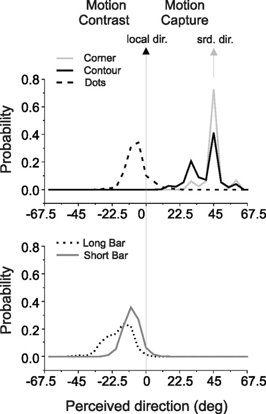
Human psychophysical results. Shown are the distributions of perceived directions for corner, contour, dot, long-bar and short-bar stimuli. Data were obtained from four subjects (G.B., X.H., M.N., and M.T.). For each stimulus condition, results from 612 to 632 trials were pooled. Data from stimuli moving in different directions were aligned so that 45° corresponds to the motion of the surround features (also the cued feature in the case of corner stimuli) (gray arrow). For all but corner stimuli, 0° corresponds to the local motion of the cued feature (black arrow). Positive angles indicate motion capture and negative angles indicate motion contrast. The top panel shows results for corner (solid gray line), contour (solid black line), and dot stimuli (dashed black line). The bottom panel shows results for long-bar (black dotted line) and short-bar (solid gray line) stimuli.

For dot stimuli, directional reports revealed motion contrast: the dots were reported to move in a direction opposite to that of the surrounding features (Fig. 2, dashed line, top). The vector-averaged angular shift was −6.6°, which was significantly different from 0° (Student's t test, p = 2.3 × 10⁻⁹³).

For short- and long-bar stimuli, psychophysical reports also indicated motion contrast. For short-bar stimuli, the vector-averaged angular shift was −9.5° (Fig. 2, gray line, bottom), which was significantly different from 0° (Student's t test, p = 0). Motion contrast for long-bar stimuli was, on average, stronger than for either dot or short-bar stimuli: the vector-averaged angular shift was −18.1° (Fig. 2, dotted line, bottom). This was significantly different from 0° (Student's t test, p = 0) and also significantly different from the −9.5° average perceptual report yielded by the short-bar stimuli (Student's t test, p = 5.9 × 10⁻⁸⁰). In conclusion, these 4 different center-surround stimuli evoked either motion contrast or motion capture.

Responses of MT neurons to contour stimuli: integrative modulation

Previous examinations of surround modulation in area MT found that surround modulation is usually antagonistic: responses were smaller when the surround portion of stimulus moved in a preferred direction (i.e., based on motion within the CRF) than when it moved in a less preferred direction (Allman et al., 1985a; Tanaka et al., 1986; Xiao et al., 1997; Bradley and Andersen, 1998). Antagonistic modulation is consistent with a perception of motion contrast (Murakami and Shimojo, 1995, 1996). We recently discovered, however, that when the CRF stimulus was one contour of a moving square that extended into the nonclassical surround (i.e., the “contour stimulus”) (Fig. 1A), surround modulation within area MT was most often “integrative” (Huang et al., 2007): responses were larger when the surround portion of stimulus moved in a preferred direction than when it moved in a less preferred direction. Integrative modulation is consistent with the perception of motion capture that is elicited by these stimuli (Fig. 2).

Figure 3 shows an example of integrative surround modulation in response to contour stimuli. Illustrated in this figure are responses to 3 of our 5 center-surround stimuli (Fig. 1A): contour, corner, and control stimuli. Neuronal responses to the four global motions of these stimuli are shown as poststimulus time histograms (PSTHs) and as vectors (black lines) in which angles indicate the direction of global motion and lengths indicate response magnitude for that direction. Determining whether surround modulation is integrative or antagonistic requires comparing directional selectivity for motion in the surround with selectivity for motion within the CRF. In this study, responses to corner stimuli provided our reference point for selectivity within the CRF (see Materials and Methods). Corner responses were used to define two types of preferred directions. The preferred directions for the global motions of our center-surround stimuli were then compared with these preferred directions to determine whether center-surround modulation was integrative or antagonistic.

The first type of preferred direction we established based on corner responses was the global direction that yielded the largest response. We refer to that direction as the P global direction. As seen in Figure 3A, this neuron's P direction is up and to the left. Due to the aperture problem (Wallach, 1935; Marr and Ullman, 1981; Adelson and Movshon, 1982; Wuerger et al., 1996), the local motion [i.e., the directional component orthogonal to the one-dimensional (1D) feature, corresponding to the motion visible within the CRF] of the CRF contour was, for this example neuron, either upward or downward. We refer to the global direction that yields the same local motion as that of the P global direction as the PP global direction. For the P direction, the local motion for this example is up. Accordingly, the PP direction is up and to the right. For the neuron illustrated in Figure 3, responses were larger when the surround portion of the contour stimulus moved in the P direction than when it moved in the PP direction (Fig. 3B), although the local motion within the CRF was identical for these two global directions. This “P>PP” selectivity for motion in the surround indicates integrative modulation.

The second type of preferred direction we established based on corner responses was the overall preferred direction. This “corner preferred direction” (Fig. 3A, blue arrow), like the preferred directions for the other center-surround stimuli (see Materials and Methods), was computed by vector-averaging of the four response vectors. Although structurally identical to Contour stimuli, Corner stimuli were positioned so that they presented unambiguous motion within the CRF. We used the corner preferred direction to define our global prediction, which is the reference point for maximum integrative modulation. For the neuron illustrated in Figure 3, the global prediction points up and to the left (slightly more upward than the P global direction). We also computed a local prediction, which is the preferred direction of the two local motions within the CRF. The local prediction was determined by comparing responses to drifting gratings moving in the two local directions. For this example neuron, responses to gratings moving upward were greater than for gratings moving downward and hence the local prediction points upward (Fig. 3D, green arrow). To determine whether surround modulation was integrative or antagonistic, we then compared the contour preferred direction (Fig. 3B, red arrow, computed by vector-averaging of the contour response vectors), with the local and global predictions (Fig. 3E). If this neuron had only been sensitive to the local motion within the CRF, the contour preferred direction should be aligned with the local prediction. Instead, the contour preferred direction is tilted toward the global prediction, thereby indicating integrative modulation. Hence, as evidenced by its responses to all four global directions of motion, as well as its responses to just P and PP directions, this neuron exhibited the same general directional preference for motion outside the CRF as it did for motion inside the CRF. This integrative surround modulation offers a solution to the aperture problem.

We classified neurons that did not respond to control stimuli as “no-control-response neurons” and those that did as “control-response neurons.” Our control stimulus is the square minus the contour centered within the CRF (the CRF contour) and hence corresponds to the portion of the contour stimulus that distinguishes the local motion of the CRF contour from the global motion of the square (see Materials and Methods). The neuron illustrated in Figure 3 was a no-control-response neuron (Fig. 3C). Our previous examination of area MT surround modulation (Huang et al., 2007) dealt only with this class of neurons.

Figure 4 shows responses from a representative control-response neuron. Like the no-control-response example in Figure 3, the contour responses of this example revealed sensitivity to the global motion of the square: responses to the P direction were larger than to the PP direction (Fig. 4B). Moreover, the contour preferred direction was also biased away from the local prediction toward the global prediction (Fig. 4E). However, unlike the example in Figure 3, this neuron responded (weakly but significantly) to control stimuli (Fig. 4C). These control responses showed the same general directional preference as seen in response to corner stimuli.

Overcoming the aperture problem by increasing sensitivity to motion in the surround

No-control-response neurons that exhibit selectivity for the global motions of contour stimuli would appear to be exhibiting nonlinear stimulus interactions since selectivity for the surround stimulus is only seen in the presence of the CRF contour (which itself provides no global motion information). Whether such global motion selectivity is due to nonlinear stimulus interactions in the case of control-response neurons is less clear, however, as many of those neurons gave directionally selective responses to control stimuli (such as seen in Fig. 4C). Since, by definition, the surround portion of the contour stimulus intruded into the CRF, the observed global motion selectivity might be consistent with purely linear stimulus interactions within the CRF. Nonlinear stimulus interactions within the CRF of area MT neurons are, however, well documented. One type of study has found that the response to two stimuli is typically less than the sum of the responses to the individually presented stimuli (Recanzone et al., 1997; Britten and Heuer, 1999) (but see Perge et al. 2005). These studies are not directly relevant to our current study as they did not focus on how nonlinear interactions overcome the aperture problem. Of more relevance are studies that have examined the directional tuning of area MT responses to “plaid patterns” (two superimposing gratings). These studies have found that some MT neurons appear to nonlinearly integrate the motions of the two component gratings (Movshon et al., 1985; Albright and Stoner, 1992; Thiele and Stoner, 2003) thereby overcoming the directional ambiguity of the individual gratings. Majaj et al. (2007) have reported, however, that non-overlapping gratings within the CRF (“pseudoplaids”) do not elicit such integrative interactions. We wondered whether the center-surround components of our stimuli (which were contiguous but not overlapping) elicited nonlinear interactions consistent with overcoming the aperture problem. More generally, we wished to identify neurons in both no-control response and control-response samples that showed global motion-selectivity that could not be explained by linear stimulus interactions.

To achieve this goal, we first consider a linear summation model:

where R is the response rate for a particular direction of global motion (θ) and for the stimulus indicated by the icon below. This model assumes that responses to contour stimuli can be modeled as the sum of the responses to two parts of the contour stimulus, namely the Control stimulus and the CRF contour. To examine the implication of this model for directional selectivity, we need to apply it to different directions of motion. In particular, this linear model (Eq. 2) predicts the following for responses to the P and PP global directions:

Although we did not record responses to the CRF contour presented alone, the CRF contour and its motion are, as described above, identical for the P and PP directions. It follows that neuronal responses to that portion of the square must also be identical for those two global directions:

This equality allows Equation 4 to be reduced to the following:

The linear summation model thus implies that the directional modulation seen for contour responses in these two directions should be equal to that seen in response to control stimuli. Accordingly, testing this prediction tells us whether any global directional selectivity seen in response to contour stimuli involves nonlinear center-surround interactions.

For the majority of our data set, the linear prediction was not valid. For 230 (including the two example neurons illustrated in Figs. 3 and 4) of the 279 neurons (82%) in our dataset, the directional selectivity defined by the difference in responses to contour stimuli moving in the P and PP directions was significantly greater than the difference in responses to the control stimuli moving in those two directions (Student's t test, p < 0.05, using a bootstrap method, see Materials and Methods). For the 230 neurons inconsistent with the linear model, 208 had interpretable surround modulation (see Materials and Methods). These neurons were composed of 97 no-control response neurons and 111 control-response neurons. Note that we did not require that these neurons exhibit integrative modulation, but only that their responses were inconsistent with the linear model. Eight-eight percent of these nonlinear neurons (i.e., 183 of 208) exhibited integrative modulation consistent with overcoming the aperture problem. Only 12% of the 208 nonlinear neurons exhibited antagonistic modulation (i.e., responses to the P direction were less than to the PP direction).

Our results thus demonstrate that regardless of whether “surround” stimuli intrude into the CRF (i.e., for both no-control and control-response neurons), the presence of the ambiguous contour amplified responses to the unambiguous motion provided by the control-portion of the contour stimulus. This enhanced selectivity was usually integrative and hence MT neurons appear able to at least partially overcome motion ambiguity within their CRF by increasing sensitivity to unambiguous motion either partially within the CRF (i.e., for control-response neurons) or outside the CRF (no-control response neurons).

Characterizing the directional tuning of surround modulation

The above analysis was restricted to examination of responses to the P and PP directions of global motion. We devised a CMI (see Materials and Methods) to quantify the sign and magnitude of surround modulation based on responses to all four global directions. This measure compares the preferred direction for a given center-surround stimulus with the local and global predictions. The local prediction is consistent with no surround modulation and the global prediction is consistent with “perfect” surround integration. More specifically, the CMI is calculated by examining the ratio between two angles. The first angle is ϕ, which is the difference between the preferred direction for a particular stimulus (such as the contour stimulus) and the local prediction. The second angle is θ, which is the angular difference between the global prediction and the local prediction. Figure 5A illustrates CMI's dependency on these two angles. A positive CMI corresponds to motion integration and a negative CMI corresponds to motion antagonism. The CMI varies linearly from −1 (maximum antagonism, in which case ϕ is equal to −θ) to 1 (maximum integration, in which case ϕ is equal to θ). Importantly, since this metric is symmetrical relative to the local prediction, if MT neurons were insensitive to the motion of the visual context, the mean of the CMI distribution should be statistically indistinguishable from zero. As discussed in Materials and Methods, we excluded neurons from CMI quantification if surround modulation could not be reliably characterized. We refer to the neurons that were not excluded as having interpretable modulation.

To further illustrate the relationship between the CMI and the underlying “raw” directional preferences and predictions, Figure 5B shows the angle ϕ (computed using the contour preferred direction) plotted as a function of θ for all neurons with interpretable modulation. Positive and negative ϕs indicate integrative and antagonistic modulation, respectively. Most points are positive and hence most neurons exhibited integrative modulation. The points that lie close to the top diagonal line (i.e., ϕ = θ) have CMIs close to 1 whereas the points that lie close to the bottom diagonal line (i.e., ϕ = −θ) have CMIs close to −1. Points both above and below the diagonals have absolute CMI values <1.

As evidenced by mean CMIs of 0.40 and 0.49 respectively, most no-control-response (n = 102) and control-response neurons (n = 148) exhibited integrative modulation in response to contour stimuli (Fig. 5C). Both of these means are significantly greater than zero (no-control-response neurons: p = 2.8 × 10⁻¹⁹; control-response neurons: p = 4.4 × 10⁻³²; Student's t tests) and hence both samples exhibited significant integrative modulation in response to contour stimuli. In our analysis of the linear summation model applied to the P and PP global directions (see above), we found that individual neurons of both samples were more directionally selective for the global motions of contour stimuli than predicted by their responses to control stimuli. This directional selectivity was largely integrative. We asked whether the integrative modulation revealed by our CMI analysis (based on all four global directions) was also larger than predicted by responses to control stimuli. We only asked this of the control-response neurons as this was obviously true for the no-control-response neurons since they did not, by definition, respond to control stimuli. To address this question, we subtracted the control responses from the contour responses, and recomputed the CMIs based on this difference. The resultant CMI distribution had a mean that was significantly positive (Fig. 5D) (mean = 0.23, Student's t test, p = 6.4 × 10⁻⁷). This result, in conjunction with our examination of the linear summation model, demonstrates that both no-control-response and control-response neurons exhibit nonlinear center interactions: Across both samples, the presence of the CRF contour amplified sensitivity to the motion of the control-portion of the contour stimulus.

The directional tuning of the surround is stimulus-specific

Our finding that contour stimuli elicit mostly integrative surround modulation appears to contradict previous investigations of MT surround modulation, which reported predominately antagonistic modulation (Allman et al., 1985a; Tanaka et al., 1986; Xiao et al., 1995; Raiguel et al., 1995). One explanation for this discrepancy is that MT surround modulation is functionally adaptive. In particular, we have hypothesized that integrative modulation serves to overcome the aperture problem. According to this hypothesis, the discrepancy between our findings and those of previous groups resulted from differences in the CRF stimuli: CRF stimuli that present the aperture problem elicit integrative modulation whereas unambiguously moving CRF stimuli elicit antagonistic modulation.

An alternative explanation for this discrepancy is that the directional tuning of the surround is in fact fixed but spatially heterogeneous (Xiao et al., 1995), perhaps with the near surround being mostly integrative and the far surround more antagonistic. Under this scenario, the differences between our findings and those of other groups is due to differences in the surround stimuli: the surround portion of our stimuli, which were generally smaller than those of previous studies, stimulated mostly integrative regions whereas the surround stimuli of other studies stimulated mostly antagonistic regions.

As a first step in the discrimination of these hypotheses, we replaced the contour within the CRF (Fig. 6A, data are from same neuron as illustrated in Fig. 3) with a circular patch of dots having the same velocity as the local motion of the contour (Fig. 6B). The motion of these dots is not ambiguous and hence there is no aperture problem for these “dot stimuli” (Fig. 1A). Based on the hypothesis that integrative modulation functions to overcome the aperture problem, we predicted that dot stimuli would not elicit integrative modulation. Conversely, if the directional tuning of the surround is fixed, dot stimuli should, like contour stimuli, elicit mostly integrative modulation.

Figure 6.

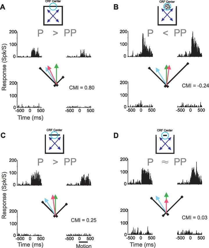
Example responses to contour, dot, and bar stimuli. Data is from same neuron as in Figure 3. Format is the same as in Figures 3, 4. Local prediction and global prediction are defined for each cell and hence the arrows depicting those predictions (green and blue arrows, respectively) are identical in these four subpanels. Qualitative relationship between responses to P and PP global directions of motion are indicated above each set of histograms. A, Responses to contour stimuli. Same data as in Figure 3B replotted to allow easy comparison with responses to dot and bar stimuli. B, Responses to dot stimuli. C, Responses to long-bar stimuli. D, Responses to short-bar stimuli. Note that the short-bar preferred direction (red arrow) was made shorter than other arrows to allow comparison with local prediction (green arrow).

As seen in Figure 6A, contour stimuli elicited integrative modulation in this example neuron: the contour preferred direction (red arrow) was biased away from the local prediction (green arrow) toward the global prediction (blue arrow). However, contrary to the hypothesis that the surround is fixed, in response to dot stimuli, this neuron exhibited antagonistic surround modulation: the dot preferred direction (i.e., the direction of the average response vector, red arrow) deviated from the local prediction (green arrow) in the direction opposite to that of the global prediction (blue arrow). The resultant CMI was −0.24. Thus, consistent with the hypothesis that surround modulation serves to overcome the aperture problem, the surround modulation of this neuron was integrative when the motion of CRF stimulus was ambiguous but antagonistic when it was not.

We tested 107 neurons with both dot and contour stimuli. Figure 7A shows the results from the 86 neurons with interpretable modulation. Whereas contour stimuli elicited mostly integrative modulation (mean CMI = 0.43, significantly positive, Student's t test, p = 1.4 × 10⁻¹⁷), dot stimuli elicited mostly antagonistic modulation (mean CMI = −0.11, significantly negative, Student's t test, p = 0.0005). Of these 86 neurons, 42 were no-control-response neurons and 44 were control-response neurons. For the 42 no-control-response neurons, the mean CMI for dot stimuli was −0.2, which is significantly negative (Student's t test, p = 3.7 × 10⁻⁵). For these neurons, the mean CMI for contour stimuli was 0.41, which is both significantly positive (Student's t test, p = 1.2 × 10⁻⁸) and significantly greater than the mean CMI to the dot stimuli (paired t test, p = 4.8 × 10⁻¹⁰).

Figure 7.

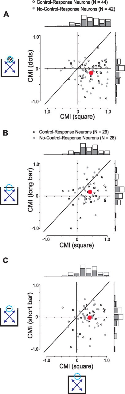
Cross-plots and marginal distributions of CMIs for contour stimuli (abscissa) and dot (A), long-bar (B), short-bar (C) stimuli (ordinates). Each point represents data from one neuron. Gray dots and gray bars indicate data from no-control response neurons. Large red dots indicate the averaged CMIs across neurons in different stimulus conditions.

Surround modulation for control-response neurons was similarly stimulus-dependent. For these neurons, the mean CMI for dot stimuli was −0.03 (not significantly different from zero; Student's t test, p = 0.5): on average, the surround stimulus had no effect on responses to the CRF contour. The mean CMI for contour stimuli was 0.44, which is both significantly positive (Student's t test, p = 1.7 × 10⁻¹⁰) and significantly greater than the mean dot-stimulus CMI (paired t test, p = 2.0 × 10⁻⁸).

Thus, most neurons of both control-response and no-control response samples, exhibited integrative modulation when the CRF stimulus was ambiguous but not when it was unambiguous. Since the portions of the surround stimuli that provided the global motion information were identical for the two stimulus types, these findings demonstrate that the integrative modulation seen for contour stimuli was not due to stimulation of surround regions with a fixed integrative influence.

The mean CMI for control-response neurons in response to dot stimuli was shifted positively relative to that of the no-control-response neurons (unpaired t test, p = 0.004). This shift toward more integrative modulation presumably reflects the fact that the control-portion of dot stimuli intruded into the CRF for control-response neurons. The directional selectivity seen in response to control stimuli generally matches that seen in response to stimuli in the CRF center (compare Figs. 4B,C) and plausibly reflects activation of feedforward inputs. Thus, a parsimonious account is that both control and no-control-response neurons exhibit antagonistic surround modulation in response to dot stimuli but that feedforward input offsets that modulation for the former sample (see below, Stimulus-dependent surround modulation: a model).

The surround portion of natural stimuli would, of course, not typically respect the CRF boundaries of MT neurons and hence the neuronal solution of the aperture problem presumably involves neurons analogous to both of these neuronal samples. Accordingly, in most of our subsequent analyses, we examine surround modulation for the two samples as a group. Since, however, the no-control response neurons correspond to those studied by us previously (Huang et al., 2007), we also offer a separate analysis of that group to allow comparison.

Does neuronal surround integration require perceptual motion capture?

The above findings are consistent with our hypothesis that surround integration serves to overcome the aperture problem. If, however, surround integration is to solve the aperture problem in a manner consistent with perception, then ambiguity within the CRF should be a necessary but not a sufficient condition: not all ambiguously moving features within the CRF should be integrated with motion in the surround. It is well established that perceptual integration of both overlapping (Adelson and Movshon, 1982; Stoner et al., 1990; Stoner and Albright, 1996) and spatially separated ambiguously moving features (Shiffrar et al., 1995; McDermott et al., 2001) is selective. For contour and dot stimuli, the presence of the aperture problem and perceptual interpretation were 100% correlated but that need not be the case.

In addition to differences in motion ambiguity and perceptual interpretation, the CRF components of contour and dot stimuli also differed in physical attributes such as spatial extent and spatial frequency content. In consequence, the presence of the aperture problem per se and/or differences in the CRF stimuli could be responsible for the differences in surround modulation seen for these two types of stimuli. To tease apart the importance of perceptual interpretation from these CRF stimulus properties, we made simple modifications of the contour stimulus, which disrupted figural continuity between the CRF and the surround stimuli. Specifically, we introduced gaps between the CRF contour and the rest of the square. These gaps were of two sizes such that the contour segment or “bar” centered within the CRF was either “long” (11.5°) (Fig. 6C) or “short” (4°) (Fig. 6D). Like the dots of the dot stimuli, these bars (including their terminators) had the same velocity as the local motion of the CRF contour in the intact square stimuli. To illustrate, for the short- and long-bar stimuli illustrated in Figure 6, if the features in the surround moved up and to the left or up and to the right, the bars moved upward; if the surround features moved down and to the left or down and to the right, the bar segment moved downward. As was true for dot and contour stimuli, the stimulus motions in the surround that distinguished Global from local predictions were identical for these three types of stimuli: long- and short-bar stimuli (illustrated in Fig. 6C,D) as well as contour stimuli.

The CRF components of these bar stimuli were only minimally different from the CRF component of contour stimuli. In fact, for neurons with CRFs small enough that the bar terminators lay outside the CRF, these CRF components were identical. In consequence, for these neurons, bar stimuli, like contour stimuli, pose the aperture problem. Unlike contour stimuli, however, bar stimuli elicit motion contrast not motion capture (Fig. 2). It follows that if we see surround integration with either of these stimuli, then surround integration would not appear to require perceptual integration (i.e., motion capture).

For the neuron illustrated in Figure 6, long-bar stimuli elicited weakly integrative modulation (Fig. 6C): responses were stronger when surround features moved up and to the left than when they moved up and to the right. This integrative modulation is revealed by the long-bar preferred direction (i.e., the average response vector, red arrow) being rotated toward the global prediction (blue arrow) and the resultant CMI of 0.25 (Fig. 6C). Although this integrative modulation was weaker than that observed for contour stimuli (Fig. 6A), these results suggest that surround integration does not require perceptual motion capture. For short-bar stimuli (Fig. 6D), this example neuron exhibited no directional modulation: responses were equally strong when the surround features moved up and to the left as when they moved up and to the right: the short-bar preferred direction (red arrow) was almost perfectly aligned with the local prediction (green arrow). The resultant CMI was 0.03.

The pattern of responses seen for this neuron mirrors that seen across the 57 neurons tested with bar and contour stimuli and which had interpretable modulation (70 neurons were tested in total). Twenty-eight of these neurons were no-control-response neurons and the other 29 were control-response neurons. Figure 7, B and C, compare CMIs for long-bar versus contour stimuli and short-bar versus contour stimuli, respectively. Each point in these figures represents the CMIs calculated from the responses of a single neuron to contour stimuli (abscissa) and to long-bar stimuli (Fig. 7B) or to short-bar stimuli (Fig. 7C) (ordinate). Gray circles represent no-control-response neurons.

For contour stimuli, the median CMI was 0.39, which was significantly greater than zero (Student's t test, p = 1.3 × 10⁻¹²) and matched that of the larger sample (Fig. 5C). For long-bar stimuli (Fig. 7B), the median CMI of 0.11 was significantly >0 for both the overall 57 neurons (Student's t test, p = 0.009) and the 28 no-control-response neurons (median = 0.16, signed-rank t test, p = 0.007). Both median CMIs were significantly smaller than those based on contour responses as indicated by the fact that most data points lay below the diagonal equality line (signed rank test, p < 0.002).

For short-bar stimuli (Fig. 7C), the median CMI is 0.0045 for the whole sample of 57 neurons and −0.011 for the 28 no-control response neurons, none was significantly different from zero (signed rank test, p > 0.8) and both were significantly smaller than those seen in response to contour stimuli (signed rank test, p < 0.0008).

In summary, for the overall neuronal sample, long-bar stimuli elicited significant integrative modulation whereas short-bar stimuli elicited no net modulation. Moreover, for both types of bar stimuli, the observed modulation was less integrative than found for contour stimuli. The long-bar results suggest that surround integration does not require perceptual integration. Given that our psychophysical data were collected from attending humans and our neurophysiological data were collected from passively fixating monkeys, this conclusion should be considered tentative (see Discussion).

Dependency of surround modulation on the aperture problem

Long-bar stimuli were more likely to extend beyond the CRFs of our sampled cells than were short-bar stimuli and hence were more likely to present the aperture problem. Accordingly, one possible explanation for our finding that long-bar stimuli elicited integrative modulation whereas short-bar stimuli did not is that integrative modulation dominates whenever the CRF stimulus is ambiguous due to the aperture problem.

To determine on a cell-by-cell basis whether bar stimuli presented the aperture problem, we devised a bar-control stimulus (Fig. 8A, bottom), which were squares with the bars deleted. These bar-control stimuli thus precisely complemented the individual bars of the short- and long-bar stimuli and moved with the same speed and in the same two directions (i.e., local not global directions) as the bars. If these stimuli elicited responses that were significantly greater than baseline, we inferred that the terminators of the corresponding bar stimulus were inside the CRF. Among the 70 neurons tested with bar stimuli, we tested 49 neurons with bar-control stimuli. If they responded to these control stimuli we classified them as not subject to the aperture problem (for that specific bar length), else they were classified as subject to the aperture problem.

For short-bar stimuli, 41 of the 49 neurons had interpretable modulation. Only seven of these 41 neurons were judged to be subject to the aperture problem for short-bar stimuli. In comparison, for long-bar stimuli, 36 of the 49 neurons had interpretable modulation and 16 of those were subject to the aperture problem. This difference in the number of neurons subject to the aperture problem for these two stimulus classes supports the hypothesis that the degree of integrative modulation depends upon whether the CRF stimulus presents the aperture problem.

We next asked whether, for a given class of stimulus (i.e., short- or long-bar stimuli), surround modulation depended upon whether the bar presented the aperture problem within the CRF. We tested two hypotheses. First, we tested the hypothesis that surround modulation was integrative for neurons subject to the aperture problem. Second, we tested the hypothesis that surround modulation was more integrative for neurons that were subject to the aperture problem than for neurons that were not.

The mean CMI for the neurons (n = 7) subject to the aperture problem for short-bar stimuli was −0.014, whereas the mean of the CMI for the neurons that were not subject to the aperture problem (n = 34) for short-bar stimuli was −0.096. Although neither of the above hypotheses was supported by the short-bar data, the sample size was too small to confidently avoid a type II error. To detect a CMI deviation from zero (i.e., hypothesis 1) the calculated powers of our t test were as follows: 0.18 for a deviation of 0.10, 0.43 for a deviation of 0.20, and 0.71 for a deviation of 0.30. To detect that the mean aperture-problem CMI was greater than the mean no-aperture-problem CMI (i.e., hypothesis 2, one-tailed) the calculated powers of our t test were: 0.175 for a deviation of 0.10, 0.41 for a deviation of 0.20, and 0.687 for a deviation of 0.30. The short-bar data were thus inconclusive.

The long-bar data supported the above hypotheses. For neurons subject to the aperture problem for long-bar stimuli (n = 16), the mean CMI was 0.24, which is significantly greater than zero (Student's t test, p = 0.026, one-sided). These neurons had smaller CRFs and were composed entirely of no-control-response neurons. Conversely, the mean CMI of the neurons that were not subject to the aperture problem (n = 20) was 0.037, which is not significantly different from 0 (Student's t test; p = 0.54). These neurons had larger CRFs and were composed of mostly control-response neurons (only two were no-control-response neurons). The mean CMI of the aperture-problem-neurons was also significantly greater than that of the no-aperture problems (two-sample, one-tailed t test, p = 0.036). Figure 8B shows these results.

Therefore, for long-bar stimuli, integrative modulation depends upon whether individual neurons were presented with the aperture problem. Given that the short-bar data were inconclusive, we take these findings as tentative support for the general hypothesis that MT neurons exhibit integrative modulation if the CRF stimulus is ambiguous due to the aperture problem.

Response magnitude and surround modulation

In our original study (Huang et al., 2007), we found that dot stimuli evoked stronger responses than did contour stimuli thus suggesting a relationship between response magnitude and surround modulation. In this study we asked whether this relationship generalized to our larger stimulus set, which included short- and long-bar stimuli, as well as contour and dot stimuli.

As one measure of response rate, we averaged the responses to the P and PP directions. Among these stimuli, contour stimuli elicited the weakest average response (22.9 and 23.5 spikes/s in the two experimental blocks, see Materials and Methods, Stimulus blocks) followed by long-bar stimuli (25.1 spikes/s), short-bar stimuli (29.6 spikes/s), and with dot stimuli (38.8 spikes/s) giving the largest average response (Fig. 9A). Across the neuronal sample, we found a significant effect of stimulus type on response magnitude (one-way ANOVA, p < 0.05). We also made pairwise comparisons in response magnitudes to stimuli that were interleaved within experimental blocks. For the experimental blocks including contour, long-bar and short-bar stimuli, pairwise comparisons of response magnitude between contour and long-bar stimuli, and between long-bar and short-bar stimuli showed a significant difference (paired t test, p < 0.01, after Bonferroni correction). For the experimental blocks including contour and dot stimuli, the response magnitude of the dot condition was significantly greater than that of the contour condition (paired t test, p < 0.001).

Figure 9.

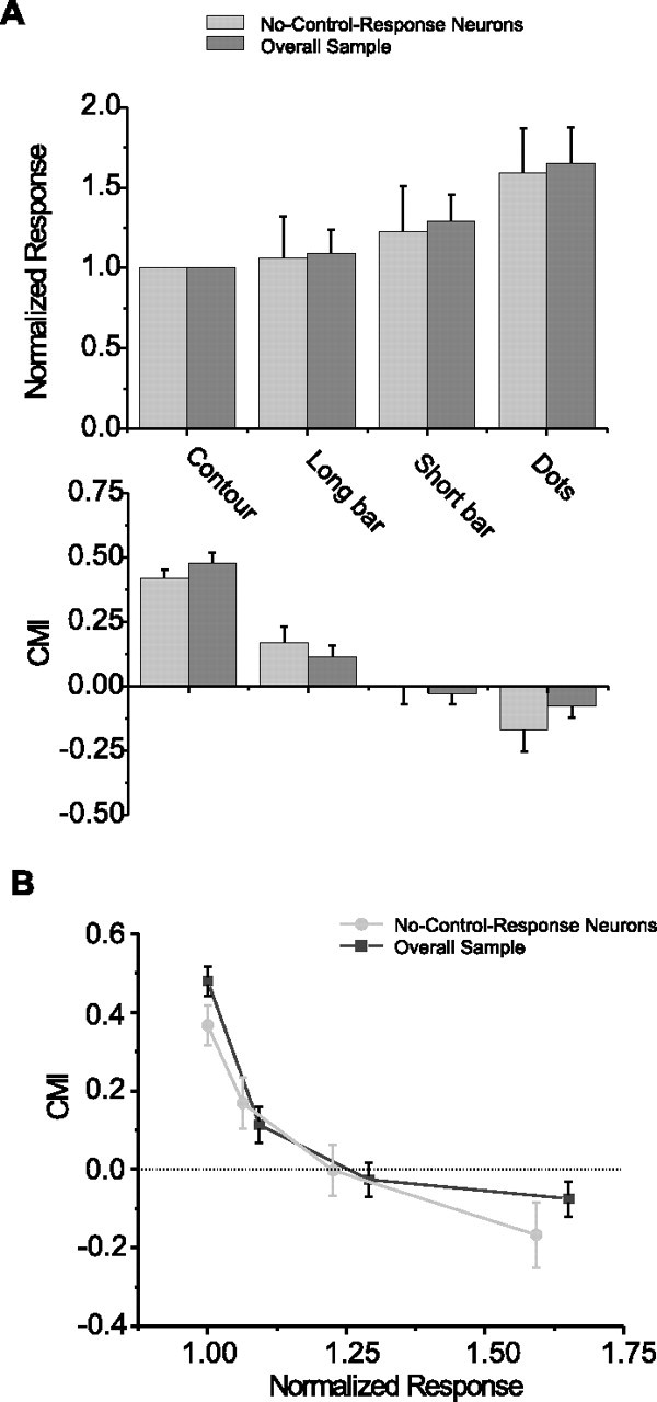
Relationship between firing rate and surround modulation. A, Top panel shows the averaged response to the P and the PP directions across neurons in the contour, long-bar, short-bar, and dot conditions. Response magnitude was normalized to maximum response to contour stimuli. Bottom panel shows averaged CMIs in these stimulus conditions. Dark gray bars depict results from the overall sample (N = 208 for contour stimuli; N = 57 for long-bar and short-bar stimuli; N = 86 for dot stimuli), and light gray bars depict results from no-control response neurons (N = 97 for contour stimuli; N = 28 for long-bar and short-bar stimuli; N = 42 for dot stimuli). Error bars indicate SE. B, Cross-plot of CMI as a function of normalized response magnitude. As the response magnitude increases (across stimulus conditions), the average CMI decreases and changes from integrative to antagonistic.

The ordering of stimuli as a function of response magnitude held up regardless of whether response magnitude was based on the averaged response to the P and PP global directions (Fig. 9A, top), the averaged response to the four global directions, or the maximum response. This trend also held for both the whole sample (Fig. 9A, dark gray columns) and the no-control response sample (Fig. 9A, light gray columns). The CMIs based on the responses to these stimulus types exhibited an opposite trend: The larger the average response, the less integrative and/or more antagonistic was surround modulation (Fig. 9A, bottom). Figure 9B shows the relationship between CMI and response magnitude.

Stimulus-dependent surround modulation: a model

The observed relationship between the directional tuning of surround modulation and firing rate recalls the finding by Pack et al. (2005) that increasing the size of a high-contrast stimulus beyond a certain point elicits suppression whereas increasing the size of a low-contrast stimulus to the same extent results in a response increase (see Tadin et al. 2003, for apparent perceptual consequences that may be related to this suppression). Since firing rate also covaried with luminance contrast, that study also demonstrated a relationship between firing rate and surround modulation [although Pack et al. (2005) did not examine the directional selectivity of the modulation they observed]. Somers et al. (1998) have shown that a simple circuit incorporating known patterns of connectivity can account for such contrast-dependent effects in area V1.

We developed a simple neural network model that reproduces the relationship between firing rate and surround modulation discovered in this study. This model also reproduces the contrast-dependent modulation observed by Pack et al. (2005). In our model, we assume that surround inhibition and excitation are directionally tuned and mediated by horizontal connections between adjacent hypercolumns within area MT (Fig. 10A). A key assumption, consistent with the model of Somers et al. (1998), is that lateral inhibition grows faster than lateral excitation as the strength of feedforward input grows. In other words, input strength shifts the balance between directionally tuned lateral excitation and inhibition, thus determining both the strength and the “sign” (i.e., whether integrative or antagonistic) of surround modulation. As a result of this dependency, facilitation and integration yield to suppression and antagonism as the strength of the input increases. This property arises from two features of our model. First, lateral excitation is mediated directly by connections between excitatory neurons, whereas lateral inhibition is mediated indirectly via inhibitory interneurons. Second, consistent with known anatomy of area MT (Anderson et al., 1998), both excitatory and inhibitory neurons receive excitatory feedforward input. We have assumed that the differences in firing rate we have observed are, on average, monotonically related to the strength of the feedforward input provided to both excitatory and inhibitory neurons. Accordingly, we examine the relationship between firing rate and surround modulation by varying input strength to both types of neurons.

Figure 10.

Model of input-dependent surround modulation. A, Two directional columns within adjacent “center” and “surround” hypercolumns. Each column consists of an excitatory (E) and an inhibitory (I) neuron. Excitatory and inhibitory neurons receive feedforward input from V1. Lateral excitation (•) between hypercolumns occurs via direct connections between excitatory neurons. Lateral inhibition (○) is mediated via inhibitory interneurons. The level of feedforward input into the inhibitory neurons determines the efficacy of lateral inhibition. All connections are symmetrical so center and surround designations are arbitrary. B, Directional weighting of connections. Center and surround hypercolumns each consist of 8 excitatory (bottom) and 8 inhibitory (top) neurons. Redundant types of connections are omitted to avoid clutter. In particular, the pattern of feedforward inputs to center and surround hypercolumns (i.e., W_fi and W_fe) is identical but only the former are shown. Similarly, connections between hypercolumns (W_ei and W_ee) are symmetrical but are only those from the surround to the center are shown. Last, both hypercolumns have within-hypercolumn inhibition (W_ie), but this is only shown for the surround hypercolumn. The feedforward connections to inhibitory neurons (W_fi) are not directionally weighted but all other weights are. Compare with A. C, Stimulus-dependent surround integration/antagonism. Inset, Directional tuning curve for a grating within the CRF. For this model neuron, P and PP directions are up to the left and up to the right, respectively (compare with Fig. 6). In this simulation, we compare responses to surround stimuli moving in the P and PP directions while the center stimulus moves upward (i.e., the local direction within the CRF). We examined these responses as we varied the level of the “V1” input into the center hypercolumn. With no center input, the surround stimulus has no effect and hence this model neuron would be classified as a no-control-response neuron. With maximum input spike rates of 20 and 40 spikes/s, the model reproduces surround integration like that seen in area MT neurons responding to contour and long-bar stimuli, respectively (compare with Fig. 6A,C). With an input rate of 60 spikes/s, surround modulation is absent as seen in response to short-bar stimuli (compare with Fig. 6D). With higher input rates of 80 and 100, antagonistic modulation emerges consistent with responses to dot stimuli (compare with Fig. 6B). Note that this neuron exhibits supersaturation, a property that may account for the finding that some neurons do not respond more to stimuli that elicit antagonism than to stimuli that elicit integration. The polar-plots above the Cartesian plot show responses to P and PP directions for a subset of the input values. D, Contrast-dependent suppression/facilitation. For low-contrast stimuli, increasing the size of a stimulus (moving in a neuron's preferred direction) so that it stimulates the surround results in facilitation. For high-contrast stimuli, the same size increase results in surround suppression. Contrast level was implemented by varying the strength of feedforward input.

Our spike-rate equation for excitatory neurons is as follows:

R is firing rate and is determined by the hyperbolic ratio equation of Naka and Rushton (1966) applied to positive input values (shown within the brackets and indicated by + subscript). Subscripted Ws indicate synaptic weights between excitatory (e), inhibitory (i), and V1 (f) neurons, with first and second subscripts referring to presynaptic and postsynaptic neurons, respectively. The spike-rate equation for inhibitory neurons is essentially the same except that different weights are used (inhibitory weights are zero). Base is the baseline firing rate and was set to 0 and 12 for excitatory and inhibitory neurons, respectively. The nonzero baseline of the inhibitory neuron insures that small excitatory inputs from the surround fail to elicit a response in the excitatory neurons they inhibit. This reproduces the behavior of a no-control-response neuron. Smaller baseline rates yield behavior like that of control-response neurons. Max is the maximum firing rate and was set to 100 and 150 spikes/s for excitatory and inhibitory neurons respectively. S is the input level that leads to a response that is halfway between the baseline and maximum firing rates, and was set to 40 and 80 spikes/s for excitatory and inhibitory neurons, respectively. Last, the exponent N dictates the maximum slope of the activation function, and was set to 3 and 4 for excitatory and inhibitory neurons, respectively. Consistent with experimental findings (Connors et al., 1982; McCormick et al., 1985; Nowak et al., 2003), these parameters impart higher maximum firing rates and larger maximum gains (i.e., steeper functions) for inhibitory neurons relative to excitatory neurons. In addition, inhibitory neurons require stronger input than excitatory neurons before they reach the steep portion of their activation function.

We can achieve qualitatively similar results with other parameters that preserve these qualitative differences between excitatory and inhibitory neurons, as well with different activation functions (such as an exponential with a threshold parameter).

As indicated above, the dependency of surround modulation on input strength in this model arises because the inhibitory neurons have nonlinear input–output functions and receive feedforward as well as lateral input. The feedforward input, in effect, determines the gain of surround suppression. For low feedforward inputs, inhibitory neurons operate in the shallow-slope (low-gain) region of their input–output curve and hence a given input from the excitatory neuron in the surround has minimal impact on the firing rate of the inhibitory neuron. For higher inputs, however, inhibitory neurons operate in the steep (high-gain) region of their input–output curve: the same surround input that had minimal impact under low-feedforward conditions now evokes a large change in the firing rate of the inhibitory neuron. Conversely, since lateral excitation is direct, the strength of excitatory input is not dependent upon the input level into the center hypercolumn. In consequence, the balance between lateral excitation and inhibition changes in favor of inhibition as the input into the center hypercolumn increases. This behavior reproduces contrast-dependent surround modulation by Pack et al. (2005) (see below).

While the two design features referred to above can account for contrast-dependent shifts in surround suppression and facilitation, to account for the directionally tuned effects reported here, our model also assumes that lateral excitation and inhibition are directionally tuned. Our full model consists of one center and one surround directional hypercolumn, each with 8 excitatory and 8 inhibitory neurons (Fig. 10B). Feedforward input (from “area V1”) consists of 8 matching units per hypercolumn, each with a von Mises direction-tuning function:

R is the response rate for a particular direction of motion (θ) and PD is the preferred direction of the model neuron. For these simulations: A = 10; B = 15; C = 60.

With the exception of feedforward input to the inhibitory neurons (see below), neuronal connectivity is directionally tuned:

This formula applies to 4 of 5 of the synaptic weights in our model: W_fe, W_ie, W_ee, and W_ei. W_max is the maximum weight for each of these four corresponding synapse types: 0.19, 0.30, 0.14, and 0.22. PD_dif is the difference in the preferred directions of the presynaptic and postsynaptic neurons. The synaptic weight (W_fi) of the feedforward input onto the inhibitory neurons is not directionally tuned (i.e., it is the same from all input neurons) and was set to 0.075. W_fi's lack of directional tuning reproduces the finding that the tuning of surround suppression does not depend upon the particular direction of motion of the center stimulus (Born, 2000). We also found empirically that modulatory effects were larger if W_fi were untuned rather than having the same tuning as the other weights. It is interesting to note that other groups have also invoked untuned cortical inhibition but have done so based on quite different stimulus-tuning and contrast-invariance arguments (Somers et al., 1995; Troyer et al., 1998; Lauritzen and Miller, 2003; Ringach et al., 2003).

Figure 10C illustrates the behavior of an excitatory model neuron within the center hypercolumn that prefers motion up and to the left. We examine responses to the P and PP global directions as selectivity for these two directions provides a simple and intuitive measure of whether surround modulation is integrative or antagonistic. The center stimulus moved upward (i.e., 45 degrees away from the preferred direction) and surround stimuli moved in either the P direction (i.e., up and to the left) or in the PP direction (i.e., up and to the right). To examine the influence of input strength into the center hypercolumn, we held the level of input to the surround hypercolumn constant (i.e., we held the maximum firing rate of the V1 input to 100 spikes/s) and varied the center input by scaling V1 firing rates. This manipulation was meant to mimic our experimental manipulations in which we kept the key surround features (i.e., the control stimulus) constant but varied the CRF stimulus. In the absence of V1 input into the center hypercolumn, surround stimuli do not evoke responses. For the lowest nonzero input (i.e., 20 spikes/s max V1 firing rate), surround stimuli evoke direction-selective responses and that selectivity reflects integrative surround modulation: a surround stimulus moving in the P direction results in a larger response than does one moving in the PP direction.

This behavior is similar to that we observed in response to contour stimuli (Fig. 6A). Increasing the input strength slightly (40 spikes/s maximum V1 input) yields integrative modulation that is somewhat smaller than that seen for the lowest level of input. This behavior is analogous to that seen in response to long-bar stimuli (compare with Fig. 6C). Increasing the V1 input level to 60 spikes/s results in no directional modulation, resembling responses to short-bar stimuli (compare with Fig. 6D). With higher input rates of 80 and 100, antagonistic modulation emerges consistent with responses to dot stimuli (compare with Fig. 6B). Note that this model neuron exhibits supersaturation (Maffei and Fiorentini, 1973; Albrecht and Hamilton, 1982; Li and Creutzfeldt, 1984), a property that can account for the finding that not all neurons in our sample responded more to stimuli that elicit antagonism than to stimuli that elicit integration. The model of Somers et al. (1998) also reproduced this response property of supersaturation.

Figure 10D illustrates the behavior of the same model neuron illustrated in Figure 10C when stimulated with low- and high-contrast stimuli (simulated by adjusting the maximum firing rate of the V1 inputs to 16 and 50 spikes/s, respectively). For these two levels of input magnitude, we compare the responses of a model excitatory neuron to a stimulus moving in its preferred direction positioned in the center of the CRF (i.e., “C”) to that stimulus plus a surround stimulus also moving in that preferred direction (i.e., “C + S”). For low-contrast stimuli, addition of the surround stimulus results in an increase in response, whereas, for high-contrast stimuli, addition of the surround stimulus results in a substantial reduction of firing rate. This behavior qualitatively matches that of real MT neurons [compare with Pack et al. (2005), their Fig. 1A].

Our model thus offers a critical link between our results, which demonstrate shifts in the directional tuning of surround modulation in area MT, and the findings of Pack et al. (2005), which demonstrate contrast-dependent shifts in surround suppression. These two types of stimulus-dependent shifts in surround modulation have yet to be studied in tandem and our model offers a key prediction: the directional tuning of surround modulation should transition from antagonistic to integrative as the luminance contrast of the CRF stimulus goes from high to very low. For example, the high-contrast dot stimuli used by Pack et al. (2005) should yield antagonistic modulation whereas their low-contrast stimuli should yield integrative modulation.

Finally we note that Guo et al. (2006) have reported that some neurons in area V1 may be able to overcome the aperture problem via surround modulation. Although Guo et al. did not ask whether that modulation was stimulus specific, it is tempting to speculate that circuitry like that proposed here also exists in area V1. However, given the relatively small spatial scale and magnitude of the effects reported by Guo et al. (2006), we think it unlikely that the area MT surround effects documented in our study reflect properties inherited from area V1 (see also Pack et al. 2005).

Discussion

We found that MT surround modulation was stimulus-dependent, ranging from antagonistic to integrative. Surround modulation matched perceptual interpretation (assayed in humans) under some conditions but not others. Specifically, motion ambiguity within the CRF appeared to be a better predictor of surround modulation than perceptual interpretation: stimuli that presented ambiguous motion within the CRF elicited surround integration although their perceptual interpretation was consistent with surround antagonism. We found, moreover, that the directional tuning of surround modulation was related to how well stimuli drove MT responses. We developed a neural network model that accounted for that relationship. We discuss these results in the context of previous findings and speculate about the implications of these results with regard to the neuronal mechanisms underlying contextual interactions.

Surround modulation: suppression, facilitation, antagonism, and integration

Stimuli outside the CRF do not, by definition, yield a response, but they can modulate responses to stimuli within the CRF (Born, 2000) (for review, see Allman et al., 1985b; Gilbert, 1992; Fitzpatrick, 2000; Albright and Stoner, 2002). This modulation can be characterized along two dimensions: (1) suppression/facilitation and (2) antagonism/integration. Suppression and facilitation refer to decreases and increases, respectively, in neuronal response upon addition of a surround stimulus to a CRF stimulus. Antagonism and integration, however, refer to surround modulation tuning that opposes or matches, respectively, that of the CRF. Our study investigated this latter dimension of surround modulation. In particular, we tested the hypothesis that surround modulation in area MT could function to overcome the aperture problem.

The aperture problem and MT surround modulation: previous studies

Motion parallel to a 1D feature, such as a contour, is invisible and hence the motion of a 1D feature is indeterminate. Conversely, two-dimensional (2D) features, such as corners, provide unambiguous motion information. At the neuronal level, the aperture problem arises when only a 1D feature is present in the CRF. To overcome ambiguity within the CRF, surround modulation needs to be integrative: the addition of a surround stimulus moving in the preferred direction of the cell, should, like CRF stimuli, yield larger responses relative to a surround stimulus moving in a less preferred direction. Based on previous reports that the directional tuning of surround modulation within MT (Allman et al., 1985a; Tanaka et al., 1986; Xiao et al., 1997; Bradley and Andersen, 1998) is generally antagonistic, one might assume that the aperture problem is not solved via surround modulation.

Duncan et al. (2000) were the first to report that MT neurons could overcome the aperture problem via surround modulation but the design of their experiments did not allow characterization of surround modulation as antagonistic or integrative. Huang et al. (2007) confirmed that area MT neurons could overcome the aperture problem via surround modulation and, more importantly, found that this was accomplished via adaptive changes in the directional tuning of surround modulation. Their findings were moreover consistent with previous evidence that area MT underlies the selective perceptual integration/segmentation of moving features (Stoner and Albright, 1992; Duncan et al., 2000; Thiele and Stoner, 2003).

A dissociation between surround modulation and perception?

In the present study, we found evidence of dissociation between perception and neuronal responses: stimuli that elicited motion contrast perceptually elicited surround integration neuronally if they presented ambiguous motion within the CRF. These results are, to our knowledge, the first evidence of area MT neurons that do the opposite of what perceptual reports predict. Given however that the monkeys in our study did not provide perceptual reports, we cannot draw firm conclusions about the relationship between perception and neuronal responses. Before considering why perception might differ between our monkey and human subjects, we consider what our findings tell us about the functions and mechanisms underlying surround modulation in area MT.

The role of input strength in surround modulation

We found that the directional tuning of surround modulation was systematically related to the level of response elicited. These findings have mechanistic and functional implications. Mechanistically, we found that our results are consistent with a circuit in which the balance between antagonism and integration is determined by input strength. This circuit also accounts for contrast-dependent effects of surround modulation in area MT (Pack et al., 2005) and is similar in design to that shown to account for such effects in area V1 (Somers et al., 1998). This modeling work raises the attractive possibility that a simple canonical circuit might explain seemingly diverse neuronal properties in different cortical areas.

The functional implication of our findings follows from the observation that response magnitude under many conditions appears to reflect sensory reliability: high-contrast stimuli offer more reliable motion estimates than do low-contrast stimuli, and 2D features provide more reliable motion estimates than do 1D features (Weiss et al., 2002). This reliability is mirrored by response magnitude in area MT: high-contrast stimuli typically yield larger responses than low-contrast stimuli in area MT (Pack et al., 2005) and 2D features generally yield larger responses than 1D features in MT (Pack et al., 2004). This relationship suggests that the adaptive changes in surround modulation observed in area MT may therefore reflect, in part, adaptive responses to directional uncertainty (Huang et al., 2007). It may nevertheless be true that the relationship between stimulus strength and ambiguity proposed here does not generally hold. Experiments that couple behavioral measurements of uncertainty with in-tandem measurements of neuronal response levels are needed if this relationship is to be tested more rigorously.

Our findings suggest that (under the conditions of our experiments) surround modulation in area MT is governed by simple local principles, both functionally and mechanistically. These simple principles appear insufficient, however, to account for the fact that perceptual interactions between moving features can, under many conditions, be rather sophisticated (Stoner et al., 1990; Shiffrar et al., 1995; Duncan et al., 2000). Indeed, we found that CRF ambiguity and firing rate appeared to be a better predictor than perceptual interpretation. We next address the apparent discrepancy between surround modulation and perception.

Attention and center-surround interactions

The monkeys in our experiments may have perceived our stimuli differently than our human subjects. One basis for such a discrepancy is the difference in attentional requirements: human subjects were required to attend to these stimuli (to make directional judgments), whereas monkeys were only required to fixate. It may be that our findings (and our model) capture the behavior of area MT only when attention is withdrawn. Surround modulation in MT may, like perception, be more sophisticated when attention is directed to the stimulus in question. The finding that attention changes the receptive field profiles of area MT neurons is consistent with such speculation (Womelsdorf et al., 2006).

Attention has been previously implicated in both motion contrast and motion capture. In particular, attending to one of two motions within the CRF has been found to reduce the inhibitory influence of the second motion (Treue and Maunsell, 1996, 1999). This decrease in directional interaction agrees with the psychophysical results of Chen et al. (2005) who found that attending to one of two superimposed moving stimuli, reduced repulsion (i.e., motion contrast) between them.

Culham and Cavanagh (1994) have proposed that motion capture depends upon attention (but see Ramachandran, 1996). This proposition, however, runs opposite to the discrepancy we report: we found stimulus conditions that elicited surround integration (consistent with motion capture) in monkeys that were presumably not attending these stimuli, whereas human subjects, who attended those stimuli, reported motion contrast. The role of attention in our findings thus remains unclear.

If the perceptions of our monkeys were in fact the same as our human subjects, this would suggest that MT does not directly underlie the perception of these stimuli. Conversely, there could be intrinsic differences in the way these two species perceive these stimuli. Given previous evidence that macaque monkeys perceptually segment and integrate moving features similarly to humans (Thiele and Stoner, 2003; Zivotofsky et al. 2005), we think that possibility unlikely. Distinguishing between these possibilities requires that behavioral responses be collected simultaneously with neuronal responses.

While a perceptual mismatch between our human and monkey subjects is plausible, such a mismatch cannot fully explain our results. This is because the qualitative dissociation we observed between neuronal and perceptual responses was only found for neurons with small enough CRFs that they were subject to the aperture problem. Thus, no matter how the monkeys in our experiments perceived these stimuli, our findings demonstrate that the relationship between MT neuronal responses and perception was not uniform.

Conclusion

We found that the directional tuning of surround modulation is stimulus-dependent. A key finding was that the directional tuning of surround modulation depends upon motion ambiguity: stimuli that presented ambiguous motion within the CRF elicited integrative modulation whereas those that presented unambiguous motion within the CRF elicited either antagonistic modulation or no directional modulation. Moreover, we found that the tuning of surround modulation is also related to stimulus strength (how well stimuli drive neuronal responses) and developed a simple neural network model that accounts for that relationship. We hypothesize that ambiguous stimuli provide weak input to MT and elicit surround integration whereas unambiguous stimuli provide strong input to MT and elicit surround antagonism. We also found a partial disagreement between perceptual reports (of human subjects) and neuronal responses. Determining whether this dissociation extends to monkey perception will be addressed in future experiments in which perceptual as well as neuronal responses are recorded from monkeys. Together, our results suggest that, under the conditions of our experiment, stimulus-dependent changes in MT surround modulation result from shifts in the balance between directionally tuned excitation and inhibition mediated by changes in input strength. Our findings highlight the importance of not assuming that neuronal responses properties observed under one set of stimulus conditions generalize to other conditions.

References

- Adelson EH, Movshon JA. Phenomenal coherence of moving visual patterns. Nature. 1982;300:523–525. doi: 10.1038/300523a0. [DOI] [PubMed] [Google Scholar]
- Albrecht DG, Hamilton DB. Striate cortex of monkey and cat: contrast response function. J Neurophysiol. 1982;48:217–237. doi: 10.1152/jn.1982.48.1.217. [DOI] [PubMed] [Google Scholar]
- Albright TD, Stoner GR. Contextual influences on visual processing. Annu Rev Neurosci. 2002;25:339–379. doi: 10.1146/annurev.neuro.25.112701.142900. [DOI] [PubMed] [Google Scholar]
- Allman J, Miezin F, McGuinness E. Direction- and velocity-specific responses from beyond the classical receptive field in the middle temporal visual area (MT) Perception. 1985a;14:105–126. doi: 10.1068/p140105. [DOI] [PubMed] [Google Scholar]
- Allman J, Miezin F, McGuinness E. Stimulus specific responses from beyond the classical receptive field: neurophysiological mechanisms for local-global comparisons in visual neurons. Annu Rev Neurosci. 1985b;8:407–430. doi: 10.1146/annurev.ne.08.030185.002203. [DOI] [PubMed] [Google Scholar]
- Anderson JC, Binzegger T, Martin KA, Rockland KS. The connection from cortical area V1 to V5: a light and electron microscopic study. J Neurosci. 1998;18:10525–10540. doi: 10.1523/JNEUROSCI.18-24-10525.1998. [DOI] [PMC free article] [PubMed] [Google Scholar]
- Born RT. Center-surround interactions in the middle temporal visual area of the owl monkey. J Neurophysiol. 2000;84:2658–2669. doi: 10.1152/jn.2000.84.5.2658. [DOI] [PubMed] [Google Scholar]
- Braddick O. Segmentation versus integration in visual motion processing. Trends Neurosci. 1993;16:263–268. doi: 10.1016/0166-2236(93)90179-p. [DOI] [PubMed] [Google Scholar]
- Bradley DC, Andersen RA. Center-surround antagonism based on disparity in primate area MT. J Neurosci. 1998;18:7552–7565. doi: 10.1523/JNEUROSCI.18-18-07552.1998. [DOI] [PMC free article] [PubMed] [Google Scholar]
- Chang JJ, Julesz B. Cooperative phenomena in apparent movement perception of random-dot cinematograms. Vision Res. 1984;24:1781–1788. doi: 10.1016/0042-6989(84)90009-9. [DOI] [PubMed] [Google Scholar]
- Chen Y, Meng X, Matthews N, Qian N. Effects of attention on motion repulsion. Vision Res. 2005;45:1329–1339. doi: 10.1016/j.visres.2004.11.005. [DOI] [PubMed] [Google Scholar]
- Connors BW, Gutnick MJ, Prince DA. Electrophysiological properties of neocortical neurons in vitro. J Neurophysiol. 1982;48:1302–1320. doi: 10.1152/jn.1982.48.6.1302. [DOI] [PubMed] [Google Scholar]
- Culham JC, Cavanagh P. Motion capture of luminance stimuli by equiluminous color gratings and by attentive tracking. Vision Res. 1994;34:2701–2706. doi: 10.1016/0042-6989(94)90226-7. [DOI] [PubMed] [Google Scholar]
- Duncan RO, Albright TD, Stoner GR. Occlusion and the interpretation of visual motion: perceptual and neuronal effects of context. J Neurosci. 2000;20:5885–5897. doi: 10.1523/JNEUROSCI.20-15-05885.2000. [DOI] [PMC free article] [PubMed] [Google Scholar]
- Duncker K. Source book of gestalt psychology. London: Kegan Paul, Trench, Trubner and Co; 1938. [Google Scholar]
- Fitzpatrick D. Seeing beyond the receptive field in primary visual cortex. Curr Opin Neurobiol. 2000;10:438–443. doi: 10.1016/s0959-4388(00)00113-6. [DOI] [PubMed] [Google Scholar]
- Gilbert CD. Horizontal integration and cortical dynamics. Neuron. 1992;9:1–13. doi: 10.1016/0896-6273(92)90215-y. [DOI] [PubMed] [Google Scholar]
- Guo K, Robertson R, Nevado A, Pulgarin M, Mahmoodi S, Young MP. Primary visual cortex neurons that contribute to resolve the aperture problem. Neuroscience. 2006;138:1397–1406. doi: 10.1016/j.neuroscience.2005.12.016. [DOI] [PubMed] [Google Scholar]
- Huang X, Albright TD, Stoner GR. Adaptive surround modulation in cortical area MT. Neuron. 2007;53:761–770. doi: 10.1016/j.neuron.2007.01.032. [DOI] [PMC free article] [PubMed] [Google Scholar]
- Krekelberg B, Albright TD. Motion mechanisms in macaque MT. J Neurophysiol. 2005;93:2908–2921. doi: 10.1152/jn.00473.2004. [DOI] [PubMed] [Google Scholar]
- Lauritzen TZ, Miller KD. Different roles for simple-cell and complex-cell inhibition in V1. J Neurosci. 2003;23:10201–10213. doi: 10.1523/JNEUROSCI.23-32-10201.2003. [DOI] [PMC free article] [PubMed] [Google Scholar]
- Li CY, Creutzfeldt O. The representation of contrast and other stimulus parameters by single neurons in area 17 of the cat. Pflugers Arch. 1984;401:304–314. doi: 10.1007/BF00582601. [DOI] [PubMed] [Google Scholar]
- Maffei L, Fiorentini A. The visual cortex as a spatial frequency analyser. Vision Res. 1973;13:1255–1267. doi: 10.1016/0042-6989(73)90201-0. [DOI] [PubMed] [Google Scholar]
- Majaj NJ, Carandini M, Movshon JA. Motion integration by neurons in macaque MT is local, not global. J Neurosci. 2007;27:366–370. doi: 10.1523/JNEUROSCI.3183-06.2007. [DOI] [PMC free article] [PubMed] [Google Scholar]
- Marr D, Ullman S. Directional selectivity and its use in early visual processing. Proc R Soc Lond B Biol Sci. 1981;211:151–180. doi: 10.1098/rspb.1981.0001. [DOI] [PubMed] [Google Scholar]
- McCormick DA, Connors BW, Lighthall JW, Prince DA. Comparative electrophysiology of pyramidal and sparsely spiny stellate neurons of the neocortex. J Neurophysiol. 1985;54:782–806. doi: 10.1152/jn.1985.54.4.782. [DOI] [PubMed] [Google Scholar]
- McDermott J, Weiss Y, Adelson EH. Beyond junctions: nonlocal form constraints on motion interpretation. Perception. 2001;30:905–923. doi: 10.1068/p3219. [DOI] [PubMed] [Google Scholar]
- Moulden B, Kingdom F, Gatley LF. The standard deviation of luminance as a metric for contrast in random-dot images. Perception. 1990;19:79–101. doi: 10.1068/p190079. [DOI] [PubMed] [Google Scholar]
- Movshon JA, Adelson EA, Gizzi M, Newsome WT. The analysis of moving visual patterns. In: Chagas C, Gattass R, Gross CG, editors. Study group on pattern recognition mechanisms. Vatican City: Pontifica Academia Scientiarum; 1985. pp. 117–151. [Google Scholar]
- Murakami I, Shimojo S. Modulation of motion aftereffect by surround motion and its dependence on stimulus size and eccentricity. Vision Res. 1995;35:1835–1844. doi: 10.1016/0042-6989(94)00269-r. [DOI] [PubMed] [Google Scholar]
- Murakami I, Shimojo S. Assimilation-type and contrast-type bias of motion induced by the surround in a random-dot display: evidence for center-surround antagonism. Vision Res. 1996;36:3629–3639. doi: 10.1016/0042-6989(96)00094-6. [DOI] [PubMed] [Google Scholar]
- Naka KI, Rushton WA. S-potentials from luminosity units in the retina of fish (Cyprinidae) J Physiol. 1966;185:587–599. doi: 10.1113/jphysiol.1966.sp008003. [DOI] [PMC free article] [PubMed] [Google Scholar]
- Nowak LG, Azouz R, Sanchez-Vives MV, Gray CM, McCormick DA. Electrophysiological classes of cat primary visual cortical neurons in vivo as revealed by quantitative analyses. J Neurophysiol. 2003;89:1541–1566. doi: 10.1152/jn.00580.2002. [DOI] [PubMed] [Google Scholar]
- Pack CC, Gartland AJ, Born RT. Integration of contour and terminator signals in visual area MT of alert macaque. J Neurosci. 2004;24:3268–3280. doi: 10.1523/JNEUROSCI.4387-03.2004. [DOI] [PMC free article] [PubMed] [Google Scholar]
- Pack CC, Hunter JN, Born RT. Contrast dependence of suppressive influences in cortical area MT of alert macaque. J Neurophysiol. 2005;93:1809–1815. doi: 10.1152/jn.00629.2004. [DOI] [PubMed] [Google Scholar]
- Perge JA, Borghuis BG, Bours RJ, Lankheet MJ, van Wezel RJ. Temporal dynamics of direction tuning in motion-sensitive macaque area MT. J Neurophysiol. 2005;93:2104–2116. doi: 10.1152/jn.00601.2004. [DOI] [PubMed] [Google Scholar]
- Raiguel S, Van Hulle MM, Xiao DK, Marcar VL, Orban GA. Shape and spatial distribution of receptive fields and antagonistic motion surrounds in the middle temporal area (V5) of the macaque. Eur J Neurosci. 1995;7:2064–2082. doi: 10.1111/j.1460-9568.1995.tb00629.x. [DOI] [PubMed] [Google Scholar]
- Ramachandran VS. Motion capture and visual attention: comments on Culham and Cavanagh (1994) Vision Res. 1996;36:77–80. doi: 10.1016/0042-6989(95)94094-v. [DOI] [PubMed] [Google Scholar]
- Ramachandran VS, Cavanagh P. Motion capture anisotropy. Vision Res. 1987;27:97–106. doi: 10.1016/0042-6989(87)90146-5. [DOI] [PubMed] [Google Scholar]
- Recanzone GH, Wurtz RH, Schwartz U. Responses of MT and MST neurons to one and two moving objects in the receptive field. J Neurophysiol. 1997;78:2904–2915. doi: 10.1152/jn.1997.78.6.2904. [DOI] [PubMed] [Google Scholar]
- Ringach DL, Hawken MJ, Shapley R. Dynamics of orientation tuning in macaque V1: the role of global and tuned suppression. J Neurophysiol. 2003;90:342–352. doi: 10.1152/jn.01018.2002. [DOI] [PubMed] [Google Scholar]
- Schoppmann A, Hoffmann KP. Continuous mapping of direction selectivity in the cat's visual cortex. Neurosci Lett. 1976;2:177–181. doi: 10.1016/0304-3940(76)90011-2. [DOI] [PubMed] [Google Scholar]
- Shiffrar M, Li X, Lorenceau J. Motion integration across differing image features. Vision Res. 1995;35:2137–2146. doi: 10.1016/0042-6989(94)00299-1. [DOI] [PubMed] [Google Scholar]
- Somers DC, Nelson SB, Sur M. An emergent model of orientation selectivity in cat visual cortical simple cells. J Neurosci. 1995;15:5448–5465. doi: 10.1523/JNEUROSCI.15-08-05448.1995. [DOI] [PMC free article] [PubMed] [Google Scholar]
- Somers DC, Todorov EV, Siapas AG, Toth LJ, Kim DS, Sur M. A local circuit approach to understanding integration of long-range inputs in primary visual cortex. Cereb Cortex. 1998;8:204–217. doi: 10.1093/cercor/8.3.204. [DOI] [PubMed] [Google Scholar]
- Stoner GR, Albright TD. Neural correlates of perceptual motion coherence. Nature. 1992;358:412–414. doi: 10.1038/358412a0. [DOI] [PubMed] [Google Scholar]
- Stoner GR, Albright TD. The interpretation of visual motion: evidence for surface segmentation mechanisms. Vision Res. 1996;36:1291–1310. doi: 10.1016/0042-6989(95)00195-6. [DOI] [PubMed] [Google Scholar]
- Stoner GR, Albright TD, Ramachandran VS. Transparency and coherence in human motion perception. Nature. 1990;344:153–155. doi: 10.1038/344153a0. [DOI] [PubMed] [Google Scholar]
- Tadin D, Lappin JS, Gilroy LA, Blake R. Perceptual consequences of centre-surround antagonism in visual motion processing. Nature. 2003;424:312–315. doi: 10.1038/nature01800. [DOI] [PubMed] [Google Scholar]
- Tanaka K, Hikosaka K, Saito H, Yukie M, Fukada Y, Iwai E. Analysis of local and wide-field movements in the superior temporal visual areas of the macaque monkey. J Neurosci. 1986;6:134–144. doi: 10.1523/JNEUROSCI.06-01-00134.1986. [DOI] [PMC free article] [PubMed] [Google Scholar]
- Thiele A, Stoner G. Neuronal synchrony does not correlate with motion coherence in cortical area MT. Nature. 2003;421:366–370. doi: 10.1038/nature01285. [DOI] [PubMed] [Google Scholar]
- Treue S, Maunsell JH. Attentional modulation of visual motion processing in cortical areas MT and MST. Nature. 1996;382:539–541. doi: 10.1038/382539a0. [DOI] [PubMed] [Google Scholar]
- Treue S, Maunsell JH. Effects of attention on the processing of motion in macaque middle temporal and medial superior temporal visual cortical areas. J Neurosci. 1999;19:7591–7602. doi: 10.1523/JNEUROSCI.19-17-07591.1999. [DOI] [PMC free article] [PubMed] [Google Scholar]
- Troyer TW, Krukowski AE, Priebe NJ, Miller KD. Contrast-invariant orientation tuning in cat visual cortex: thalamocortical input tuning and correlation-based intracortical connectivity. J Neurosci. 1998;18:5908–5927. doi: 10.1523/JNEUROSCI.18-15-05908.1998. [DOI] [PMC free article] [PubMed] [Google Scholar]
- Wallach H. Ueber visuell whargenommene bewegungrichtung. Psychol Forsch. 1935;20:325–380. [Google Scholar]
- Weiss Y, Simoncelli EP, Adelson EH. Motion illusions as optimal percepts. Nat Neurosci. 2002;5:598–604. doi: 10.1038/nn0602-858. [DOI] [PubMed] [Google Scholar]
- Wilson HR. Spikes, decisions, and actions: dynamical foundations of neuroscience. Oxford: Oxford UP; 1999. [Google Scholar]
- Womelsdorf T, Anton-Erxleben K, Pieper F, Treue S. Dynamic shifts of visual receptive fields in cortical area MT by spatial attention. Nat Neurosci. 2006;9:1156–1160. doi: 10.1038/nn1748. [DOI] [PubMed] [Google Scholar]
- Wuerger S, Shapley R, Rubin N. On the visually perceived direction of motion by Hans Wallach: 60 years later. Perception. 1996;25:1317–1367. [Google Scholar]
- Xiao DK, Raiguel S, Marcar V, Koenderink J, Orban GA. Spatial heterogeneity of inhibitory surrounds in the middle temporal visual area. Proc Natl Acad Sci U S A. 1995;92:11303–11306. doi: 10.1073/pnas.92.24.11303. [DOI] [PMC free article] [PubMed] [Google Scholar]
- Xiao DK, Raiguel S, Marcar V, Orban GA. The spatial distribution of the antagonistic surround of MT/V5 neurons. Cereb Cortex. 1997;7:662–677. doi: 10.1093/cercor/7.7.662. [DOI] [PubMed] [Google Scholar]
- Zivotofsky AZ, Goldberg ME, Powell KD. Rhesus monkeys behave as if they perceive the Duncker Illusion. J Cogn Neurosci. 2005;17:1011–1017. doi: 10.1162/0898929054475235. [DOI] [PMC free article] [PubMed] [Google Scholar]