Association Test for X-Linked QTL in Family-Based Designs

Abstract

Family-based association methods for detecting quantitative trait loci (QTL) have been developed primarily for autosomes, and comparable methods for X-linked QTL have received less attention. We have developed a family-based association test for quantitative traits, named XQTL, which uses X-linked markers in a nuclear family design. XQTL adopts the framework of the orthogonal model implemented in the QTDT program, modifying the sex-specific score for X-linked genotypes. XQTL also takes into account the dosage effect due to female X chromosome inactivation. Restricted maximum likelihood (REML) and Fisher's scoring method are used to estimate variance components of random effects. Fixed effects, derived from the phenotypic differences among and within families, are estimated by the least-squares method. Our proposed XQTL can perform allelic and two-locus haplotypic association tests and can provide estimates of additive genetic effects and variance components. Simulation studies show correct type I error rates under the null hypothesis and robust statistical power under alternative scenarios. The loss of power observed when parental genotypes are missing can be compensated by an increase of offspring number. By treating age at onset of Parkinson disease as a quantitative trait, we illustrate our method, using MAO polymorphisms in 780 families.

Introduction

Many association tests have been developed for identifying autosomal loci.^1–4 However, evidence of genetic loci on the X chromosome exists for complex genetic diseases.^5–7 X-linked loci display distinctive male and female inheritance patterns, and their effect on dosage compensation must be treated differently from that of autosomal loci. A few X-linked association methods have been recently developed for qualitative traits,^8–11 but few association methods for testing X-linked quantitative trait loci (QTL) have been developed.

In contrast, X-linked QTL linkage mapping has been routinely performed. Wiener et al.¹² extended the Haseman-Elston method to perform linkage analysis on the X chromosome for sib pairs. The software packages MERLIN¹³ and SOLAR¹⁴ are capable of performing single-point quantitative trait linkage analysis for the X chromosome. Lange and Sobel¹⁵ extended the theory of X-linked QTL linkage mapping for multivariate traits and implemented the method in the software Mendel. Ekstrm¹⁶ extended multipoint identity-by-descent (IBD)-estimation methods^14,17,18 to accommodate X-linked loci. He estimated separate variance components for male-male, female-female, and male-female relative pairs, using separate IBD matrices for each class of paired individuals. Kent et al.¹⁹ provided an alternative view, based on Ekstrm,¹⁶ for simplifying the “X effect” as a single parameter, by the use of the dosage-compensation model.²⁰ The methods proposed by Ekstrm¹⁶ and Kent et al.¹⁹ also have the flexibility to include different covariance matrices for different states of X-inactivation patches.

Linkage analysis and association analysis have different null hypotheses. Linkage analysis hypothesizes that a random effect contributed by the QTL has a variance component equal to zero (absence of linkage between the marker and the QTL), whereas association analysis hypothesizes that a fixed effect contributed by the QTL segregating within all families has a mean of zero. In this study, we develop a family-based association test for X-linked markers for quantitative traits in nuclear families with multiple offspring and possibly incomplete parental information. This framework is then extended to haplotype association tests for two markers. We consider two types of missing data: missing genotypes and ambiguous haplotype phases. This method, which we call XQTL, proposes a likelihood framework with a combination of orthogonal model and variance components and takes into account the presence or absence of dosage compensation. Dudbridge²¹ recently proposed a likelihood-based association method for nuclear families, in which distinct sets of association parameters are used for modeling the parental genotypes and the offspring genotypes and can be applied to X-linked markers. His approach, implemented in the UNPHASED program,²¹ is robust to population structure when the data are complete and has only minor loss of robustness when there are missing data. We evaluate type I error and power and compare XQTL with UNPHASED 3.0.8 with the use of simulated data. In addition, we apply XQTL to analyze genotype data from families with Parkinson disease for the age-at-onset trait.

Material and Methods

Assumptions and Notation

Assume a sample of N independent nuclear families consisting of father, mother, and n_i offspring in the ith family (i = 1,2,…, N). We assume that the observed quantitative trait T is influenced mainly by a single QTL on the X chromosome and follows a normal distribution: T ∼N(μ, Ω). Let Q₁ and Q₂ represent alleles of the X-linked QTL with frequencies p and q (p + q = 1), respectively. We assume that the additive genetic value of Q₁ is a (a ≥ 0). Therefore, at the single X-linked QTL, males have a for genotypes Q₁Y and 0 for Q₂Y, in which Y represents the Y chromosome.

For females, we take into account the occurrence of X-inactivation. X-inactivation is a process in which one copy of the X chromosome present in females is inactivated. When X-inactivation occurs, the female does not have twice as many X chromosome gene products as the male. We assume that the choice of which X chromosome will be inactivated is random and that once an X chromosome is inactivated it will remain inactive throughout the lifetime of the cell and all of its daughter cells. Because not all genes on the X chromosome are completely inactivated, we consider both the presence and the absence of dosage compensation for females. For an additive genetic model, if there is no dosage compensation (NDC), the genetic effect is designated as 2a for female X-linked QTL genotype Q₁Q₁, a for Q₁Q₂, and 0 for Q₂Q₂. If there is dosage compensation (DC), in which X-linked gene expression is equal in both sexes, the genetic effect is a for female X-linked QTL genotype Q₁Q₁, a/2 for Q₁Q₂, and 0 for Q₂Q₂.

Assume a single X-linked marker with M₁ and M₂ allele frequencies of r and s (r+s = 1), respectively. Let the marker genotype score for the jth offspring in the ith family be g_ij. If the offspring is male, the scores g_ij of genotypes M₁Y and M₂Y are 1 and 0, respectively. If the offspring is female, the scores g_ij of genotypes M₁M₁, M₁M₂, and M₂M₂ are 2, 1, and 0 (NDC) and 1, 1/2, and 0 (DC), respectively. The parental genotype scores are defined in the same way, but they are labeled as g_iM and g_iF for the male and female parent, respectively, in the ith family.

The above genotype scoring system was extended to haplotypes of two-locus X-linked markers, in which we transform multiple haplotypes to multiallele format. That is, assume two tightly linked diallelic markers, A and B, with alleles of A₁, A₂ and B₁, B₂, respectively. We indicate haplotypes as H₀ = A₁B₁, H₁ = A₁B₂, H₂ = A₂B₁, and H₃ = A₂B₂ and their corresponding frequencies by R_k, in which k = 0, 1, 2, or 3 and R₃ = 1 − R₀ − R₁ − R₂. Assuming random mating in the population, the probability that a female drawn from the population at random has genotype phase H_kH_l is 2^IR_kR_l, in which I = 1 if k < l or I = 0 if k = l for k ≤ l = 0, 1, 2, 3, and the probability that a male drawn from the population at random has genotype H_kY is R_k. Let the marker phased-genotype score for the jth offspring in the ith family be g_ij. Similar to the single-locus case, we choose haplotype H₃ as the reference haplotype. Therefore, g_ij is a 1×3 vector, with elements corresponding to the score for haplotypes H₀, H₁, H₂. The genotype scores of male and female phased genotypes are presented in Table 1. The genotype-score vector {0, 0, 0} indicates the nonrisk H₃H₃ or H₃Y genotype.

Table 1.

The Genotype Scores of Male and Female Phased Genotypes at Two-SNP Markers

Genotype	Index	Model	Genotype Score Vector gij
			H0	H1	H2
A1YB1Y	H0Y		1	0	0
A1YB2Y	H1Y		0	1	0
A2YB1Y	H2Y		0	0	1
A2YB2Y	H3Y		0	0	0
A1A1B1B1	H0H0	NDC	2	0	0
		DC	1	0	0
A1A1B1B2	H0H1	NDC	1	1	0
		DC	1/2	1/2	0
A1A1B2B1	H0H2	NDC	1	0	1
		DC	1/2	0	1/2
A1A1B2B2	H0H3	NDC	1	0	0
		DC	1/2	0	0
A1A2B1B2	H1H1	NDC	0	2	0
		DC	0	1	0
A1A2B2B1	H1H2	NDC	0	1	1
		DC	0	1/2	1/2
A1A2B2B2	H1H3	NDC	0	1	0
		DC	0	1/2	0
A2A1B2B1	H2H2	NDC	0	0	2
		DC	0	0	1
A2A1B2B2	H2H3	NDC	0	0	1
		DC	0	0	1/2
A2A2B2B2	H3H3	NDC	0	0	0
		DC	0	0	0

We assume that there is no recombination between the marker to be tested and X-linked QTL. Linkage disequilibrium (LD) between the X-linked QTL and the SNP marker can be measured by $D=P_{Q_1{M}_1}-pr$, in which $P_{Q_1{M}_1}$ is the frequency of haplotype Q₁M₁. We define α (α ≥ 0) to be the additive genetic value of M₁ and it follows that α = aD/rs,^22–24 in which a is the additive genetic value of the X-linked QTL and r and s are the marker-allele frequencies. In contrast, for the haplotypes of two markers, LD between the X-linked QTL and the haplotype H₁ was measured by $D_0=P_{Q_1{A}_1{B}_1}-p{R}_0$, in which $P_{Q_1{A}_1{B}_1}$ is the frequency of the Q₁A₁B₁ haplotype of the Q, A, and B loci. Similarly, $D_1=P_{Q_1{A}_1{B}_2}-p{R}_1$, $D_2=P_{Q_1{A}_2{B}_1}-p{R}_2$, and $D_3=P_{Q_1{A}_2{B}_2}-p{R}_3$, in which R₃ = 1 − (R₀ + R₁ + R₂) and D₃ = − (D₀ + D₁ + D₂). The additive genetic value of each haplotype is designated as α_k (α_k ≥ 0), k = 0, 1, 2. If haplotype H_k is the risk haplotype, α_k = aD_k/R_k(1 − R_k). We assume throughout that risk is associated with a single haplotype.

Model for Quantitative Phenotype

Assuming only additive genetic effects, the observed quantitative phenotype can be modeled as

$$T_{ij}={\mathit{\mu }}_0+\mathit{\beta }{g}_{ij}+Q_{ij}+G_{ij}+E_{ij},$$ (Equation 1)

in which T_ij is the observed trait value for the jth offspring in the ith family, μ₀ is the population mean, β is a coefficient of the marker genotype score, Q_ij is a random effect due to the X-linked QTL after accounting for the marker association, G_ij is a random effect due to the unlinked autosomal QTL, and E_ij is a random environmental effect. In this model, the population mean and that association between markers and the X-linked QTL are represented by fixed parameters (μ₀, β). Q_ij, G_ij, and E_ij are assumed to be normally distributed, each with mean 0 and variances ${\mathit{\sigma }}_{\mathit{q}}^2$, ${\mathit{\sigma }}_{\mathit{g}}^2$, and ${\mathit{\sigma }}_{\mathit{e}}^2$, respectively. We explicitly assume that there is no interaction among random effects.

To avoid spurious association introduced by population stratification, we follow the orthogonal model^4,23 to decompose the SNP or haplotype marker genotype score g_ij into between- and within-family components: b_i is the expectation of g_ij conditional on family genotype data, and w_ij is the deviation from this expectation for offspring j, in which w_ij = g_ij − b_i and w_ij is orthogonal to b_i. In nuclear families, b_i is defined as $(\sum g_{iF}+\sum g_{iM})/2$ if parental genotypes are complete; otherwise, the EM algorithm is applied for reconstruction of the missing parental genotypes or the ambiguous haplotype phase weighted by the observed genotypes of all family members and parental mating-type frequencies in the population (Appendix A). Table 2 illustrates how b_i and w_ij are scored at a SNP marker in triads under dosage compensation (DC).

Table 2.

Example Scoring of b_i and w_ij in the Presence of Dosage Compensation

Parental Information						Offspring Information
Father Genotype	giM	Mother Genotype	giF	Pr(MF)a	bi	Genotype	gij	wij
M1Y	1	M1M1	1	r3	1	M1M1	1	0
						M1Y	1	0
M1Y	1	M1M2	0.5	2r2s	0.75	M1M1	1	0.25
						M1M2	0.5	−0.25
						M1Y	1	0.25
						M2Y	0	−0.75
M1Y	1	M2M2	0	rs2	0.5	M1M2	0.5	0
						M2Y	0	−0.5
M2Y	0	M1M1	1	r2s	0.5	M1M2	0.5	0
						M1Y	1	0.5
M2Y	0	M1M2	0.5	2rs2	0.25	M1M2	0.5	0.25
						M2M2	0	−0.25
						M1Y	1	0.75
						M2Y	0	−0.25
M2Y	0	M2M2	0	s3	0	M2M2	0	0
						M2Y	0	0

^aPr(MF) is parental mating-type frequency in the population. r and s are the frequencies for alleles M₁ and M₂ of a marker on the X chromosome.

Given the above orthogonal decomposition, the expected trait value takes the form

$$E\left(T_{ij}\right)={\mathit{\mu }}_{ij}={\mathit{\mu }}_0+\mathit{\beta }{g}_{ij}={\mathit{\mu }}_0+\sum _{k=0}^{\mathit{\xi }}{\mathit{\beta }}_{bk}{b}_{ik}+\sum _{k=0}^{\mathit{\xi }}{\mathit{\beta }}_{wk}{w}_{ijk}\text{.}$$ (Equation 2)

ξ equals the number of alleles at a marker − 2 or the number of haplotypes at two markers − 2. β_bk and β_wk are the between- and within- family coefficients of kth allele or haplotype. We prove that the vector ${\widehat{\mathit{\beta }}}_w$ remains an unbiased estimate of the additive genetic value of the marker allele or haplotype. For the kth allele or haplotype, β_wk = α_k under NDC and β_wk = 7α_k/8 under DC (Appendix B), in which α_k > 0 only when the kth allele or haplotype of the marker is associated with the X-linked QTL.

Variance-Covariance Matrix

Linkage is represented by the covariance structure of the trait. The phenotypic covariance matrix Ω of the trait plays an important role in the likelihood function of our proposed model (Equation 1). For the offspring j in the ith family, the linkage random effects are uncorrelated, so the main diagonal of Ω_ij is ${\mathit{\sigma }}_{\mathit{q}}^2$ + ${\mathit{\sigma }}_{\mathit{g}}^2$ + ${\mathit{\sigma }}_{\mathit{e}}^2$. If different major genetic variances for the sexes are assumed, then ${\mathit{\sigma }}_{\mathit{q}}^2$ can be written as ${\mathit{\sigma }}_{\mathit{qm}}^2$ for males and ${\mathit{\sigma }}_{\mathit{qf}}^2$ for females. Then, the expected covariance of any two family offspring j and k is¹⁹

$${\Omega }_{ijk}=2{\mathit{\varphi }}_{ijk}{\mathit{\sigma }}_g^2+\{\begin{array}{cc}2{\mathit{\pi }}_{ff}{\mathit{\sigma }}_{qf}^2& \text{When}\mathrm{j}\text{and}\mathrm{k}\text{are}\text{females}\\ {\mathit{\pi }}_{mm}{\mathit{\sigma }}_{qm}^2& \text{When}\mathrm{j}\text{and}\mathrm{k}\text{are}\text{males}\\ 2{\mathit{\pi }}_{mf}{[{\mathit{\sigma }}_{qf}^2\times \frac{{\mathit{\sigma }}_{qm}^2}{2}]}^{\frac{1}{2}}& \text{When}\mathrm{j}\text{and}\mathrm{k}\text{are}\text{different}\text{sexes}\end{array}\text{,}$$ (Equation 3)

in which ϕ_ijk is the kinship coefficient between siblings j and k in family i and π_ff, π_mm, and π_mf are the probabilities that an allele drawn at random from the X-linked QTL of individual j is identical by descent (IBD) to an allele drawn at random from the same X-linked QTL of individual k for female-female pairs, male-male pairs, and female-male pairs, respectively. Computer programs, such as SOLAR¹⁴ and MERLIN,¹³ are available for estimating IBD for the single marker on the X chromosome. The variance-covariance matrix still applies to the two-locus haplotype case, because haplotypes are treated as alleles for a multi-allelic marker.

Kent et al.¹⁹ assumed a linear relationship between the male major genetic variance (σ_qm²) and the female major genetic variance (${\mathit{\sigma }}_{\mathit{qf}}^2$) in two extreme models, which simplify the computation of Ω. We adopted the framework of Kent et al. to reduce the major X-linked genetic variances ${\mathit{\sigma }}_{\mathit{qf}}^2$ and ${\mathit{\sigma }}_{\mathit{qm}}^2$ to a single parameter, ${\mathit{\sigma }}_{\mathit{qm}}^2$. If there is NDC, the variance of a female is twice that of a male; ${\mathit{\sigma }}_{\mathit{qf}}^2=2{\mathit{\sigma }}_{\mathit{qm}}^2$. At a SNP marker, from ${\mathit{\sigma }}_{\mathit{qf}}^2=2pq{a}^2-2rs\mathit{\alpha }$,^2,24 we know that ${\mathit{\sigma }}_{\mathit{qm}}^2=pq{a}^2-rs{\mathit{\alpha }}^2$. At a haplotype of two marker loci, the X-linked genetic variances of female and male can be written as ${\mathit{\sigma }}_{qf}^2=2pq{a}^2-2{\sum }_{k=0,1,2}(R_k-R_k^2){\mathit{\alpha }}_k^2$ and ${\mathit{\sigma }}_{qm}^2=pq{a}^2-{\sum }_{k=0,1,2}(R_k-R_k^2){\mathit{\alpha }}_k^2$. In the dosage compensation model (DC), the variance due to the female X-linked QTL is half the variance of a male; ${\mathit{\sigma }}_{\mathit{qf}}^2={\mathit{\sigma }}_{\mathit{qm}}^2/2$. Thus, at a SNP marker, ${\mathit{\sigma }}_{\mathit{qf}}^2=pq{a}^2/2-rs{\mathit{\alpha }}^2/2$, and at a haplotype marker, ${\mathit{\sigma }}_{qf}^2=pq{a}^2/2-{\sum }_{k=0,1,2}(R_k-R_k^2){\mathit{\alpha }}_k^2/2$.

Association Test and Maximum Likelihood Estimation

The association test is based on the likelihood-ratio framework, which requires modeling of the mean and variance components of the trait. Under multivariate normality, the likelihood of the data is given by

$$L=\prod _i{\left(2\mathit{\pi }\right)}^{-\frac{n_i}{2}}|{\Omega }_i{|}^{-\frac{1}{2}}exp[-\frac{1}{2}(T_i-{\mathit{\mu }}_i)\prime {\Omega }_i^{-1}(T_i-{\mathit{\mu }}_i)],$$ (Equation 4)

in which in family i, Ω_i is the expected covariance matrix, T_i is the observed phenotype vector, μ_i is the phenotype mean vector, and (T_i − μ_i)′ is the transpose of T_i − μ_i. The complete set of parameters is {μ₀, β_bk, β_wk, ${\mathit{\sigma }}_{\mathit{qm}}^2$, ${\mathit{\sigma }}_{\mathit{g}}^2$, ${\mathit{\sigma }}_{\mathit{e}}^2$}, k = 0, …, ξ. The X-linked association test is conducted by maximizing the log likelihood log(L₁), which has no constraints on the parameters, and comparing log(L₁) with the model log(L₀), in which inference parameters are fixed at zero. To test the association for a single allele or specific haplotype, the corresponding β_wk is constrained at zero under the null hypothesis that the allele or specific haplotype has no association with the quantitative trait, but other parameters are estimated freely, yielding a chi-square test (χ²) with one degree of freedom. If all haplotypes are tested simultaneously for global association, β_wk, k = 0, 1, 2 are all fixed at zero under the null hypothesis, leading to an asymptotic χ² with three degrees of freedom. We use the Bonferroni correction to choose the significance criterion for testing individual haplotypes.

We use restricted maximum likelihood (REML) and Fisher's scoring methods to estimate the variance components. The mean parameters can be estimated by use of the least-squares equation (Appendix C). The step-halving algorithm²⁵ is applied in numerical estimation, which is helpful whenever a variance-component estimate approaches zero.

Simulation Studies

We carried out a number of simulation studies to investigate type I error rates of XQTL and compared power of XQTL to the existing software package UNPHASED. We assumed random mating in the population and a diallelic additive QTL on the X chromosome, with alleles Q₁ and Q₂ (allele frequencies p and q).

At a single X-linked marker, the minor allele frequencies (MAFs) of the marker and the X-linked QTL were set equal; i.e., p = r = 0.2. Linkage disequilibrium (LD) between the X-linked QTL and the marker locus was introduced in the parental chromosomes. For the haplotypes of two diallelic X-linked marker loci, we assumed that the two markers are tightly linked and in perfect LD. To generate data, we treated the two-locus marker as a “multiallelic locus.” Under the null hypothesis, the parental haplotypes were transmitted randomly to the offspring.

The trait value due to the X-linked QTL follows the mean and variance-component model in Equations 2 and 3. We assumed that the polygenic effect from another diallelic additive QTL on an autosome was not associated with the marker on the X chromosome. Autosomal QTL MAF was arbitrarily set at 0.3, and its contribution to the trait value followed a normal distribution, with mean 0 and variance ${\mathit{\sigma }}_{\mathit{g}}^2$. The residual environmental effect was assumed to be normally distributed with mean 0 and variance ${\mathit{\sigma }}_{\mathit{e}}^2$. Therefore, once the offspring marker and X-linked QTL joint genotype is determined, the trait value is the summation of independent contributions from the X-linked QTL, the autosomal QTL, and a residual environmental factor. We set the total variance $V={\mathit{\sigma }}_m^2+{\mathit{\sigma }}_g^2+{\mathit{\sigma }}_e^2=40$ and the heritability ${\mathit{\sigma }}_m^2/V=0.1$.

We tested XQTL on various nuclear family structures: complete families, families with one missing parent, and families with two missing parents. Here, we illustrate two data sets in which both parental genotypes were either available or missing. Every family included two or four offspring. For each simulation, 5000 replicates were generated for estimation of type I errors and statistical power.

The type I error was studied under the null hypothesis of no association between the X-linked QTL and the markers. The LD for the X-linked QTL and single marker was set as D = 0, and LD for the X-linked QTL and haplotype marker was set as D₀ = 0, D₁ = 0, and D₂ = 0. We started with one environmental-effect-only model and added, in turn, variance components for polygenic and X-linked major gene effects. When X-linked effects were estimated, models with and without dosage compensation were evaluated. We omitted the X-linked dominance effects from all models tested. Table 3 describes six scenarios and two admixture models investigated.

Table 3.

Simulation Models for Type I Error Testing

Scenario	Model	${\mathit{\sigma }}_{\mathit{m}}^2$	${\mathit{\sigma }}_{\mathit{f}}^2$	${\mathit{\sigma }}_{\mathit{g}}^2$	${\mathit{\sigma }}_{\mathit{e}}^2$
1	No polygenic or no major X-linked QTL effecta	0	0	0	40
2	No major X-linked QTL effect	0	0	12	28
3	No polygenic effect but major X-linked QTL effect under DC	4	2	0	36
4	No polygenic effect but major X-linked QTL effect under NDC	4	8	0	36
5	Major X-linked QTL effect under DCb,c	4	2	12	24
6	Major X-linked QTL effect under NDCb,c	4	8	12	24

^aMajor X-linked QTL effect means that there is X-linked linkage.

^bAdmixture models with scenarios 5 and 6 for an X-linked single marker have p = r = 0.2 in one subpopulation and p = r = 0.5 in the other subpopulation.

^cAdmixture models with scenarios 5 and 6 for an X-linked haplotype marker have p = 0.2, marker haplotype frequency distribution {0.25, 0.25, 0.25, 0.25} in one subpopulation and p = 0.5, marker haplotype frequency distribution {0.7, 0.1, 0.1, 0.1} in the other subpopulation.

Power for detecting association between the X-linked QTL and the marker locus was studied at different levels of LD between 0 and D_max. At a single marker, D_max = min(p, r) − pr. At the haplotype marker, D_0max = min(p, R₀) − pR_0,²⁶ because we treated the haplotype marker as a “multiallelic locus.” Estimation of the variance components and the additive genetic value of the X-linked marker were examined for scenarios 5 and 6 in Table 3. The same simulated data were used for UNPHASED analysis.

For association tests under DC or NDC, marker genotype scoring and major X-linked genetic variance are treated differently in females. For each data set, we applied DC and NDC tests regardless of which dosage composition model was used in the simulation. We examined the correlation between DC and NDC tests by the Pearson correlation coefficient for simulations of scenarios 5 and 6. In addition, we compared the minimum p value of DC and NDC tests for each of 5000 replications to a Bonferroni critical value of 0.025.

Candidate Gene Analysis for Parkinson Disease

Parkinson disease (PD [MIM 168600]) is a degenerative disorder of the central nervous system that often impairs the patient's motor skills and speech. PD is known to have a complex etiology, with multiple genetic and environmental components. Many studies focus on identifying susceptibility genes that affect the development of PD; in addition, age at onset (AAO) of PD is another phenotype of interest that has been treated as a quantitative trait for mapping of the genetic modifiers.²⁷ AAO is clinically defined as the age when a PD patient first encountered one of the three cardinal signs of PD (resting tremor, bradykinesia, and rigidity). We illustrate XQTL analysis for two promising PD candidate genes, Monoamine oxidase genes (MAOA [MIM 309850], Xp11.3; MAOB [MIM 309860], Xp11.23), which play an important role in dopamine metabolism.

AAO of PD was treated as a quantitative trait. We applied XQTL to test AAO trait association with 15 MAO SNPs genotyped in PD families provided by the Udall Parkinson Disease Research Center at the University of Miami Medical Center. Study protocols and consent forms were approved by the institutional review board of each collaborative site of the Miami Udall Parkinson Center. This data set has previously been studied for association with a qualitative trait with the use of PDT,²⁸ X-APL,⁹ and X-LRT.⁸ The sample consists of 780 families with up to 12 siblings and up to 3 offspring affected. Although AAO is available only for the affected individual, the genotypes of unaffected offspring are included for reconstruction of missing parental genotypes.

In addition to applying XQTL analysis, we applied the X-APL,⁹ a family-based association test of X chromosomal markers for qualitative traits, to test association between markers and PD by using AAO-stratified data sets. We defined early-onset families (EOPD) as having at least one affected individual with an AAO younger than 40 years (75 families) and late-onset families (LOPD) as having all affected individuals with an AAO of 40 years of age or older (705 families).

Results

Type I Error

Table 4 presents estimates of type I errors for a single marker in 250 nuclear families. In all scenarios, with or without parental genotypes, if there is no major X-linked QTL effect, then the type I error rates of both DC and NDC tests are very close to the nominal significance level of 0.05; if there is a linkage but no association, DC tests show correct type I errors in DC simulation and NDC tests show correct type I errors in NDC simulation. It should be noted that DC tests in NDC simulation and NDC tests in DC simulation consistently show conservative type I error rates (0.031∼0.043), especially in the case of two offspring with missing parental genotypes. With a larger number of offspring and parental genotype information, the type I error rates increase but remain below 0.05. The Pearson correlation coefficient between DC and NDC tests was 0.327 (p = 0.042) for scenario 5 and 0.311 (p = 0.046) for scenario 6, implying that DC and NDC tests are correlated. The type I error of minimum p value between DC and NDC tests was 0.043 for scenario 5 and 0.039 for scenario 6, respectively. These results suggest that the type I error with the Bonferroni correction is conservative. The amount, however, is not greater than the type I error for a DC test carried out on data generated under NDC or for the reverse, suggesting that discordance between the test dosage model and the data dosage model is largely responsible for a conservative type I error.

Table 4.

Estimates of Type I Error for a Single Marker

Scenario	Test	Two Offspring		Four Offspring
		With Parents	Without Parents	With Parents	Without Parents
1	DC Test	0.052	0.050	0.051	0.051
2	NDC Test	0.051	0.048	0.048	0.052
3	DC Test	0.053	0.048	0.049	0.047
4	NDC Test	0.049	0.046	0.047	0.046
5	DC Test	0.054	0.049	0.053	0.047
	NDC Test	0.040	0.033	0.043	0.038
Admixturea,b	DC Test	0.054	0.057	0.052	0.056
6	NDC Test	0.053	0.049	0.049	0.052
	DC Test	0.038	0.031	0.042	0.036
Admixturea,c	NDC Test	0.050	0.055	0.050	0.053

The simulation was based on 5000 replicates of 250 families with minor allele frequency (MAF) set at 0.2 for X-linked marker and QTL and at 0.3 for an autosomal QTL and with total variance ($\mathrm{V}={\mathit{\sigma }}_{\mathit{m}}^2+{\mathit{\sigma }}_{\mathit{g}}^2+{\mathit{\sigma }}_{\mathit{e}}^2$) fixed at 40, with heritability of X-linked QTL (${\mathit{\sigma }}_{\mathit{m}/V}^2$) at 0.1.

^aEqual admixture of families drawn from subpopulations, with p = r = 0.2 and p = r = 0.5.

^bAdmixture of subpopulations simulated under scenario 5. We show only the DC test result, because the NDC test is conservative under scenario 5.

^cAdmixture of subpopulations simulated under Scenario 6, we only show NDC Test result, since DC Test is conservative under Scenario 6.

For two-marker haplotypes, estimates of type I error of the global statistic are reported in Table 5. The χ² approximation for the global statistic, as well as that for the haplotype-specific statistics (Table 6), gives type I error estimates close to the adjusted nominal level. In each scenario investigated, if there is no X-linked major gene effect, both DC and NDC tests have good control of the 5% error rates; if there is linkage but no association, we note that type I errors of DC tests in NDC simulation and NDC tests in DC simulation tend to be smaller than the nominal level (0.032∼0.042), which is consistent with our SNP marker analysis. In contrast, we find that the XQTL global haplotype statistic tends to be anticonservative when rare haplotypes are evaluated; for example, when those haplotype frequencies are less than 0.005 (Table 6). This suggests that the χ² approximation for the global test is inadequate for such sparse data. However, it appears that the χ² distribution with df = 1 yields a good approximation for the haplotype-specific statistics, thereby suggesting that the haplotype-specific statistics tend to be fairly robust to rare-frequency cases.

Table 5.

Estimates of Type I Error for Two-Marker Global Haplotype Test

Scenarios	Test	Two Offspring		Four Offspring
		With Parents	Without Parents	With Parents	Without Parents
1	DC Test	0.050	0.051	0.051	0.049
2	NDC Test	0.052	0.053	0.049	0.051
3	DC Test	0.049	0.048	0.050	0.052
4	NDC Test	0.053	0.054	0.051	0.052
5	DC Test	0.052	0.048	0.050	0.049
	NDC Test	0.037	0.034	0.042	0.039
Admixturea,b	DC Test	0.052	0.053	0.051	0.052
6	NDC Test	0.049	0.052	0.051	0.053
	DC Test	0.034	0.032	0.038	0.035
Admixturea,c	NDC Test	0.052	0.053	0.054	0.054

The simulation was based on 5000 replicate of 250 families with MAF set at 0.2 for X-linked QTL and at 0.3 for an autosomal QTL, marker haplotype frequency set as {0.2, 0.3, 0.1, 0.4}, and total variance (V) set at 40, with heritability of X-linked QTL at 0.1. The null hypothesis assumes no association for haplotypes H₀, H₁, and H₂ (D₀ = 0, D₁ = 0, and D₂ = 0).

^aEqual admixture of families drawn from subpopulations, with p = 0.2, marker haplotype frequency distribution {0.25, 0.25, 0.25, 0.25} in one population and p = 0.5, marker haplotype frequency distribution {0.7, 0.1, 0.1, 0.1} in the other subpopulation.

^bAdmixture of subpopulations simulated under scenario 5. We show only the DC test result, because the NDC test is conservative under scenario 5.

^cAdmixture of subpopulations simulated under scenario 6. We show only the NDC test result, because the DC test is conservative under scenario 6.

Table 6.

Type I Error Rates for Global and Haplotype-Specific Tests in Rare-Frequency Cases

Scenario, Test	Family Structure	Frequency of a Rare Haplotype	Nominal Type I Error Rate	Global Test	Haplotype-Specifica Test
5, DC Test	With Parents	0.005	0.05	0.064	0.048
			0.017	-	0.017
	Without Parents	0.005	0.05	0.070	0.047
			0.017	-	0.013
	With Parents	0.01	0.05	0.050	0.051
			0.017	-	0.018
	Without Parents	0.01	0.05	0.048	0.053
			0.017	-	0.015
6, NDC Test	With Parents	0.005	0.05	0.062	0.051
			0.017	-	0.016
	Without Parents	0.005	0.05	0.067	0.053
			0.017	-	0.014
	With Parents	0.01	0.05	0.048	0.051
			0.017	-	0.018
	Without Parents	0.01	0.05	0.047	0.048
			0.017	-	0.019

The simulation was based on 5000 replicates of 250 families with MAF set at 0.2 for X-linked QTL and at 0.3 for an autosomal QTL, marker haplotype frequencies set as {0.005, 0.2, 0.3, 0.495} and {0.01, 0.2, 0.3, 0.49}, and total variance (V) fixed at 40, with the heritability of X-linked QTL at 0.1. The null hypothesis assumes no association for haplotypes H₀, H₁, and H₂ (D₀ = 0, D₁ = 0, and D₂ = 0).

^aBonferroni correction is applied to haplotype-specific tests. Therefore, the significance level is 0.05/3 = 0.017.

We also examined the impact of varying the sample size (100–2000 families), the X-linked QTL MAF (from 0.1 to 0.5 under H₀), the SNP marker MAF (from 0.1 to 0.5), and the marker haplotype frequency distributions ({0.2, 0.3, 0.1, 0.4}, {0.7, 0.1, 0.1, 0.1}, and {0.25, 0.25, 0.25, 0.25}). Type I error estimates of XQTL range from 0.043 to 0.058 at the nominal level of 0.05 and from 0.0091 to 0.0104 at the nominal level of 0.01 (data not shown).

Parameter Estimation and Statistical Power

At the SNP marker, we assessed the estimates of fixed effects and random effects at D/D_max = 0, 0.2, 0.4, 0.6, 0.8, 1.0. Table 7 shows the estimates of the within-family coefficient β_w and the male major genetic variance ${\mathit{\sigma }}_{\mathit{qm}}^2$ in families with four offspring. The mean of the within-family coefficient estimator is close to the true value of β_w, which is α under NDC and 7α/8 under DC. The standard error of ${\widehat{\mathit{\beta }}}_w$ is very small. The linkage parameter ${\mathit{\sigma }}_{\mathit{qm}}^2$ in the likelihood function provides an estimate of the difference between the additive genetic variance of the X-linked QTL and the variance of the X-linked marker (pqa² − rsα²). Our additive-variance estimator reflects the true difference. Estimates of polygenic variance and residual environmental variance are close to the simulation settings of ${\mathit{\sigma }}_{\mathit{g}}^2=12$, ${\mathit{\sigma }}_{\mathit{e}}^2=24$. Means of ${\widehat{\mathit{\sigma }}}_g^2$ are 11.27∼12.31 and standard errors of ${\widehat{\mathit{\sigma }}}_g^2$ are 1.10∼1.17, whereas means of ${\widehat{\mathit{\sigma }}}_e^2$ are 23.63∼24.66 and standard errors of ${\widehat{\mathit{\sigma }}}_e^2$ are 0.66∼0.82.

Table 7.

Estimates of Within-Family Effect and Male X-Linked Genetic Variance for a Single Marker

D/Dmax		0		0.2		0.4
Scenario 5 and DC Test		βw	${\mathit{\sigma }}_{\mathit{qm}}^2$	βw	${\mathit{\sigma }}_{\mathit{qm}}^2$	βw	${\mathit{\sigma }}_{\mathit{qm}}^2$
	True value	0	4	0.875	3.84	1.75	3.36
With Parents Without Parents	Sample mean	0.011	4.11	0.873	3.86	1.739	3.43
	Standard deviation	0.006	1.07	0.009	1.06	0.009	1.01
	Sample mean	0.018	4.17	0.868	3.91	1.727	3.46
	Standard deviation	0.013	1.11	0.016	1.09	0.015	1.04
D/Dmax		0.6		0.8		1.0
Scenario 5 and DC Test		βw	${\mathit{\sigma }}_{\mathit{qm}}^2$	βw	${\mathit{\sigma }}_{\mathit{qm}}^2$	βw	${\mathit{\sigma }}_{\mathit{qm}}^2$
	True value	2.625	2.56	3.50	1.44	4.375	0
With Parents Without Parents	Sample mean	2.615	2.617	3.494	1.34	4.365	0.046
	Standard deviation	0.007	0.937	0.008	0.906	0.008	0.739
	Sample mean	2.582	2.71	3.481	1.59	4.343	0.052
	Standard deviation	0.012	0.991	0.014	0.977	0.012	0.871
D/Dmax		0		0.2		0.4
Scenario 6 and NDC Test		βw	${\mathit{\sigma }}_{\mathit{qm}}^2$	βw	${\mathit{\sigma }}_{\mathit{qm}}^2$	βw	${\mathit{\sigma }}_{\mathit{qm}}^2$
	True value	0	4	1.0	3.84	2.0	3.36
With Parents Without Parents	Sample mean	0.007	3.83	0.981	3.74	1.984	3.30
	Standard deviation	0.008	1.09	0.011	1.10	0.010	1.00
	Sample mean	0.015	3.65	0.976	3.71	1.980	3.26
	Standard deviation	0.014	1.16	0.018	1.13	0.016	1.06
D/Dmax		0.6		0.8		1.0
Scenario 6 and NDC Test		βw	${\mathit{\sigma }}_{\mathit{qm}}^2$	βw	${\mathit{\sigma }}_{\mathit{qm}}^2$	βw	${\mathit{\sigma }}_{\mathit{qm}}^2$
	True value	3.0	2.56	4.0	1.44	5.0	0
With Parents Without Parents	Sample mean	2.985	2.58	3.986	1.48	4.992	0.031
	Standard deviation	0.009	0.928	0.009	0.905	0.012	0.731
	Sample mean	2.975	2.51	3.974	1.51	4.983	0.040
	Standard deviation	0.013	0.989	0.014	0.985	0.012	0.819

The simulation was based on 5000 replicates of 250 families with four offspring, MAF as 0.2 for the tested marker and X-linked QTL, and D_max = 0.16.

For a two-locus haplotype marker, estimates of the within-family coefficient β_w0 and the male X-linked major gene effect ${\mathit{\sigma }}_{\mathit{qm}}^2$ at D₀/D_0max = 0, 0.2, 0.4, 0.6, 0.8, 1.0 are presented in Table 8. The estimates are close to the true values. Estimates of the polygenic variance and the residual environmental variance are close to the simulation settings.

Table 8.

Estimates of Within-Family Effect and Male X-Linked Genetic Variance for Two-Locus Haplotype

D0/D0max		0		0.2		0.4
Scenario 5 and DC Test		βw0	${\mathit{\sigma }}_{\mathit{qm}}^2$	βw0	${\mathit{\sigma }}_{\mathit{qm}}^2$	βw0	${\mathit{\sigma }}_{\mathit{qm}}^2$
	True value	0	4	0.875	3.84	1.75	3.36
With Parents Without Parents	Sample mean	0.005	3.95	0.872	3.86	1.747	3.40
	Standard deviation	0.001	0.89	0.003	0.84	0.004	0.82
	Sample mean	0.009	3.73	0.865	3.89	1.759	3.44
	Standard deviation	0.009	0.97	0.015	0.94	0.012	0.93
D0/D0max		0.6		0.8		1.0
Scenario 5 and DC Test		βw0	${\mathit{\sigma }}_{\mathit{qm}}^2$	βw0	${\mathit{\sigma }}_{\mathit{qm}}^2$	βw0	${\mathit{\sigma }}_{\mathit{qm}}^2$
	True value	2.625	2.56	3.50	1.44	4.375	0
With Parents Without Parents	Sample mean	2.623	2.57	3.510	1.47	4.379	0.027
	Standard deviation	0.005	0.79	0.007	0.75	0.006	0.71
	Sample mean	2.594	2.62	3.541	1.50	4.382	0.033
	Standard deviation	0.011	0.88	0.018	0.84	0.016	0.83
D0/D0max		0		0.2		0.4
Scenario 6 and NDC Test		βw0	${\mathit{\sigma }}_{\mathit{qm}}^2$	βw0	${\mathit{\sigma }}_{\mathit{qm}}^2$	βw0	${\mathit{\sigma }}_{\mathit{qm}}^2$
	True value	0	4	1.0	3.84	2.0	3.36
With Parents Without Parents	Sample mean	0.003	3.97	0.974	3.80	2.02	3.36
	Standard deviation	0.001	0.93	0.005	0.87	0.002	0.84
	Sample mean	0.004	3.94	0.952	3.76	2.07	3.37
	Standard deviation	0.011	0.98	0.014	0.96	0.016	0.91
D0/D0max		0.6		0.8		1.0
Scenario 6 and NDC Test		βw0	${\mathit{\sigma }}_{\mathit{qm}}^2$	βw0	${\mathit{\sigma }}_{\mathit{qm}}^2$	βw0	${\mathit{\sigma }}_{\mathit{qm}}^2$
	True value	3.0	2.56	4.0	1.44	5.0	0
With Parents Without Parents	Sample mean	2.986	2.53	4.01	1.46	4.98	0.022
	Standard deviation	0.004	0.83	0.005	0.80	0.006	0.76
	Sample mean	2.961	2.49	4.04	1.49	4.91	0.029
	Standard deviation	0.019	0.89	0.012	0.87	0.009	0.83

The simulation was based on 5000 replicates of 250 families with four offspring, MAF as 0.2 for the X-linked QTL, marker haplotype frequencies as {0.2, 0.3, 0.1, 0.4} for haplotypes {H₀, H₁, H₂, H₃}, and haplotype-specific LD as D₀ ∈ [0, D_0max] = [0, 0.16], D₁ = 0, and D₂ = 0.

Statistical power of XQTL tests was evaluated with the use of nuclear families with two and four siblings under scenarios 5 and 6 of Table 3 (see Figure 1). As expected, power increases when the linkage disequilibrium between the X-linked QTL and the SNP marker becomes stronger. When parental genotypes are available, power depends mostly on the amount of disequilibrium between the trait and the marker locus and is largely independent of the number of offspring in each family. In contrast, when parental genotypes are not available, power is affected by both the family size and the level of disequilibrium. For any family size, power is always greater when parental genotypes are available for analysis. However, the loss of efficiency with missing parents can be improved in families with more informative offspring genotypes.

Figure 1.

Power Improved by Additional Sibling Genotype Information at a Single Marker

Data are 5000 replicate samples, each containing 250 families, with or without parental genotypes. Marker and X-linked QTL allele frequency is 0.2, and D_max = 0.16.

(A) Data simulated under scenario 5.

(B) Data simulated under scenario 6.

Solid lines with open circles show power of the XQTL for families with four offspring and available parents (4SWP). Dashed lines with closed circles show power of the XQTL for families with two offspring and available parents (2SWP). Solid lines with open triangles show power of the XQTL for families with four offspring and both parents missing (4SMP). Dashed lines with closed triangles show power of the XQTL for families with two offspring and both parents missing (2SMP).

Figure 2 shows the difference in power between the global test and the haplotype-specific test with two offspring families in scenario 5 and 6. Without a Bonferroni correction, the haplotype-specific statistic is more powerful than the global statistic when both DC/NDC tests work on the same data set, and in some situations, for example D₀ < 0.03, there is substantially higher power of the haplotype-specific test with missing data than the global statistic with complete data. On the other hand, if a Bonferroni correction is applied to the significance level of haplotype-specific statistics, such as 0.05/3 = 0.017, the maximum power of the haplotype-specific statistic at D₀ = D_0max is 0.975 (DC Test) and 0.986 (NDC Test), still higher than power of the global statistic. We conclude that the XQTL global statistic may lose power because of the often large number of degrees of freedom involved.

Figure 2.

Power Comparison between XQTL Global Statistic and Haplotype-Specific Statistic

Data are 5000 replicate samples, each containing 250 families with two offspring, with or without parental genotypes. X-linked QTL MAF is 0.2, and marker haplotype frequency distribution is {0.2, 0.3, 0.1, 0.4}. D_0max = 0.16, and D₁ = 0, and D₂ = 0.

(A) Data simulated under scenario 5.

(B) Data simulated under scenario 6.

The power curves are depicted by (1) solid lines with open circles for the global test using families with parental gentoypes (GWP); (2) solid lines with open triangles for the global test using families with missing parental data (GMP); (3) dashed lines with closed circles for the haplotype-specific test using families with parental genotypes (HWP); (4) dashed lines with closed triangles for the haplotype-specific test using families with missing parental genotypes (HMP). The haplotype specific tests (HWP and HMP) in the upper two figures were based on the significance level of α_H = 0.05. The haplotype specific tests (HWPc and HMPc) in the lower two figures were based on the Bonferroni-corrected significance level of α_H = 0.05/3 = 0.017.

UNPHASED (see Web Resource) is a software that can test X-linked markers for evidence of genetic association. It is based on a linear regression model but does not include variance components in the covariance structure. For X chromosome analysis it assumes male genotypes as homozygotes and uses an indicator covariate (“sibsex modifier” option) to obtain separate association analyses of males and females. The power comparison between XQTL and UNPHASED was evaluated by simulated data from scenarios 5 and 6 using families with 2 offspring (Figures 3 and 4). For XQTL, the DC test has the highest power in DC simulation data and the NDC test has the highest power in NDC simulation data. The UNPHASED quantitative allele test without a “sibsex modifier” option follows the same power pattern as the XQTL DC test in both simulation models, whereas the UNPHASED quantitative allele test with a “sibsex modifier” option has lower power in our simulations.

Figure 3.

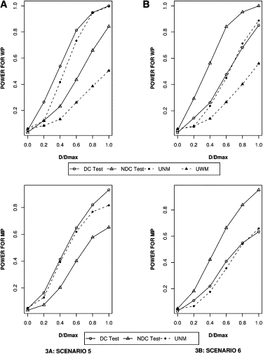
Power Comparison between XQTL and UNPHASED at a Single Marker

Data are 5000 replicate samples, each containing 250 families, with 2 offspring. X-linked QTL MAF is 0.2 and D_max = 0.16.

(A) Data simulated under scenario 5.

(B) Data simulated under scenario 6.

The upper two figures are for families with parental genotypes (WP), and lower two figures are for families with missing parental genotypes (MP). Solid lines with open circles show power of the XQTL DC test. Solid lines with open triangles show power of the XQTL NDC test. Dashed lines with closed circles show power of the UNPHASED quantitative haplotype test without sibsex modifier option (UNM). Dash lines with closed triangles show power of the UNPHASED quantitative haplotype test with sibsex modifier option (UWM), which cannot execute properly when both parents are missing.

Figure 4.

Power Comparison between XQTL and UNPHASED for Haplotypes of Two Loci

Data are 5000 replicate samples, each containing 250 families, with two offspring. The X-linked QTL MAF is 0.2, and the marker haplotype frequency distribution is {0.2, 0.3, 0.1, 0.4}. D_0max = 0.16, and D₁ = 0, and D₂ = 0. Figure 4A is for data simulated under scenario 5 and Figure 4B is for data simulated under scenario 6. Upper two figures are for families with parental genotypes (WP) and lower two figures are for families with missing parental genotype data (MP). Solid lines with open circles show power of XQTL DC test. Solid lines with open triangles show power of XQTL NDC test. Dash lines with closed circles show power of UNPHASED quantitative haplotype-test without sibsex modifier option (UNM). Dash lines with closed triangles show power of UNPHASED quantitative haplotype-test with sibsex modifier option (UWM), which cannot execute properly when both parents are missing.

XQTL Analysis for Age-at-Onset Data of PD and MAO Genes

XQTL tests were applied for analysis of nine MAOA SNP markers and six MAOB SNP markers.²⁸ SNP rs3027452, located in intron 5 of MAOB, shows strong evidence of association with AAO of PD (p = 0.037 in the DC test and p = 0.009 in the NDC test) at the 0.05 significance level. The estimate of the within-family coefficient (${\widehat{\mathit{\beta }}}_w$) is 7.21 in the DC test and 8.93 in the NDC test. We also studied the sex-specific genetic effects of MAOA and MAOB by dividing the full data into two single-sex subsets:^8,9 one set that had only males with the trait and another set that had only females with the trait. The genotypes of siblings without the trait, regardless of sex, were retained in both sets. The XQTL tests were applied separately on the two subsets with the use of parameters estimated in their respective sets. XQTL tests for SNP rs1799836, located in intron 13 of MAOB, show marginally significant association with AAO of PD in the female subset (p = 0.044 in the NDC test and p = 0.056 in the DC test).

XQTL haplotype tests for pairs of two markers in both MAOA and MAOB genes were not as promising as the single-locus association analysis. However, we found haplotypes of rs3027452 and rs1183035, located in intron 5 and the promoter region of MAOB, to have potential association to AAO, shown by global statistics in the NDC test (p = 0.037); this association was not shown in the DC test (p = 0.129). The haplotype-specific test results show that haplotype GC of SNPs rs3027452 and rs1183035 accounts for this association (p = 0.012) and meets the borderline of the Bonferroni-corrected significance level of 0.012. The sex-specific test results for SNPs rs3027452 and rs1183035 also show potential association between AAO and PD in the female subset (p = 0.019).

X-APL validation shows no strong association between rs3027452 and PD in overall data (p = 0.065) and EOPD data (p = 0.631), but there is a significant result in LOPD data (p = 0.022); also, there is no strong association between haplotypes of rs3027452–rs1183035 and PD in overall data (p = 0.134) and EOPD data (p = 0.853), but there is potential association in LOPD data (p = 0.034). In sex-specific subsets, we tested both single markers and haplotype markers with X-APL and replicated results only in the late-onset group in the female subset (p = 0.026 for SNP rs1799836 and p = 0.029 for haplotype rs3027452–rs1183035).

Discussion

We propose a family-based association method, XQTL, for testing association between X-linked marker alleles (or haplotypes) and a quantitative trait and for estimating the additive genetic value of a marker-allele (or haplotype). Our method has several attractive properties. First, the orthogonal decomposition controls spurious associations due to population stratification. Second, it can greatly increase power as compared with the existing software in the presence or absence of female X-inactivation. Third, family-based tests for association in regions with confirmed linkage might be subject to increased type I error rates. The use of variance-components analysis in which linkage is modeled as a random effect among related individuals avoids this problem.⁴ Finally, our method makes use of a mixed model that considers all of the effects from the major gene on the X chromosome, as well as the autosomal polygenic effect and the environmental factor.

Our simulations validate the type I error rates of XQTL tests when we vary the sample size, family structure, and marker-allele (or haplotype) frequencies. We show that XQTL is robust to a variety of biases, including the presence of linkage, population admixture, and a polygenic effect, although we note that a large polygenic variance (for example, ${\mathit{\sigma }}_{\mathit{g}}^2/V\ge 0.5$) or a very rare X-linked marker-allele (or haplotype) frequency (≤0.005) might cause inflated type I error. Missing parental information is common in late-onset diseases. We demonstrate that XQTL is valid when parental genotype data are unavailable.

We show the utility of XQTL applied to SNP data of MAOA and MAOB in a set of PD family data. Our analyses suggest that MAOB might play a role in increasing disease risk in the elderly and also influencing differential susceptibility between sexes.

The proposed method has limitations and is not optimal in all situations: (1) When parental genotypes are missing and the assumption of random mating is violated, the type I error rate of XQTL might be increased. (2) The global haplotype test provides accurate type I error rates for the common haplotypes but tends to be liberal for rare haplotypes. (3) The current version of XQTL handles haplotype analysis for only two SNP markers, but it is possible to extend to more than two markers under the same framework. However, increasing the number of markers will increase computational time. (4) One can apply the Bonferroni correction to address the mutliple testing of DC and NDC tests (α/2 = 0.025) at a single marker. However, because most X chromosome loci are subject to dosage compensation, in practice, one may obtain higher statistical power by applying the DC test even though the underlying appropriate QTL dosage model is unknown. Our simulations indicate that testing for association with an incorrect model is likely to result in a conservative test under the null hypothesis and a loss of power relative to the correct model under an alternative hypothesis. We therefore suggest that a sequential procedure be used: apply the DC test first, then apply the NDC test if the marker is not significant under the DC test. Because most loci are subject to dosage compensation, we suggest using significance levels of 0.04 for the DC test and 0.01 for the NDC test. On the basis of this testing strategy, the rs3027452 of MAOB remains interesting for the AAO trait in PD.

In conclusion, the XQTL method presented here is one of few family-based association methods for analyzing X-linked markers and quantitative traits. It is a powerful, robust, and efficient tool for evaluating association between single SNPs or haplotypes of two markers on the X chromosome and complex diseases. Accurate estimation of the effects for quantitative traits allows us to assess the relative degree to which traits are determined by X-linked genes. If it is preferable to estimate male and female major genetic variance separately, the variance-component model can be adjusted as suggested by Ekstrm.¹⁶ In addition, the XQTL method is also flexible for testing different null hypotheses. For instance, it is feasible to test ${\widehat{\mathit{\beta }}}_b={\widehat{\mathit{\beta }}}_w$ to evaluate evidence for population substructure and to test ${\mathit{\sigma }}_{\mathit{qf}}^2=0$ to distinguish X-linked QTL from other associated markers.²⁴ XQTL has been implemented in a software package and is available for several computer platforms. It is written in C and C++ and is distributed freely for public use.

Appendix A

EM Algorithm for Reconstructing Missing Parental Phased Genotypes

When parental genotype data are missing, we implement an EM algorithm²⁹ to reconstruct pseudo data and maximize the likelihood. The EM algorithm consists of an expectation (E) step and a maximization (M) step. The E step computes the expected value of the complete data likelihood, conditional on the observed genotypes of all family members and parental mating-type frequencies in the population. The M step updates parameters by maximizing the likelihood. The E and M steps iterate until the parameters converge.

Suppose that in a sample of N nuclear families, n_MF indicates the number of families that have female parent genotype (F) and male parent genotype (M). Because males are hemizygous for markers located on the X chromosome, haplotype phase is known if a male genotype is available. In females, however, there may be ambiguity when the marker is doubly heterozygous. With complete nuclear family data, the haplotype phase of the female can be deduced by tracing parent-offspring haplotype transmission. We denote C to be the genotypes of children in a family and use “.” notation to indicate missing parental genotypes or ambiguous phases. For example, n_M. denotes the number of families in which the mother's genotype or phase is unknown but the father's genotype is available. We define W as the weight for the phased genotype when there are missing or ambiguous data. Let E[(N_MF)^(t+1)] represent an expected count of parents with genotype (MF) at iteration t+1. Let Pr(MF)^(t) represent the parental mating-type frequencies in the population at iteration t.

The expected number of the parental mating follows:

$$E\left[N_{MF}^{(t+1)}\right]=n_{MF}\{\begin{array}{c}+\frac{{\prod }_{j\in \mathit{\zeta }}Pr\left(C_j\right|M,F)\times Pr{\left(MF\right)}^{\left(t\right)}}{{\sum }_{F_u}{\prod }_{j\in \mathit{\zeta }}Pr\left(C_j\right|M,F_u)\times Pr{\left(M{F}_u\right)}^{\left(t\right)}}\times n_{M\text{.}}\\ \\ +\frac{{\prod }_{j\in \mathit{\zeta }}Pr\left(C_j\right|M,F)\times Pr{\left(MF\right)}^{\left(t\right)}}{{\sum }_{M_u}{\prod }_{j\in \mathit{\zeta }}Pr\left(C_j\right|M_u,F)\times Pr{\left(M_{u}F\right)}^{\left(t\right)}}\times n_{\text{.}F}\\ \\ +\frac{{\prod }_{j\in \mathit{\zeta }}Pr\left(C_j\right|M,F)\times Pr{\left(MF\right)}^{\left(t\right)}}{{\sum }_{M_u{F}_u}{\prod }_{j\in \mathit{\zeta }}Pr\left(C_j\right|M_u,F_u)\times Pr{\left(M_u{F}_u\right)}^{\left(t\right)}}\times n_{\text{.}}\end{array}$$

in which ζ indicates the set of offspring in a family. M_u is all possible father genotypes within the family. F_u is all possible mother genotypes within the family. The corresponding component of the log-likelihood is given by E(N_MF) × log(Pr(MF|T)), in which Pr(MF|T) represents the parental mating-type frequencies conditional on the vector of observed offspring trait values.

The M step then maximizes the log likelihood to update parameter estimates.

$$Pr{\left(MF\right)}^{r+1}=\frac{E\left(N_{MF}^{(t+1)}\right)}{N}$$

in which N is total sample size. The EM algorithm cycles between the E and M steps until the parameters converge. Convergence is declared when the difference of the sum of squares between successive estimates is less than 1e − 12.

The phased genotypes are the weighted sum of possible phases, with weights proportional to the observed genotypes of all family members and estimations of parental mating-type frequencies in the population. Three scenarios are considered: (1) father's genotype is missing and mother's phase is known, (2) father's genotype is available and mother's genotype is missing, and (3) both parental genotypes are missing or father's genotype is missing and mother's phase is unknown.

$$W\left(F\right)=\{\begin{array}{c}\frac{{\prod }_{j\in \mathit{\zeta }}Pr\left(C_j\right|M,F)\times Pr\left(MF\right)}{{\sum }_{F_u}{\prod }_{j\in \mathit{\zeta }}Pr\left(C_j\right|M,F_u)\times Pr\left(M{F}_u\right)}\left(1\right)\\ \\ \frac{{\sum }_{M_u}{\prod }_{j\in \mathit{\zeta }}Pr\left(C_j\right|M_u,F)\times Pr\left(M_{u}F\right)}{{\sum }_{M_u}{\sum }_{F_u}{\prod }_{j\in \mathit{\zeta }}Pr\left(C_j\right|M_u,F_u)\times Pr\left(M_u{F}_u\right)}\left(3\right)\end{array}$$

$$W\left(M\right)=\{\begin{array}{c}\frac{{\prod }_{j\in \mathit{\zeta }}Pr\left(C_j\right|M,F)\times Pr\left(MF\right)}{{\sum }_{M_u}{\prod }_{j\in \mathit{\zeta }}Pr\left(C_j\right|M_u,F)\times Pr\left(M_{u}F\right)}\left(2\right)\\ \\ \frac{{\sum }_{F_u}{\prod }_{j\in \mathit{\zeta }}Pr\left(C_j\right|M,F_u)\times Pr\left(M{F}_u\right)}{{\sum }_{M_u}{\sum }_{F_u}{\prod }_{j\in \mathit{\zeta }}Pr\left(C_j\right|M_u,F_u)\times Pr\left(M_u{F}_u\right)}\left(3\right)\end{array}$$

The offspring genotype phases are determined by parental genotype phases.

Appendix B

β_wk with Allowance for Population Admixture at Two Tightly Linked Markers

We define μ_0i is the vector of population mean. R_k, k = 0,1,2,3, are the frequencies for haplotypes H₀ = A₁B₁, H₁ = A₁B₂, H₃ = A₂B₁, H₃ = A₂B₂ of the marker on the X chromosome. Assume that there is random mating of the population and random transmission of parental alleles to offspring and that the mean of the quantitative trait values of all samples is centered at 0, so that ${\mathit{\mu }}_0={\sum }_i{n}_i{\mathit{\mu }}_{0i}=0$. Let $M={\sum }_i{n}_i$, in which n_i is the number of offspring in the ith family. α₀, α₁, α₂ are the additive genetic values of X-linked marker haplotypes H₀, H₁, and H₂. We follow the Abecasis et al.¹³ procedures to prove the feasibility of the orthogonal model for the two-marker haplotype association test.

NDC Model

$$E\left(T\right)=\frac{{\Sigma }_i{n}_i{\mathit{\mu }}_{0i}}{M}+\frac{{\Sigma }_i{n}_{i}3(R_0{\mathit{\alpha }}_0+R_1{\mathit{\alpha }}_1+R_2{\mathit{\alpha }}_2)}{2M}=\frac{{\Sigma }_i{n}_{i}3(R_0{\mathit{\alpha }}_0+R_1{\mathit{\alpha }}_1+R_2{\mathit{\alpha }}_2)}{2M}$$

$$\begin{array}{c}E\left(g\right)=\frac{{\Sigma }_i{n}_i\left[{\Sigma }_0^{2}P(g=l|i)l\right]}{2M}+\frac{{\Sigma }_i{n}_i\left[{\Sigma }_0^{1}P(g=l|i)l\right]}{2M}\\ =\frac{{\Sigma }_i{n}_i}{2M}\left[\begin{array}{c}2R_0\\ 2R_1\\ 2R_2\end{array}\right]+\frac{{\Sigma }_i{n}_i}{2M}\left[\begin{array}{c}{R}_0\\ R_1\\ R_2\end{array}\right]=\frac{{\Sigma }_i{n}_i}{2M}\left[\begin{array}{c}3R_0\\ 3R_1\\ 3R_2\end{array}\right]\end{array}$$

$$\begin{array}{c}E\left(g^2\right)=\frac{{\Sigma }_i{n}_i\left[{\Sigma }_0^{2}P(g=l|i)l^2\right]}{2M}+\frac{{\Sigma }_i{n}_i\left[{\Sigma }_0^{1}P(g=l|i)l^2\right]}{2M}\\ =\frac{{\Sigma }_i{n}_i}{2M}\left[\begin{array}{c}2R_0^2+2R_0\\ 2R_1^2+2R_1\\ 2R_2^2+2R_2\end{array}\right]+\frac{{\Sigma }_i{n}_i}{2M}\left[\begin{array}{c}{R}_0\\ R_1\\ R_2\end{array}\right]=\frac{{\Sigma }_i{n}_i}{2M}\left[\begin{array}{c}2R_0^2+3R_0\\ 2R_1^2+3R_1\\ 2R_2^2+3R_2\end{array}\right]\end{array}$$

$$\begin{array}{c}E\left(gT\right)=\frac{{\Sigma }_i{n}_i\left[{\Sigma }_0^{2}P(g=l|i)l({\mathit{\mu }}_{0i}+l\mathit{\alpha })\right]}{2M}+\frac{{\Sigma }_i{n}_i\left[{\Sigma }_0^{2}P(g=l|i)l({\mathit{\mu }}_{0i}+l\mathit{\alpha })\right]}{2M}\\ =\frac{{\Sigma }_i{n}_i{\mathit{\mu }}_{0i}3(R_0+R_1+R_2)}{2M}+\frac{{\Sigma }_i{n}_i[(2R_0^2+3R_0){\mathit{\alpha }}_0+(2R_1^2+3R_1){\mathit{\alpha }}_1+(2R_2^2+3R_2){\mathit{\alpha }}_2]}{2M}\end{array}$$

$$E\left(b\right)=\frac{{\Sigma }_i{n}_i\sum P\left(\mathit{z}\right|i)E\left(b\right|z)}{M}=\frac{{\Sigma }_i{n}_i}{2M}\left[\begin{array}{c}3R_0\\ 3R_1\\ 3R_2\end{array}\right]=E\left(g\right)$$

$$E\left(b^2\right)=\frac{{\Sigma }_i{n}_i\sum P\left(z\right|i)E\left(b^2\right|z)}{M}=\frac{{\Sigma }_i{n}_i}{2M}\left[\begin{array}{c}3R_0^2+3R_0/2\\ 3R_1^2+3R_1/2\\ 3R_2^2+3R_2/2\end{array}\right]$$

$$E\left(bg\right)=\frac{{\Sigma }_i{n}_i\sum P\left(z\right|i)E\left(bg\right|z)}{M}=\frac{{\Sigma }_i{n}_i}{2M}\left[\begin{array}{c}3R_0^2+3R_0/2\\ 3R_1^2+3R_1/2\\ 3R_2^2+3R_2/2\end{array}\right]=E\left(b^2\right)$$

$$\begin{array}{c}E\left(bT\right)=\frac{{\Sigma }_i{n}_i\sum P\left(z\right|i)E\left(b{\mathit{\mu }}_{0i}\right|z)}{M}+\frac{{\Sigma }_i{n}_i\sum P\left(z\right|i)E\left(bg\mathit{\alpha }\right|z)}{M}\\ =\frac{{\Sigma }_i{n}_i{\mathit{\mu }}_{0i}3(R_0+R_1+R_2)}{2M}+\frac{{\Sigma }_i{n}_i[(3R_0^2+3R_0/2){\mathit{\alpha }}_0+(3R_1^2+3R_1/2){\mathit{\alpha }}_1+(3R_2^2+3R_2/2){\mathit{\alpha }}_2]}{2M}\end{array}$$

$$E\left(w\right)=E(g-b)=\left[\begin{array}{c}0\\ 0\\ 0\end{array}\right]$$

$$E\left(w^2\right)=E\left[{(g-b)}^2\right]=\frac{{\Sigma }_i{n}_i}{2M}\left[\begin{array}{c}-R_0^2+3R_0/2\\ -R_1^2+3R_1/2\\ -R_2^2+3R_2/2\end{array}\right]$$

$$E\left(wT\right)=E\left[(g-b)T\right]=\frac{{\Sigma }_i{n}_i[(-R_0^2+3R_0/2){\mathit{\alpha }}_0+(-R_1^2+3R_1/2){\mathit{\alpha }}_1+(-R_2^2+3R_2/2){\mathit{\alpha }}_2]}{2M}$$

$$V_w=E[w^2-E_w^2]=\frac{{\Sigma }_i{n}_i}{2M}\left[\begin{array}{c}-R_0^2+3R_0/2\\ -R_1^2+3R_1/2\\ -R_2^2+3R_2/2\end{array}\right]$$

$$C_{wT}=E_{wT}-E\left(w\right)E\left(T\right)=\frac{{\Sigma }_i{n}_i[(-R_0^2+3R_0/2){\mathit{\alpha }}_0+(-R_1^2+3R_1/2){\mathit{\alpha }}_1+(-R_2^2+3R_2/2){\mathit{\alpha }}_2]}{2M}$$

$${\widehat{\mathit{\beta }}}_w=\frac{C_{w,T}}{V_w}=\left[\begin{array}{c}{\mathit{\alpha }}_0\\ {\mathit{\alpha }}_1\\ {\mathit{\alpha }}_2\end{array}\right]$$

DC Model

$$E\left(T\right)=\frac{{\Sigma }_i{n}_i{\mathit{\mu }}_{0i}}{M}+\frac{{\Sigma }_i{n}_i(R_0{\mathit{\alpha }}_0+R_1{\mathit{\alpha }}_1+R_2{\mathit{\alpha }}_2)}{M}=\frac{{\Sigma }_i{n}_i(R_0{\mathit{\alpha }}_0+R_1{\mathit{\alpha }}_1+R_2{\mathit{\alpha }}_2)}{M}$$

$$E\left(g\right)=\frac{{\Sigma }_i{n}_i\left[{\Sigma }_0^{2}P(g=l|i)l\right]}{2M}+\frac{{\Sigma }_i{n}_i\left[{\Sigma }_0^{1}P(g=l|i)l\right]}{2M}=\frac{{\Sigma }_i{n}_i}{M}\left[\begin{array}{c}{R}_0\\ R_1\\ R_2\end{array}\right]$$

$$E\left(g^2\right)=\frac{{\Sigma }_i{n}_i\left[{\Sigma }_0^{2}P(g=l|i)l^2\right]}{2M}+\frac{{\Sigma }_i{n}_i\left[{\Sigma }_0^{1}P(g=l|i)l^2\right]}{2M}=\frac{{\Sigma }_i{n}_i}{2M}\left[\begin{array}{c}(R_0^2+3R_0)/2\\ (R_1^2+3R_1)/2\\ (R_2^2+3R_2)/2\end{array}\right]$$

$$\begin{array}{c}E\left(gT\right)=\frac{{\Sigma }_i{n}_i\left[{\Sigma }_0^{2}P(g=l|i)l({\mathit{\mu }}_{0i}+l\mathit{\alpha })\right]}{2M}+\frac{{\Sigma }_i{n}_i\left[{\Sigma }_0^{1}P(g=l|i)l({\mathit{\mu }}_{0i}+l\mathit{\alpha })\right]}{2M}\\ =\frac{{\Sigma }_i{n}_i{\mathit{\mu }}_{0i}(R_0+R_1+R_2)}{M}\\ +\frac{{\Sigma }_i{n}_i[(R_0^2+3R_0){\mathit{\alpha }}_0/2+(R_1^2+3R_1){\mathit{\alpha }}_1/2+(R_2^2+3R_2){\mathit{\alpha }}_2/2]}{2M}\end{array}$$

$$E\left(b\right)=\frac{{\Sigma }_i{n}_i\sum P\left(z\right|i)E\left(b\right|z)}{M}=\frac{{\Sigma }_i{n}_i}{M}\left[\begin{array}{c}{R}_0\\ R_1\\ R_2\end{array}\right]=E\left(g\right)$$

$$E\left(b^2\right)=\frac{{\Sigma }_i{n}_i\sum P\left(z\right|i)E\left(b^2\right|z)}{M}=\frac{{\Sigma }_i{n}_i}{M}\left[\begin{array}{c}5R_0^2/8+3R_0/8\\ 5R_1^2/8+3R_1/8\\ 5R_2^2/8+3R_2/8\end{array}\right]$$

$$\begin{array}{c}E\left(bg\right)=\frac{{\Sigma }_i{n}_i\sum P\left(z\right|i)E\left(bg\right|z)}{M}\\ =\frac{{\Sigma }_i{n}_i}{M}\left[\begin{array}{c}11R_0^2/16+5R_0/16\\ 11R_1^2/16+5R_1/16\\ 11R_2^2/16+5R_2/16\end{array}\right]\end{array}$$

$$\begin{array}{c}E\left(bT\right)=\frac{{\Sigma }_i{n}_i\sum P\left(z\right|i)E\left(b{\mathit{\mu }}_{0i}\right|z)}{M}+\frac{{\Sigma }_i{n}_i\sum P\left(z\right|i)E\left(bg\mathit{\alpha }\right|z)}{M}\\ =\frac{{\Sigma }_i{n}_i{\mathit{\mu }}_{0i}(R_0+R_1+R_2)}{M}\\ +\frac{{\Sigma }_i{n}_i[(11R_0^2+5R_0){\mathit{\alpha }}_0/16+(11R_1^2+5R_1){\mathit{\alpha }}_1/16+(11R_2^2+5R_2){\mathit{\alpha }}_2/16]}{M}\end{array}$$

$$E\left(w\right)=E(g-b)=\left[\begin{array}{c}0\\ 0\\ 0\end{array}\right]$$

$$E\left(w^2\right)=E\left[{(g-b)}^2\right]=\frac{{\Sigma }_i{n}_i}{2M}\left[\begin{array}{c}-R_0^2+R_0\\ -R_1^2+R_1\\ -R_2^2+R_2\end{array}\right]$$

$$E\left(wT\right)=E\left[(g-b)T\right]=\frac{{\Sigma }_i{n}_i[(-7R_0^2+7R_0){\mathit{\alpha }}_0+(-7R_1^2+7R_1){\mathit{\alpha }}_1+(-7R_2^2+7R_2){\mathit{\alpha }}_2]}{16M}$$

$$V_w=E[w^2-E_w^2]=\frac{{\Sigma }_i{n}_i}{2M}\left[\begin{array}{c}-R_0^2+R_0\\ -R_1^2+R_1\\ -R_2^2+R_2\end{array}\right]$$

$$C_{wT}=E_{wT}-E\left(w\right)E\left(T\right)=\frac{{\Sigma }_i{n}_i[(-7R_0^2+7R_0){\mathit{\alpha }}_0+(-7R_1^2+7R_1){\mathit{\alpha }}_1+(-7R_2^2+7R_2){\mathit{\alpha }}_2]}{16M}$$

$${\widehat{\mathit{\beta }}}_w=\frac{C_{w,T}}{V_w}=\left[\begin{array}{c}7{\mathit{\alpha }}_0/8\\ 7{\mathit{\alpha }}_1/8\\ 7{\mathit{\alpha }}_2/8\end{array}\right]$$

Appendix C

REML is an appropriate maximum likelihood method for a multivariate normal distribution, accounting for the loss of degrees of freedom due to fitting fixed effects. First, we discuss the first derivatives of the likelihood function from REML. T is the vector including observed offspring trait values. The matrix of fixed effects is X = [$\tilde{1}$, ${\tilde{b}}_i$, ${\tilde{w}}_{ij}$]. The vector of regression coefficient is β = [μ₀, β_b, β_w]. The vector of variance components is σ² = [${\mathit{\sigma }}_{\mathit{qm}}^2$, ${\mathit{\sigma }}_{\mathit{g}}^2$, ${\mathit{\sigma }}_{\mathit{e}}^2$].

$$\frac{\mathit{\partial }LogL}{\mathit{\partial }\mathit{\beta }}=X\prime \Omega (T-X\mathit{\beta })$$

$$\frac{\mathit{\partial }\Omega }{\mathit{\partial }{\mathit{\sigma }}_l^2}=V_l=\{\begin{array}{c}\Pi (l=qm)\\ 2\Phi (l=g)\\ I(l=e)\end{array}$$

Given KX = 0 and P = K′(KΩK′)^-1K,

$$\begin{array}{c}P=K\prime {(K\Omega K\prime )}^{-1}K\\ \frac{\mathit{\partial }LogL}{\mathit{\partial }{\mathit{\sigma }}_l^2}=-\frac{1}{2}tr\left({\Omega }^{-1}{V}_l\right)+\frac{1}{2}(T-X\widehat{\mathit{\beta }})\prime {\Omega }^{-1}{V}_l{\Omega }^{-1}(T-X\widehat{\mathit{\beta }})\\ =-\frac{1}{2}tr\left(P{V}_l\right)+\frac{1}{2}T\prime P{V}_{l}PT\end{array}$$

(see Searle et al.³⁰). We use SOLAR¹⁴ to estimate IBD probability matrix Π.

In Fisher's scoring method,

$$F=-E\left(\frac{{\mathit{\partial }}^{2}LogL}{\mathit{\partial }{\mathit{\sigma }}_l^2\mathit{\partial }{\mathit{\sigma }}_m^2}\right)=\frac{1}{2}\left[\begin{array}{c}tr(P\Pi P\Pi )tr(P\Pi P2\Phi )tr(P\Pi PI)\\ tr(P\Pi P2\Phi )tr(P2\Phi P2\Phi )tr(P2\Phi PI)\\ tr(P\Pi PI)tr(P2\Phi PI)tr\left(PIPI\right)\end{array}\right]$$

At t+1 iteration,

$${\mathit{\sigma }}_l^{2^{(t+1)}}={\mathit{\sigma }}_l^{2\left(t\right)}+{\left(F^{\left(t\right)}\right)}^{-1}\frac{\mathit{\partial }LogL}{\mathit{\partial }{\mathit{\sigma }}_l^2}{|}_{{\mathit{\sigma }}_l^2={\mathit{\sigma }}_l^{2\left(t\right)}}$$

General Least-Squares Equation estimates the fixed effects:

$$\begin{array}{c}(X\prime {\Omega }^{-1}X)\mathit{\beta }=X\prime {\Omega }^{-1}T\\ {\widehat{\mathit{\beta }}}^{(t+1)}={[X\prime {\left({\Omega }^{(t+1)}\right)}^{-1}X]}^{-1}X\prime {\left({\Omega }^{(t+1)}\right)}^{-1}T\end{array}$$

The variance components and the fixed effects are updated at each iteration and then plugged into the likelihood. We applied a step-halving algorithm²⁵ to control convergence whenever a variance-component estimate approached zero. Convergence is declared when the difference of the sum of squares between successive estimates is less than 1e − 12.

Web Resources

The URLs for data presented herein are as follows:

• Online Mendelian Inheritance in Man (OMIM), http://www.ncbi.nlm.nih.gov/omim/

• UNPHASED 3.0.8, http://www.mrc-bsu.cam.ac.uk/personal/frank/software/unphased/

• X-APL, http://www.mihg.org/weblog/about_us/2008/09/software-download.html

• XQTL, http://wwwchg.duhs.duke.edu/research/software.html and http://www.mihg.org

References

- 1.Spielman R.S., McGinnis R.E., Ewens W.J. Transmission test for linkage disequilibrium: The insulin gene region and insulin-dependent diabetes mellitus (IDDM) Am. J. Hum. Genet. 1993;52:506–516. [PMC free article] [PubMed] [Google Scholar]
- 2.Weinberg C.R., Wilcox A.J., Lie R.T. A log-linear approach to case- parent-triad data: Assessing effects of disease genes that act either directly or through maternal effects and that may be subject to parental imprinting. Am. J. Hum. Genet. 1998;62:969–978. doi: 10.1086/301802. [DOI] [PMC free article] [PubMed] [Google Scholar]
- 3.Allison D.B. Transmission-disequilibrium tests for quantitative traits. Am. J. Hum. Genet. 1997;60:676–690. [PMC free article] [PubMed] [Google Scholar]
- 4.Abecasis G.R., Cardon L.R., Cookson W.O. A general test of association for quantitative traits in nuclear families. Am. J. Hum. Genet. 2000;66:279–292. doi: 10.1086/302698. [DOI] [PMC free article] [PubMed] [Google Scholar]
- 5.Liu J., Nyholt D.R., Magnussen P., Parano E., Pavone P., Geschwind D., Lord C., Iversen P., Hoh J., Ott J. A genomewide screen for autism susceptibility loci. Am. J. Hum. Genet. 2001;69:327–340. doi: 10.1086/321980. [DOI] [PMC free article] [PubMed] [Google Scholar]
- 6.Ohman M., Oksanen L., Kaprio J., Koskenvuo M., Mustajoki P., Rissanen A., Salmi J., Kontula K., Peltonen L. Genome-wide scan of obesity in finnish sibpairs reveals linkage to chromosome Xq24. J. Clin. Endocrinol. Metab. 2000;85:3183–3190. doi: 10.1210/jcem.85.9.6797. [DOI] [PubMed] [Google Scholar]
- 7.Pankratz N., Nichols W.C., Uniacke S.K., Halter C., Murrell J., Rudolph A., Shults C.W., Conneally P.M., Foroud T., Group P.S. Genome-wide linkage analysis and evidence of gene-by-gene interactions in a sample of 362 multiplex Parkinson disease families. Hum. Mol. Genet. 2003;12:2599–2608. doi: 10.1093/hmg/ddg270. [DOI] [PubMed] [Google Scholar]
- 8.Zhang L., Martin E.R., Chung R.-H., Li Y.-J., Morris R.W. X-LRT: A likelihood approach to estimate genetic risks and test association with X-linked markers using a case-parents design. Genet. Epidemiol. 2008;32:370–380. doi: 10.1002/gepi.20311. [DOI] [PubMed] [Google Scholar]
- 9.Chung R.-H., Morris R.W., Zhang L., Li Y.-J., Martin E.R. X-APL: An improved family-based test of association in the presence of linkage for the X chromosome. Am. J. Hum. Genet. 2007;80:59–68. doi: 10.1086/510630. [DOI] [PMC free article] [PubMed] [Google Scholar]
- 10.Ding J., Lin S., Liu Y. Monte Carlo pedigree disequilibrium test for markers on the X chromosome. Am. J. Hum. Genet. 2006;79:567–573. doi: 10.1086/507609. [DOI] [PMC free article] [PubMed] [Google Scholar]
- 11.Horvath S., Laird N.M., Knapp M. The transmission/disequilibrium test and parental-genotype reconstruction for X-chromosomal markers. Am. J. Hum. Genet. 2000;66:1161–1167. doi: 10.1086/302823. [DOI] [PMC free article] [PubMed] [Google Scholar]
- 12.Wiener H., Elston R.C., Tiwari H.K. X-linked extension of the revised Haseman-Elston algorithm for linkage analysis in sib pairs. Hum. Hered. 2003;55:97–107. doi: 10.1159/000072314. [DOI] [PubMed] [Google Scholar]
- 13.Abecasis G.R., Cherny S.S., Cookson W.O., Cardon L.R. Merlin–rapid analysis of dense genetic maps using sparse gene flow trees. Nat. Genet. 2002;30:97–101. doi: 10.1038/ng786. [DOI] [PubMed] [Google Scholar]
- 14.Almasy L., Blangero J. Multipoint quantitative-trait linkage analysis in general pedigrees. Am. J. Hum. Genet. 1998;62:1198–1211. doi: 10.1086/301844. [DOI] [PMC free article] [PubMed] [Google Scholar]
- 15.Lange K., Sobel E. Variance component models for X-linked QTLs. Genet. Epidemiol. 2006;30:380–383. doi: 10.1002/gepi.20158. [DOI] [PubMed] [Google Scholar]
- 16.Ekstrøm C.T. Multipoint linkage analysis of quantitative traits on sex-chromosomes. Genet. Epidemiol. 2004;26:218–230. doi: 10.1002/gepi.10310. [DOI] [PubMed] [Google Scholar]
- 17.Fulker D.W., Cherny S.S., Cardon L.R. Multipoint interval mapping of quantitative trait loci, using sib pairs. Am. J. Hum. Genet. 1995;56:1224–1233. [PMC free article] [PubMed] [Google Scholar]
- 18.Kruglyak L., Lander E.S. Complete multipoint sib-pair analysis of qualitative and quantitative traits. Am. J. Hum. Genet. 1995;57:439–454. [PMC free article] [PubMed] [Google Scholar]
- 19.Kent J.W., Dyer T.D., Blangero J. Estimating the additive genetic effect of the X chromosome. Genet. Epidemiol. 2005;29:377–388. doi: 10.1002/gepi.20093. [DOI] [PMC free article] [PubMed] [Google Scholar]
- 20.Bulmer M. Oxford University Press; New York: 1985. The Mathematical Theory of Quantitative Genetics. [Google Scholar]
- 21.Dudbridge F. Likelihood-based association analysis for nuclear families and unrelated subjects with missing genotype data. Hum. Hered. 2008;66:87–98. doi: 10.1159/000119108. [DOI] [PMC free article] [PubMed] [Google Scholar]
- 22.Falconer D.S. Longman Scientific & Technical; London: 1989. Introduction to Quantitative Genetics. [Google Scholar]
- 23.Fulker D.W., Cherny S.S., Sham P.C., Hewitt J.K. Combined linkage and association sib-pair analysis for quantitative traits. Am. J. Hum. Genet. 1999;64:259–267. doi: 10.1086/302193. [DOI] [PMC free article] [PubMed] [Google Scholar]
- 24.Cardon L.R., Abecasis G.R. Some properties of a variance components model for fine-mapping quantitative trait loci. Behav. Genet. 2000;30:235–243. doi: 10.1023/a:1001970425822. [DOI] [PubMed] [Google Scholar]
- 25.Jennrich J., PF S. Newton-Raphson and related algorithms for maximum likelihood variance component estimation. Technometrics. 1976;18:11–17. [Google Scholar]
- 26.Falconer D.S., Mackay T.F. Introduction to Quantitative Genetics. In: Cummings Benjamin., editor. 4th edition. Addison Wesley Longman; Essex, UK: 1996. [Google Scholar]
- 27.Li Y.-J., Scott W.K., Hedges D.J., Zhang F., Gaskell P.C., Nance M.A., Watts R.L., Hubble J.P., Koller W.C., Pahwa R. Age at onset in two common neurodegenerative diseases is genetically controlled. Am. J. Hum. Genet. 2002;70:985–993. doi: 10.1086/339815. [DOI] [PMC free article] [PubMed] [Google Scholar]
- 28.Kang S.J., Scott W.K., Li Y.-J., Hauser M.A., van der Walt J.M., Fujiwara K., Mayhew G.M., West S.G., Vance J.M., Martin E.R. Family-based case-control study of MAOA and MAOB polymorphisms in Parkinson disease. Mov. Disord. 2006;21:2175–2180. doi: 10.1002/mds.21151. [DOI] [PubMed] [Google Scholar]
- 29.Dempster A., Laird N., Rubin D. Maximum likelihood from incomplete data via the EM algorithm. J. R. Stat. Soc. [Ser A] 1977;39:1–38. [Google Scholar]
- 30.Searle S., Casella G., McCulloch C. John Wiley and Sons; New York: 1992. Variance Components. [Google Scholar]