Improved classifier for computer-aided polyp detection in CT Colonography by nonlinear dimensionality reduction

Abstract

Computer-aided detection (CAD) has been shown to be feasible for polyp detection on computed tomography (CT) scans. After initial detection, the dataset of colonic polyp candidates has large-scale and high dimensional characteristics. In this article, we propose a nonlinear dimensionality reduction method based on diffusion map and locally linear embedding (DMLLE) for large-scale datasets. By selecting partial data as landmarks, we first map these points into a low dimensional embedding space using the diffusion map. The embedded landmarks can be viewed as a skeleton of whole data in the low dimensional space. Then by using the locally linear embedding algorithm, nonlandmark samples are mapped into the same low dimensional space according to their nearest landmark samples. The local geometry is preserved in both the original high dimensional space and the embedding space. In addition, DMLLE provides a faithful representation of the original high dimensional data at coarse and fine scales. Thus, it can capture the intrinsic distance relationship between samples and reduce the influence of noisy features, two aspects that are crucial to achieving high classifier performance. We applied the proposed DMLLE method to a colonic polyp dataset of 175 269 polyp candidates with 155 features. Visual inspection shows that true polyps with similar shapes are mapped to close vicinity in the low dimensional space. We compared the performance of a support vector machine (SVM) classifier in the low dimensional embedding space with that in the original high dimensional space, SVM with principal component analysis dimensionality reduction and SVM committee using feature selection technology. Free-response receiver operating characteristic analysis shows that by using our DMLLE dimensionality reduction method, SVM achieves higher sensitivity with a lower false positive rate compared with other methods. For $6–9\mathrm{mm}$ polyps (193 true polyps contained in test set), when the number of false positives per patient is 9, SVM with DMLLE improves the average sensitivity from 70% to 83% compared with that of an SVM committee classifier which is a state-of-the-art method for colonic polyp detection $(p<0.001)$.

INTRODUCTION

Colon cancer is the second leading cause of cancer-related deaths in the United States. Optical colonoscopy (OC) is a traditional and effective method for colonic polyp detection. However, OC is invasive and requires the sedation of patients to reduce discomfort. Computed tomographic colonography (CTC), also known as virtual colonoscopy (VC), is an imaging technique based on x-ray penetration and is less invasive than optical colonoscopy. When CTC is performed in conjunction with computer-aided detection (CAD) software, the screening becomes easier on the patient, less time-consuming, and more accurate for the radiologist.^{1, 2, 3}

CAD systems to detect polyps using CTC have been under investigation in the past decades. Most of these systems used features computed from the original CT dataset, such as surface curvature,⁴ volumetric cluster,⁵ edge displacement fields,⁶ surface patch,⁷ deformable models,⁸ surface normal overlap,⁹ and wavelet texture features from 2D endoluminal projection images,¹⁰ etc.

Shape analysis plays an important role in the detection of colonic polyps. Colonic polyps appear as bulbous protrusions that adhere to the inner wall of the colon or on the folds, which have elongated, ridgelike structures. It is possible to extract more than 150 features from each polyp candidate. However, the high dimension (number of features) is an obstacle to the processing of the data. For example, it will bring us a lot of trouble when we approximate functions or estimate the density of data in high dimensional space. It is called the curse of dimensionality. For colonic polyp detection problem, high dimensionality will make it hard to learn a good decision boundary or function in the space where the data reside. Especially when the data are noisy, high dimensions may cause highly biased estimates of the distance relationship of samples, and thereby reduce the accuracy of predictions. Thus, a point of interest is finding a compact representation of polyp candidates in a low dimensional space. Classical techniques for dimensionality reduction, such as principal components analysis (PCA) are designed for data whose submanifold is embedded linearly or almost linearly in the observation space.¹¹ Because many data from real applications, such as visual perception,¹² have nonlinear submanifold structures, there has been a surge in the research of nonlinear dimensionality reduction (NLDR) in recent years. The representative methods of NLDR include the local approaches locally linear embedding (LLE),¹³ Laplacian eigenmaps¹⁴ and global approaches (ISOMAP),¹² diffusion map,^{15, 16, 17} etc. In these nonlinear methods, local methods try to preserve the local geometry of the data in low dimensional space; global approaches tend to give a more faithful representation of the data’s global structure.

Here we attempt to explore, by dimensional reduction, the extraction of useful information from polyp candidates. Learning and testing are performed in a low dimensional space, and thus the classifier can be more effectively trained, as compared with that in the original high dimensional space. The outline of the article is as follows: In Sec. 2 we introduce the pipeline of our CAD system. Section 3 proposes a nonlinear dimensionality reduction method called diffusion map locally linear embedding (DMLLE) for large-scale datasets. We also discuss the relationship between DMLLE and Nyström extension^{18, 19, 20} in this section. Section 4 shows the experimental results and analysis of DMLLE on a large-scale colonic polyp dataset. Finally, Sec. 5 concludes with a short summary.

CAD PIPELINE

Our CTC CAD protocol consists of four main parts. First, when the CAD software reads a CT scan, it automatically identifies the colon wall and lumen based on a region growing and isosurface technique.⁴ This step is called colon segmentation. Secondly, for each point on the colon surface, geometric and local volumetric properties are analyzed and filtered. The specifications for the filter are elliptical curvature of the peak subtype, mean curvature range $-2.5\text{to}-0.7{\mathrm{cm}}^{-1}$, $⩾8$ vertices, $⩾0.25\mathrm{cm}$ diameter, and sphericity $⩽1.2$. The filtered surface vertices are then clustered based on connectivity. The centroid of each cluster is used as a polyp candidate.⁴ The candidates are then passed to a segmentor, where the detection boundaries are delineated. The segmentation is based on a combination of knowledge-guided intensity adjustment, fuzzy clustering, and adaptive deformable model.⁸ The third step is feature extraction, where characteristic features, such as shape and texture, are calculated from the segmented detection and its surrounding regions. Finally, the fourth provision step is discrimination, whereby the extracted features are subjected to learning algorithms.²¹ These algorithms are applied to sets of training data with known labels of each polyp candidate. The learned classifier then predicts the label of each new polyp candidate. Experienced operators manually traced the boundaries of all polyps in our database and used them as the reference standard in our training and validation process.

A LARGE-SCALE DIMENSIONALITY REDUCTION METHOD BASED ON DIFFUSION MAP AND LLE

To apply the dimensionality reduction method in the CAD system and make it practical, two major problems need to be considered. The first one is the large-scale problem. Our dataset contains CT scans of more than 1200 patients. After preprocessing, we get more than 170 000 polyp candidates altogether. How to deal with such a large-scale dataset is a big challenge for current dimensionality reduction methods. The second one is the noise problem. For the complex environment inside the colon and the artifacts induced by segmentation, the features extracted from a polyp candidate contain much noise. In addition, for clinical application, we focus on the detection of small polyps whose size is in the range of $6\text{to}9\mathrm{mm}$. Because the resolution of 3D CT images is limited, the features of small polyp candidates are not as accurate as that of bigger polyp candidates. So we should consider the noise resistance ability of dimension reduction methods. For example, if two submanifolds are linked by noisy samples in original high dimension space, then the performance of the ISOMAP algorithm¹² will drop because the geodesic distances between samples distributed on these two submanifolds will be close. The same is true for the LLE method.¹³

Construct global skeleton in low dimensional space by using diffusion map

R. R. Coifman et al. proposed a unified framework for dimensionality reduction, graph partitioning, and dataset parametrization based on the Markov random walk on the data.^{15, 16, 17} The method called diffusion map is noise resistant because the calculation of distance between two samples considers all paths between them. So noisy samples will have little influence on the calculation of similarities between samples.

Assume that a system contains n samples $X=\{x_1,x_2,\dots ,x_n\}$. The weight function $w(x,y)$ depicts the distance relationship between samples x and y. The transition probability of going from node x to y in one step is $p_1(x,y)=w(x,y)∕d\left(x\right)$, where $d\left(x\right)={\sum }_{z∊X}w(x,z)$ is called the degree of node x. The one step Markov transition matrix P has a set of right eigenvectors corresponding eigenvalues $1=\mid {\lambda }_0\mid ⩾\mid {\lambda }_1\mid ⩾\dots ⩾\mid {\lambda }_{n-1}\mid :P{\psi }_j={\lambda }_j{\psi }_j$. The diffusion map is defined as

$${\Psi }_t:x\mapsto ({\lambda }_1^t{\psi }_1\left(x\right),{\lambda }_2^t{\psi }_2\left(x\right),\dots ,{\lambda }_{q\left(t\right)}^t{\psi }_{q\left(t\right)}\left(x\right)),$$

where t represents the steps of Markov random walk on the graph and $q\left(t\right)$ is the number of dimensions of embedding space.

In the diffusion map algorithm,¹⁷ we need to solve an eigenvalue decomposition problem in which the size of the Markov probability transition matrix is $n\times n$. For real large-scale application, it would be prohibitive to do the eigenvalue decomposition task. For example, if an application has 100 000 samples, then the Markov probability transition matrix will need about $80\mathrm{gigabytes}$ of memory space. The eigenvalue decomposition cannot be done in acceptable time by using current mainstream PC servers. So how to extend the Diffusion Map algorithm and make it applicable for large-scale data are critical for some real applications.

Inspired by the idea of landmarks in the ISOMAP algorithm,¹² here we consider just randomly selecting partial data and embedding them into a lower dimensional space by using Diffusion Map. These selected samples are viewed as landmarks. The number of landmarks is chosen according to the capability of eigenvalue decomposition of our computation resource. As we know, Diffusion Map uses multistep Markov transition probability as the measure of distance between any two points. So it can preserve the global geometry structure of the original dataset in low dimensional space and be viewed as a global dimension reduction method. By using Diffusion Map just for these landmarks, we can construct a global skeleton of the whole data in the low dimensional space.

Embed nonlandmark samples by using Locally Linear Embedding

With the skeleton in low dimension, now the problem is how to embed other samples (nonlandmarks) into the same low dimensional space. As we mentioned before, local dimension reduction methods try to keep the local distance relationship of data in embedded space. LLE is such a typical algorithm.¹³ The LLE algorithm contains three steps:

• (1)Step 1 (discovering neighbors). For each $x_i$, find the K nearest neighbors in the original high dimensional dataset.
• (2)Step 2 (constructing the approximation matrix). Compute the weights $W_{ij}$ that best reconstruct $x_i$ from its nearest neighbors. $W_{ij}$ should minimize the following reconstruction error: ${\sum }_{i=1}^n\Vert x_i-{\sum }_{j=1}^K{W}_{ij}{x}_{i_j}\Vert$ with the constraints ${\sum }_j{W}_{ij}=1$ for each i.
• (3)Step 3 (embedding to low dimensional space). Compute the embedding by choosing ${\psi }_i$, which minimizes ${\sum }_{i=1}^n\Vert {\psi }_i-{\sum }_{j=1}^K{W}_{ij}{\psi }_{i_j}\Vert$ where ${\psi }_{i_j},j=1,\dots ,K$ are embeddings of the K nearest neighbors of sample i in the low dimensional space.

Many proposed dimensionality reduction methods are related to eigenvalue decomposition problems. The Nyström method provides a way to connect the eigenvalue decomposition problem with eigenfunction problems, which can be used to embed out-of-sample examples.^{18, 19, 20} Given a Hilbert space $H_p$ of functions, consider the following eigenfunction problems: ${\int }_0^{1}K(x,y)\varphi \left(y\right)dy=\lambda \varphi \left(x\right)$. By using training samples $x_i$, $i=1,2,\dots ,n$, we can approximate this integral as $1∕n{\sum }_{j=1}^{n}K(x,x_j)\widehat{\varphi }\left(x_j\right)$, where $\widehat{\varphi }\left(x\right)$ is an approximation to the true eigenfunction $\varphi \left(x\right)$. Assuming ${\lambda }_1,{\lambda }_2,\dots ,{\lambda }_n$ and ${\psi }_1,{\psi }_2,\dots ,{\psi }_n$ are eigenvalues and corresponding eigenvectors of the kernel matrix K of samples $x_i$, $i=1,2,\dots ,n$. The Nyström extension for each eigenfunction ${\widehat{\varphi }}_i$ is defined as: ${\widehat{\varphi }}_i\left(x\right)=1∕n{\lambda }_i{\sum }_{j=1}^{n}K(x,x_j){\psi }_i\left(x_j\right)$. Based on the Nyström extension, for dimension reduction problems we can embed a new sample into the low dimensional space by using a kernel function K and calculated eigenvectors ${\psi }_1,{\psi }_2,\dots ,{\psi }_n$. So Nyström extension provides another way to embed nonlandmark samples to the low dimensional space. We call it the DM Nyström method.¹⁹

Then, what is the relationship between LLE and the Nyström extension? It seems that LLE is a local interpolation method and the Nyström extension is a global interpolation method for inference embedding of a newcoming sample based on eigenvectors calculated from training samples. As pointed by Y. Bengio et al.,²⁰ by introducing an extra parameter μ and defining the kernel matrix as ${\tilde{K}}_{\mu }=(\mu -1){\delta }_{ij}+W_{ij}+W_{ji}-{\sum }_k{W}_{ki}{W}_{kj}$, the embedding for a new sample x in LLE algorithm also follows Nyström extension mechanism in essence. It can be viewed as a variation of the basic Nyström extension.

Borrowed from the idea of LLE, by using the embeddings of landmarks, we can embed nonlandmarks to the low dimensional space and maintain the local geometry relationship at the same time. Each nonlandmark sample in embedding space is constructed by using K nearest landmark embeddings. The locally linear weight matrix W is computed in the original high dimensional space.

Framework of DMLLE algorithm

Based on the previous introduction, the framework of the proposed large-scale dimensionality reduction method is as follows. Because it is based on the diffusion map algorithm and LLE, we call it the diffusion map locally linear embedding algorithm.

• (1)Step 1. Randomly select partial samples as landmarks from whole data and calculate the Markov probability transition matrix of them.
• (2)Step 2. Do eigenvalue decomposition and construct the low dimensional embeddings of the landmarks by using diffusion map.
• (3)Step 3. Compute the weights $W_{ij}$ that best reconstruct nonlandmark point $x_i$ from its nearest landmarks in original high dimensional space. $W_{ij}$ should minimize the following reconstruction error: ${\sum }_{i=1}^n\Vert x_i-{\sum }_{j=1}^K{W}_{ij}{x}_{i_j}\Vert$ with the constraints ${\sum }_j{W}_{ij}=1$ for each i.
• (4)Step 4. Compute the low dimensional embedding of nonlandmark point $x_i$ by choosing ${\psi }_i$, which minimizes ${\sum }_{i=1}^n\Vert {\psi }_i-{\sum }_{j=1}^K{W}_{ij}{\psi }_{i_j}\Vert$, where j is among the K-nearest landmarks of i.

By using dimension reduction, we hope we can capture the intrinsic distance relationship of samples located on low dimensional manifold. That would be very helpful for the subsequent supervised learning task. To evaluate the effectiveness of our method for the detection of colonic polyps, we compared the performance of the support vector machine (SVM)²² using DMLLE with that of SVM using the PCA dimension reduction method and SVM using all features. In addition, recent research shows that feature selection provides another feasible way to select the most informative features from the colonic polyp dataset.^{21, 23} So we also compared the performance of SVM after DMLLE dimension reduction with that of an SVM committee in which the features used by each SVM classifier are a subset of whole features from feature selection.²¹ In the next section, we will show the comparison results.

EXPERIMENTS

CT Colonography Data

To evaluate our method, we applied DMLLE to a CT colonography dataset that contains the CT scans of 1186 patients. Every patient was scanned twice—once supine and once prone. Each scan was done during a single breath hold using a four-channel or eight-channel CT scanner (General Electric LightSpeed or LightSpeed Ultra, GE Healthcare Technologies, Waukesha, WI). CT scanning parameters included $1.25\text{to}2.5\mathrm{mm}$ section collimation, $15\mathrm{mm}∕\mathrm{s}$ table speed a $1\mathrm{mm}$ reconstruction interval, $100\mathrm{mA}\mathrm{s}$, and $120\mathrm{kVp}$. These scans were divided into a training set (containing 395 patients) and a test set (containing 791 patients). After 3D colon surface segmentation and polyp candidate segmentation, we extracted 155 features from each polyp candidate. These features were calculated from a polyp candidate based on its shape, volume, etc. Most features were especially related with various curvatures of a polyp candidate. For the training set, we got 58 406 polyp candidates that included 85 true polyp detections (coming from 54 physical polyps) whose sizes ranged from $6\text{to}9\mathrm{mm}$ and 52 true polyp detections (coming from 25 physical polyps) whose sizes were greater than $9\mathrm{mm}$. The test set contained 116 863 polyp candidates in which there were 193 $6–9\mathrm{mm}$ true polyp detections (coming from 123 physical polyps) and 87 true polyp detections (coming from 44 physical polyps), which are bigger than $9\mathrm{mm}$. To focus on the detection performance of our method, here we did not consider uniqueness, meaning that several true polyp candidates may have come from the same physical polyp. Since current detection algorithms perform very well on true polyps that are greater than $9\mathrm{mm}$,³ we focused on the detection of true polyps whose sizes ranged from $6\text{to}9\mathrm{mm}$. These polyps are important because the earlier we can find a polyp in its growth stage, the higher the probability we may prevent its developing into a malignant tumor.

Experimental results

After deleting those true polyps that are greater than $9\mathrm{mm}$ or less than $6\mathrm{mm}$, we got 58 336 polyp candidates from the training set and 116 740 polyp candidates from the test set. We randomly selected 1000 candidates from them as landmarks. Because true polyps are very few compared with false polyps, here we selected all true polyps as landmarks. A radial basis function (RBF) kernel with a width of $1∕155$ was used to capture the distance relationship between landmarks. The Markov probability transition matrix was generated according to the kernel matrix. The step of Markov transition is 1. The previous parameters were selected according to the cross validation on the training set. After diffusion map, we reduced the dimensions of the original data to 30 dimensions. Figure 1 shows the distribution of eigenvalues of Markov matrix from the second largest eigenvalue to the 30th eigenvalue (the largest eigenvalue of Markov matrix is always 1). The eigenvalues drop quickly and there is an elbow point around the 30th eigenvalue. Because the approximation quality of diffusion map is controlled by the distribution of eigenvectors,^{15, 16, 17} it is reasonable to use just the eigenvectors corresponding to the largest 30 eigenvalues to approximate the distribution of original data.

Figure 1.

Eigenvalue distribution of Markov probability transition matrix.

In Fig. 2 we compare the performance of SVM²² using DMLLE with that of SVM using the PCA linear dimension reduction method. To avoid overfitting, the comparisons were done on the training set. In each subfigure of Fig. 2, we show the sensitivities of SVM using DMLLE and PCA at specific false positives per patient when the dimensions of embedding space increase. Each point on the curves is the average result of 100 random tests in which we randomly selected 42 positive samples and 42 negative samples from the training set as the training set, and the remaining samples comprised the test set. By using DMLLE, SVM shows higher sensitivities at specific false positives per patient compared with SVM using PCA. As indicated by the distribution of eigenvalues of Markov matrix, when we reduce the dimensions of data to about 30, the performance of SVM climbs to the climax, which is consistent with our previous eigenvalue analysis. We can view the coordinates that correspond to the eigenvectors whose eigenvalues are smaller than the 30th eigenvalue as noise. The introduction of noise reduces the performance of the SVM. The subspace spanned by the eigenvectors of the first largest 30 eigenvalues captures the intrinsic geometry structure of data and the classifier trained in this subspace shows higher generalization ability than that in the original high dimensional space (please refer the FROC analysis listed next). The same conclusion is drawn in the work of K. Fukumizu et al.²⁴ in which they discussed how to find a low dimensional “effective subspace” for high dimensional data that retains the statistical relationship between the data and their labels.

Figure 2.

Comparisons of SVM using DMLLE and PCA under a different number of dimensions of embedding space at specific false positives per patient.

Figure 3 shows the distribution of polyp candidates in the reduced subspace spanned by the eigenvectors corresponding to the second to the fourth largest eigenvalues of the Markov matrix. Red dots correspond to true polyps, blue stars are false polyps that are selected as landmarks, and green dots are nonlandmarks generated by LLE. The number of nearest neighbors in LLE is 6. From Fig. 3, we can find that the distribution of false polyps is a mixed Gaussian-like distribution. Most true polyps are located in the intersection of two Gaussian components. In Fig. 3, we also show images of some true polyps. The true polyps with similar shape are mapped to a nearby place in the embedding space.

Figure 3.

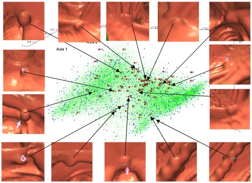
Embeddings of data by DMLLE in low dimensional space spanned by eigenvectors corresponding to the second to the fourth largest eigenvalues. Large dots are true polyps. Medium dots are false positives selected as landmarks. Small dots are nonlandmark samples.

For comparison, we mapped the data to a 3D space by using LLE and plotted the embeddings in Fig. 4. The number of nearest neighbors $K=6$ was used in LLE, which is the same as that used in DMLLE algorithm. It is obvious that positive samples and negative samples aggregate together, which impairs the performance of the classifier. Because LLE focuses on preserving the local geometry of data, it lacks the ability to maintain the global geometry structure of original data in low dimensional space. Especially when data are noisy, faraway data points may be connected by noisy samples and therefore mapped to near place. So most of the data collapse to a central point in the low dimensional space. That is what we observed in Fig. 4.

Figure 4.

Embeddings of data by LLE. Large dots are true polyps. Small dots are false positives.

To show the influence of landmarks on the performance of the DMLLE algorithm, in Fig. 5 we show FROC curves of DMLLE using a different number of landmarks in the training set. We did 100 random samplings for each number of landmarks. For one random sampling, a SVM classifier was trained and tested 100 times in which the experimental configuration was the same as that in Fig. 2. Therefore, each of the following curves is the average of 10 000 FROC curves. The experiments were done on the NIH biowulf computer cluster in parallel mode.²⁵ Figure 5 shows that with an increasing number of landmarks, the performance of DMLLE is also improved. However, when the number of landmarks is greater than 1000, the performance of DMLLE converges. So in the following experiments on the test set, we chose 1000 landmarks for DMLLE to limit the computational burden.

Figure 5.

FROC curves of DMLLE under a different number of landmarks on the training set (polyp size: $6–9\mathrm{mm}$)

To show the advantage of DMLLE on the detection of colonic polyps, in Fig. 6a we show the FROC curves on the testing sets generated by using a bootstrap sampling method on the test set (polyp size: $6–9\mathrm{mm}$). We used the entire training set to train each algorithm; then we generated the testing set for each algorithm and each random run by bootstrap sampling data in the test set. Each point on the curves is the average result of 100 random tests. For clinical purposes, radiologists are concerned most about the sensitivity of the CAD system at low false positives per patient. In Fig. 6b we plot a subregion of the FROC curves. To compare different embedding methods for the nonlandmark samples after using diffusion map on the landmarks, in Fig. 6 we also show the results of the DM Nyström method, which means the nonlandmark samples are mapped to the low dimensional space by the Nyström extension. From them we find that SVM with DMLLE dimension reduction shows higher generalization ability than other methods. In order to show whether the improvement is significant, we compared the sensitivities of five methods at different operation points of FROC curves. We performed t-hypothesis tests (student’s t-test, two-tailed test) to determine whether two samples (x and y) from a normal distribution have the same mean. The standard deviations are unknown but assumed equal. In Table 1 we list the p-value and confidence interval of the t-hypothesis test for DMLLE and other methods at different false positives. By using the t-hypothesis test, we found that the sensitivities of DMLLE between five to ten false positives per patient has significant difference compared with that of the other four algorithms at a significance level of 0.05. That means by using DMLLE, the performance of our CAD system can be improved significantly.

Figure 6.

FROCs of SVM on the large-scale colonic polyp dataset with (no markers) or without (square markers) DMLLE dimensionality reduction, SVM committee (dotted line), SVM using DM Nyström (triangle markers), and SVM using PCA dimension reduction (cross markers). Data are shown for polyps $6\text{to}9\mathrm{mm}$ in size. In (b), the data in (a) is displayed with magnified x-axis scale.

Table 1.

t-hypothesis test of DMLLE with the other four methods on $6–9\mathrm{mm}$ polyps at significance level 0.05. In each item we show the confidence interval of the difference between means of DMLLE and other methods. The p-value for each test is less than 0.001.

False positives	DM Nyström	All features	Committee	PCA
5	[0.0876,0.1119]	[0.2009,0.2230]	[0.1133,0.1352]	[0.0698,0.0918]
6	[0.0947,0.1173]	[0.2193,0.2404]	[0.1275,0.1482]	[0.0802,0.1012]
7	[0.1007,0.1221]	[0.2313,0.2518]	[0.1290,0.1493]	[0.0884,0.1090]
8	[0.1036,0.1239]	[0.2389,0.2582]	[0.1306,0.1492]	[0.0908,0.1099]
9	[0.1056,0.1257]	[0.2447,0.2639]	[0.1217,0.1400]	[0.0912,0.1102]
10	[0.1055,0.1251]	[0.2471,0.2666]	[0.1183,0.1365]	[0.0887,0.1078]

From the experimental result shown before, the DMLLE algorithm shows good performance on the $6–9\mathrm{mm}$ colonic polyp classification. At the same time, we also expect that it works well on the polyps bigger than $9\mathrm{mm}$. In Fig. 7 and Table 2 we show the FROCs and results of t-hypothesis test of the five methods on the bigger polyps $(>9\mathrm{mm})$. The DMLLE method shows again the effectiveness on the bigger colonic polyp classification task. In addition, because the number of $6–9\mathrm{mm}$ polyps in the training set is greater than the number of $>9\mathrm{mm}$ polyps, the performance of DMLLE drops a little for $>9\mathrm{mm}$ polyps compared with that of $6–9\mathrm{mm}$ polyps.

Figure 7.

FROCs of SVM on the large-scale colonic polyp dataset with (no markers) or without (square markers) DMLLE dimensionality reduction, SVM committee (dotted line), SVM using DM Nyström (triangle markers), and SVM using PCA dimension reduction (cross markers). Data are shown for polyps which are greater than $9\mathrm{mm}$ in size. In (b), the data in (a) is displayed with magnified x-axis scale.

Table 2.

t-hypothesis test of DMLLE with the other four methods on polyps bigger than $9\mathrm{mm}$ at significance level 0.05. In each item we show the confidence interval of the difference between means of DMLLE and other methods. The p-value for each test is less than 0.001 except for SVM committee when the false positives are greater than 5.

False Positives	DM Nyström	All features	Committee	PCA
5	[0.0251,0.0591]	[0.1804,0.2192]	[0.0253,0.0568]	[0.0227,0.0580]
6	[0.0277,0.0609]	[0.1760,0.2139]	[0.0045,0.0357]	[0.0261,0.0611]
7	[0.0278,0.0591]	[0.1745,0.2113]	$[-0.0094,0.0200]$	[0.0283,0.0615]
8	[0.0266,0.0579]	[0.1721,0.2086]	$[-0.0038,0.0253]$	[0.0290,0.0614]
9	[0.0270,0.0579]	[0.1719,0.2077]	$[-0.0023,0.0265]$	[0.0304,0.0627]
10	[0.0290,0.0588]	[0.1730,0.2076]	$[-0.0158,0.0119]$	[0.0315,0.0630]

DISCUSSION AND CONCLUSION

We found that the SVM with DMLLE shows better generalizability than SVM with all features, SVM with PCA or DM Nyström dimensionality reduction methods. This result supports our conjecture that we can learn a better classification function in the low dimensional embedding space than in the original high dimensional space. That is also one reason why feature selection methods work. In addition, the advantage of DMLLE over PCA reveals that the colonic polyp data may have a low dimensional manifold structure,^{12, 13, 14} which cannot be discovered by linear dimensionality reduction methods. Although we cannot describe the low dimensional structure definitely, we can still find some clues from the embeddings and figures of true polyps shown in Fig. 3. That means the key factors to discern a true polyp from false polyps are not as many as the features extracted.

In addition, as we mentioned in the previous section, the embedding mechanism of LLE for new samples is in essence a variation of the Nyström extension. The basic Nyström extension will use all landmarks to infer the embedding of a new sample, whereas the LLE will just use the nearest K neighbors. If we view the changing of the size of neighbor region for a new sample as the changing of scale, then it is obvious that the Nyström extension and the LLE compute the embedding for a new sample at different scales. The basic Nyström extension operates at a larger scale and LLE operates at a finer scale. Although LLE works better than the basic Nyström extension, is it the best scale to infer the coordinates of a new sample based on the embeddings of landmarks? It is still an open question and worthy of further exploration.

Since current detection algorithms perform very well on true polyps that are greater than $9\mathrm{mm}$,³ we focused on the detection of true polyps whose sizes are in the range of $6\text{to}9\mathrm{mm}$. To some extent, improving the detection probability of $6–9\mathrm{mm}$ polyps is the main target of current CTC CAD research. In order to compare the performance of different methods, we censored other than $6\text{to}9\mathrm{mm}$ polyps in most our experiments. In addition, according to the comparisons of our DMLLE method with other methods on polyps that are greater than $9\mathrm{mm}$, the DMLLE method also outperformed other methods on bigger polyps. Because the resolution of CTC is limited, the size of polyps will affect the significance of features on the classification task (good features for big polyps may not be significant for smaller polyps.²¹) In practical CTC CAD systems, one could train different classifiers for different sizes of polyps.

In our current experiments, we do not combine the results from supine and prone scans in order to compare the performance of different dimensionality reduction methods. In practical CTC CAD systems, one can get higher sensitivity if the classification of a true polyp is based on supine and prone scans.³ We also do not focus on the detection of adenomatous polyps only but instead consider all histologic types of polyps in our database. Interested readers may find the performance of an SVM committee based on joint classification of adenomatous polyps on supine and prone scans in our previous work.³

In this article, we propose a nonlinear dimensionality reduction method based on diffusion map and LLE for large-scale data. By using Markov transition probability as the measure of distance between samples, diffusion map shows high resistance to noise. Because diffusion map needs to do eigenvalue decomposition for Markov matrix, it limits the application of diffusion map to large-scale data. Inspired by the idea of landmarks in the ISOMAP algorithm, we first randomly select partial data as landmarks. The embeddings of landmarks in low dimensional space is constructed by using diffusion map. These embeddings constitute the global skeleton of whole data in embedding space. Then by using LLE, nonlandmark points are embedded into the same low dimensional space by using nearest landmarks. For any nonlandmark point, the linear geometry relationship with its nearest landmarks is maintained in both high dimensional space and embedding space. By combining global and local dimensionality reduction methods, DMLLE provides a faithful representation of original high dimensional data at coarse and fine scales. As a consequence, it can capture the intrinsic distance relationship between samples and reduce the influence of noisy features. Both of these characteristics are crucial to the performance of classifiers. PCA can be regarded as a global dimensionality reduction method and LLE is a local dimensionality reduction method. In the experiments in our article, we compared the DMLLE with PCA and LLE; the comparison results support our findings.

We applied the proposed DMLLE method to the colonic polyp detection problem on virtual colonoscopy. The embedding of all polyp candidates in 3D space shows that most true polyps concentrate in the valley of two Gaussian-like distributions formed by false polyps. The clustering of true polyps enables the supervised learning method to determine a good decision boundary and achieve higher generalization ability than could be achieved in the original high dimensional space. We compared the test errors of the SVM classifier trained in a low dimensional space by using DMLLE with that of the SVM classifier using all available features. FROC analysis showed that with DMLLE, the SVM classifier shows higher generalization ability than that using all features. DMLLE also shows higher generalization ability compared with an SVM committee using feature selection technology and SVM using PCA linear dimensionality reduction.

References

- Fletcher J. G. and Luboldt W., “CT colonography and MR colonography: Current status, research directions, and comparison,” Eur. Radiol. 10, 786–801 (2000). [DOI] [PubMed] [Google Scholar]
- Frentz S. M. and Summers R. M., “Current status of CT colonography,” Acad. Radiol. 13, 1517–1531 (2006). [DOI] [PMC free article] [PubMed] [Google Scholar]
- Summers R. M., Yao J., Pickhardt P. J., Franaszek M., Bitter I., Brickman D., Krishna V., and Choi J. R., “Computed tomographic virtual colonoscopy computer-aided polyp detection in a screening population,” Gastroenterology 10.1053/j.gastro.2005.08.054 129, 1832–1844 (2005). [DOI] [PMC free article] [PubMed] [Google Scholar]
- Summers R. M., Jerebko A. K., Franaszek M., Malley J. D., and Johnson C. D., “Colonic polyps: Complementary role of computer-aided detection in CT colonography,” Radiology 10.1148/radiol.2252011619 225, 391–399 (2002). [DOI] [PubMed] [Google Scholar]
- Yoshida H. and Nappi J., “Three-dimensional computer-aided diagnosis scheme for detection of colonic polyps,” IEEE Trans. Med. Imaging 10.1109/42.974921 20, 1261–1274 (2001). [DOI] [PubMed] [Google Scholar]
- Acar B., Beaulieu C. F., and Gokturk S. B., “Edge displacement field-based classification for improved detection of polyps in CT colonography,” IEEE Trans. Med. Imaging 10.1109/TMI.2002.806405 21, 1461–1467 (2002). [DOI] [PubMed] [Google Scholar]
- Dijkers J. J., van Wijk C., Vos F. M., Florie J., Nio Y. C., Venema H. W., Truyen R., and van Vliet L. J., “Segmentation and size measurement of polyps in ct colonography,” in Proceedings of 8th International Conference on Medical Image Computing and Computer Assisted Intervention (Springer–Verlag, Berlin Heidelberg, 2005), 3749, pp. 712–719. [DOI] [PubMed]
- Yao J., Miller M., Franaszek M., and Summers R. M., “Colonic polyp segmentation in ct colonography based on fuzzy clustering and deformable models,” IEEE Trans. Med. Imaging 10.1109/TMI.2004.826941 23, 1344–1352 (2004). [DOI] [PubMed] [Google Scholar]
- Paik D. S., Beaulieu C. F., Rubin G. D., Acar B., and Jeffrey R. B., “Surface normal overlap: A computer-aided detection algorithm, with application to colonic polyps and lung nodules in helical CT,” IEEE Trans. Med. Imaging 10.1109/TMI.2004.826362 23, 661–675 (2004). [DOI] [PubMed] [Google Scholar]
- Li J., Franaszek M., Petrick N., Yao J., Huang A., and Summers R. M., “Wavelet method for CT colonography computer-aided polyp detection,” in IEEE 2006 International Symposium on Biomedical Imaging (Arlington, Virginia, 2006). [DOI] [PMC free article] [PubMed]
- Jolliffe I. T., Principal Component Analysis, 2nd ed. (Springer-Verlag, New York, 2002). [Google Scholar]
- Tenenbaum J. B., de Silva V., and Langford J. C., “A global geometric framework for nonlinear dimensionality reduction,” Science 10.1126/science.290.5500.2319 290, 2319–2323 (2000). [DOI] [PubMed] [Google Scholar]
- Roweis S. and Saul L., “Nonlinear dimensionality reduction by locally linear embedding,” Science 10.1126/science.290.5500.2323 290, 2323–2326 (2000). [DOI] [PubMed] [Google Scholar]
- Belkin M. and Niyogi P., “Laplacian eigenmaps and spectral techniques for embedding and clustering,” in Advances in Neural Information Processing Systems 14 (MIT Press, Cambridge, MA, 2002), 585–591. [Google Scholar]
- Coifman R. R., Lafon S., Lee A. B., Maggioni M., Nadler B., Warner F., and Zucker S. W., “Geometric diffusions as a tool for harmonic analysis and structure definition of data part I: diffusion maps and part II: multiscale methods,” Proc. Natl. Acad. Sci. U.S.A. 10.1073/pnas.0500334102 102, 7426–7437 (2005). [DOI] [PMC free article] [PubMed] [Google Scholar]
- Lafon S. and Lee A. B., “Diffusion maps and coarse-graining: A unified framework for dimensionality reduction, graph partitioning and data set parameterization,” IEEE Trans. Pattern Anal. Mach. Intell. 10.1109/TPAMI.2006.184 28, 1393–1403 (2006). [DOI] [PubMed] [Google Scholar]
- Coifman R. R. and Lafon S., “Diffusion maps,” Applied and Computational Harmonic Analysis: Special issue on Diffusion Maps and Wavelets 21, 5–30 (2006). [Google Scholar]
- Fowlkes C., Belongie S., Chung F., and Malik J., “Spectral grouping using the Nystrom method,” IEEE Trans. Pattern Anal. Mach. Intell. 10.1109/TPAMI.2004.1262185 26, 214–225 (2004). [DOI] [PubMed] [Google Scholar]
- Lafon S., Keller Y., and Coifman R. R., “Data fusion and multicue data matching by diffusion maps,” IEEE Trans. Pattern Anal. Mach. Intell. 10.1109/TPAMI.2006.223 28, 1784–1797 (2006). [DOI] [PubMed] [Google Scholar]
- Bengio Y., Paiement J. F., Vincent P., and Delalleau O., “Out-of-sample extensions for LLE, ISOMAP, MDS, eigenmaps, and spectral clustering,” in Advances in Neural Information Processing Systems (MIT Press, Cambridge, MA, 2004), 307–311. [Google Scholar]
- Yao J., Summers R., and Hara A., “Optimizing the committee of support vector machines (SVM) in a colonic polyp cad system,” in Medical Imaging 2005: Physiology, Function, and Structure from Medical Images (SPIE, 2005), 5746, pp. 384–392.
- Burges C. J. C., “A tutorial on support vector machines for pattern recognition,” Data Min. Knowl. Discov. 10.1023/A:1009715923555 2, 121–167 (1998). [DOI] [Google Scholar]
- Li J., Yao J., Summers R. M., Petrick N., and Hara A., “An efficient feature selection algorithm for computer-aided polyp detection,” International Journal on Artificial Intelligence Tools 15, 893–916 (2006). [Google Scholar]
- Fukumizu K., Bach F. R., and Jordan M. I., “Dimensionality reduction for supervised learning with reproducing kernel hilbert spaces,” J. Mach. Learn. Res. 25, 73–99 (2004). [Google Scholar]
- Biowulf linux cluster, National Institutes of Health, Bethesda, Md. (http://biowulf.nih.gov).