Hydrodynamics of the escape response in bluegill sunfish, Lepomis macrochirus

SUMMARY

Escape responses of fishes are one of the best characterized vertebrate behaviors, with extensive previous research on both the neural control and biomechanics of startle response performance. However, very little is known about the hydrodynamics of escape responses, despite the fact that understanding fluid flow patterns during the escape is critical for evaluating how body movement transfers power to the fluid, for defining the time course of power generation, and for characterizing the wake signature left by escaping fishes, which may provide information to predators. In this paper we present an experimental hydrodynamic analysis of the C-start escape response in bluegill sunfish (Lepomis macrochirus). We used time-resolved digital particle image velocimetry at 1000 fps to image flow patterns during the escape response. We analyzed flow patterns generated by the body separately from those generated by the dorsal and anal fins, to assess the contribution of these median fins to escape momentum.

Each escape response produced three distinct jets of fluid. Summing the components of fluid momentum in the jets provided an estimate of fish momentum that did not differ significantly from momentum measured from the escaping fish body. In contrast to conclusions drawn from previous kinematic analyses and theoretical models, the caudal fin generated momentum that opposes the escape during stage one, while the body bending during stage one contributed substantial propulsive momentum. Additionally, the dorsal and anal fins each contributed substantial momentum. The results underscore the importance of the dorsal and anal fins as propulsors and suggest that the size and placement of these fins may be a key determinant of fast start performance.

INTRODUCTION

The escape response (also called a C-start, fast-start, or Mauthner startle response) of fishes is perhaps the best-studied behavior in vertebrates, and has been analyzed from a broad array of perspectives using a diversity of techniques. A large number of studies have focused on the neural connections that underlie the startle response and have mapped the neuronal circuitry that is important in producing the escape behavior, which is primarily generated by large paired reticulospinal neurons called Mauthner cells (reviewed in Eaton et al., 2001; Korn and Faber, 2005). These cells trigger a strong, mostly unilateral contraction of axial muscle that bends the body into a ‘C’ shape, which is then typically followed by one or more alternating tail beats. Numerous studies have described both the characteristic pattern of muscle activity (e.g., Ellerby and Altringham, 2001; Jayne and Lauder, 1993; Westneat et al., 1998) and the kinematics (reviewed in Domenici and Blake, 1997; Wakeling, 2006). Most of these studies divide the behavior into at least two major components: stage one, the initial ‘C’ bend, and stage two, the stroke during which the body bends out of the ‘C’ shape (Weihs, 1973).

Because escape responses are used to flee predators, escape performance has clear fitness consequences. Therefore, studies of fish fast-start responses have also served as a key component of evolutionary and ecological studies of predator-prey interactions (e.g., Bergstrom, 2002; Domenici et al., 2008; Gibb et al., 2006; Langerhans et al., 2004). Indeed, fish that execute slower or less effective escape responses are eaten preferentially over individuals that have higher escape performance (Walker et al., 2005).

One area in which escape responses are poorly understood is the pattern of water flow generated during the escape: how is power transferred from body muscles into the surrounding fluid? In particular, what proportion of the total power is transferred during the stage one C bend, relative to the following tail beat? Stage one has often been called “preparatory” (starting with Weihs, 1973), suggesting that it does not power the final escape. Others have objected to such terminology (Wakeling, 2006) on the basis of theoretical calculations that show thrust during stage one. This argument is not purely semantic; the division of power among the stages has implications for both neural control and performance. Specifically, if substantial thrust is produced during stage one, then the Mauthner circuit that controls stage one also has a direct effect on overall escape performance, and the whole body, which contributes to the C bend, is critical for force production. However, if stage two is dominant, then the Mauthner circuit is more like a trigger for a behavior in which other circuits may have a greater impact on performance. In this case, because stage two involves more caudal fin movement than body movement (Domenici and Blake, 1997), the caudal fin would be more important for force output than the rest of the body.

Therefore, the goal of this study is to contribute a comprehensive, experimental analysis of the fluid dynamics of C-start escape responses in a teleost fish, the bluegill sunfish Lepomis macrochirus, and to present a description of the patterns of fluid momentum that result from escape responses. Our fluid dynamic data directly indicate the relative importance of stage one and two for force production, along with the contributions of the dorsal and anal fins to thrust production during the escape response. These data are particularly valuable for understanding the time course of locomotor power generation by escaping fish, for correlating fluid dynamic phenomena with previously well-characterized C-start kinematics, and for characterizing the wake signature of escaping fish, which is important for predators which may use this signature to track fish (see e.g., Hanke and Bleckmann, 2004; Hanke et al., 2000).

METHODS

Fish

Bluegill sunfish (Lepomis macrochirus Rafinesque) were collected with nets in ponds near Concord, MA. Animals were maintained at room temperature (∼20 °C) in separate 40 l freshwater aquaria with a 12:12 hour photoperiod, and were fed earthworms three times weekly. Juveniles were used for flow visualization experiments. After experiments were completed, each fish was lightly anesthetized using buffered MS222 (0.2 g l^-1), digitally photographed, weighed, and total length L was measured. The four individual bluegill used for kinematic and flow visualization analysis had mean total body length L = 11.0±0.4 cm (S.E.M.) with a range from 9.7 to 13.3 cm. Mean body mass was 21±2 g. In total, 21 escape responses were analyzed, with at least four sequences per individual.

Mass distribution

To determine both longitudinal and dorso-ventral mass distribution, juvenile bluegill of similar size to those used in flow visualization experiments were euthanized with an overdose of buffered MS222. Individuals were frozen at -20°C, then weighed and photographed. Each animal was sectioned into either transverse or frontal slices using a standard bandsaw with a fine-toothed blade (approximately 1 mm thickness). For transverse sections, animals were cut approximately at the posterior margin of the eye, through the pectoral fin base, posterior to the pelvic fins, through the base of the dorsal and anal fins, and at the end of the hypural bones in the caudal fin (Lauder, 1982). For frontal sections, animals were sectioned at the base of the dorsal fin, though the center of the peduncle, and at the base of the anal fin. Sections were then weighed individually and photographed from lateral and both cross-sectional views (i.e., the cut surfaces on the anterior and posterior sides for transverse sections, or the dorsal and ventral sides for horizontal sections). The sum of the mass of the sections was subtracted from the total fish mass to determine the mass lost to the bandsaw. Mass per unit length was then estimated by interpolating 20 evenly spaced points from the snout to the tail, assuming that mass is zero at the tips of the snout and tail, and was normalized to the total mass of the fish and the total length. Mass per unit height was estimated in the same way for frontal sections along the height of the fish.

Five individuals were used to estimate the mass distribution of bluegill. The mean total body length of these fish was 10.9±0.7 cm (S.E.M.) with a range from 10.6 to 11.3 cm. Mean body mass was 22.5±0.3 g. Three of these individuals were sectioned transversely and two were sectioned frontally.

Experimental protocol

Experiments were performed in a recirculating flow tunnel (600 l) with a 28 cm × 28 cm × 80 cm working section used in previous experiments on fish locomotor hydrodynamics (e.g., Tytell and Lauder, 2004; Tytell et al., 2008). A low flow speed was used (∼0.7 L s^-1) to orient the fish consistently using the rheotaxis response, and this greatly aided in positioning the fish within the laser light sheet. This orientation swimming speed was in the range in which bluegill swim using only their pectoral fins, and has been shown not to affect the kinematics of the escape response (Jayne and Lauder, 1993). Animals were gently maneuvered into the center of the working section using a wooden dowel, which was removed prior to filming an escape. Escape responses were elicited by dropping into the tank a weight with a flat plate (approximately 5 cm diameter) attached to the bottom to generate an impulsive “slap” on the water surface. The weight was secured with a string so that it dropped just below the surface of the water and produced a pressure wave (known to elicit escape responses; Eaton and Emberley, 1991; Tytell and Lauder, 2002) but did not disturb the flow substantially in the region of the fish. The string also ensured that the stimulus dropped in a consistent location, anterior and to the right of the fish (see Fig. 1B). This stimulus was effective at inducing escape responses in bluegill.

Fig. 1.

(A) Top view of filming and laser configuration, approximately to scale. Laser light sheets from two lasers (‘laser 1’ and ‘laser 2’) oriented at 90° to each other were used to avoid shadows. Particle motion was filmed from below. The ventral camera is not shown, but its field of view is indicated by a square. Both cameras acquired images synchronously at 1000 fps, with 1024 × 1024 resolution. The location of the stimulus is shown with a white circle. A lateral camera was used to determine the position of the fish in the light sheet. A slow flow from left to right was used so that the fish would maintain a consistent orientation. (B,C) Example images from the ventral camera (B) and lateral camera (C). Note that in the lateral view (C), only a portion of the fish’s upper body can be seen in the bright laser light.

Imaging and flow visualization

Figure 1 shows the imaging and flow visualization experimental arrangement. Two cameras were used to image the C-start behavior. One camera (labeled ‘ventral camera’ in Fig. 1; Photron APX, Photron USA, Inc., San Diego, CA, USA) viewed the fish from below through a front surface mirror at a 45° angle (Fig. 1B). The camera was calibrated across the full spatial field of view with DaVis 7.1 software (Lavision, GMBH) using an evenly spaced grid of points, which allowed compensation for any spherical distortion introduced by the camera lens and mirror. The second camera, synchronized electronically with the ventral camera (labeled ‘lateral camera’ in Fig. 1; Photron FastCam) viewed the fish from the side with a slight downward tilt which allowed quantification of the position of the laser light sheet on the body of the bluegill (Fig. 1C). All imaging was performed at 1000 frames s^-1 (fps). At this frame rate, the ventral camera had a pixel resolution of 1024 × 1024, while the lateral camera had a resolution of 1280 × 512.

Two Coherent I310 10 Watt argon-ion lasers were used simultaneously to illuminate neutrally buoyant 12μm diameter silver-coated glass beads (density 1.3 g cm^-3; Potter Industries, USA) in the region surrounding the fish. Laser light from each laser was spread into a horizontal sheet using cylindrical lenses. Light from one laser was reflected off a mirror in the tank to produce a light sheet oriented at 90° to the other (Fig. 1A). This configuration minimized shadows during the escape behavior (Fig. 1B) and allowed a near full-field analysis of water flow patterns during the escape. Where the two light sheets overlapped, particle illumination was brighter, but illumination provided by a single laser as seen in the darker regions of the imaged area (Fig. 1B) was sufficient for data analysis. As a result of the orientations of the two laser light sheets, only in very small areas near parts of the highly curved body was no illumination present, and water flow patterns during the C-start could be analyzed for nearly the full image. This arrangement thus prevented the large shadows that would otherwise be cast by the bending fish from prohibiting analysis in large regions of the image. Fluid flow patterns were estimated from the ventral video using standard multiple pass particle image velocimetry algorithms (Hart, 2000; Willert and Gharib, 1991), performed using DaVis 7.1 software as in our previous research (e.g., Lauder and Madden, 2007; Tytell, 2006). This yielded a matrix of 175 by 175 vectors calculated for each image in the C-start sequence for a total of 30,625 vectors per image. Approximately 200 images per sequence were recorded to provide full coverage of flows throughout the entire C-start and at least the first full tail beat after the escape response proper.

Three sets of separate experiments were conducted on all individuals with the laser light sheet oriented first at mid-body, then intersecting the fish at the dorsal fin and tail, and finally intersecting the fish at the anal fin and tail. The location of the light sheet on the body was determined from the lateral view camera (Fig. 1C). This allowed separate analysis of whole body flows as well as the fluid flow patterns generated by the dorsal fin and the anal fin. Due to slight variations in fish position in the light sheet when the C-start was elicited, data from the body were divided into upper body and lower body analyses. Figure 2 shows the number of hydrodynamic sequences collected with the laser light sheets at four approximate positions along the dorso-ventral body axis: through the dorsal fin, the upper body, the lower body, and the anal fin. The largest number of sequences (11) were for the lower body, which included most of the caudal peduncle and the fork of the caudal fin.

Fig. 2.

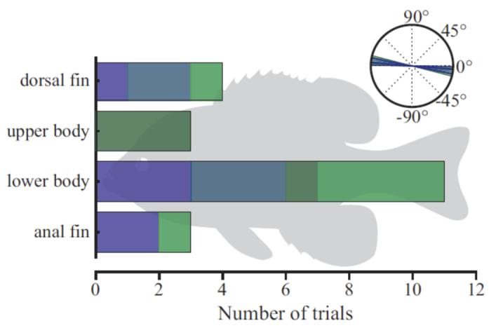
Number of trials with the laser light sheet at four different dorso-ventral positions. Light sheet height was measured at half the fish’s body length at the end of stage one. Inset shows the light sheet angles which varied slightly as individual fish were slightly tilted in some of the sequences. Different colors represent different individuals. A silhouette of the fish is shown in the background as a guide to the light sheet positions, so that the width of each bar represents the approximate range of positions.

Kinematics

Midlines were digitized manually from the ventral video using custom software in Matlab R2006b (Mathworks, Natick, MA, USA). Approximately 12 points were identified along the ventral center line of the body. Points were then smoothed using a smoothing spline that produced the smoothest interpolant to the points with a mean squared error (MSE) of approximately 0.25 pixels² (Walker, 1998) and 20 evenly spaced points were interpolated.

Stages of the escape response were defined according to the angular velocity of the head, using standard definitions (Domenici and Blake, 1997). Angular velocity of the head was determined by calculating the angle of the segment from the tip of the snout to the fourth point (near the posterior margin of the operculum) and taking a numerical derivative with respect to time using a second-order central difference algorithm (Press et al., 1992). Stage one, in which the fish bends into a C shape, was defined to be the period from the first visible motion of the tip of the snout until the angular velocity of the head changed sign (for a sample plot, see Fig. 4). Since all turns were to the fish’s left due to the consistent location of the stimulus relative to the fish body, stage one was thus the time period in which the head was moving to the fish’s left. Stage two was the period from the end of stage one until the head’s angular velocity went to zero or changed sign again (i.e., the period when the head was moving to the fish’s right). Stage one duration is represented by Δt₁; stage two duration is Δt₂; and the total duration of the escape is T (= Δt₁ + Δt₂).

Fig. 4.

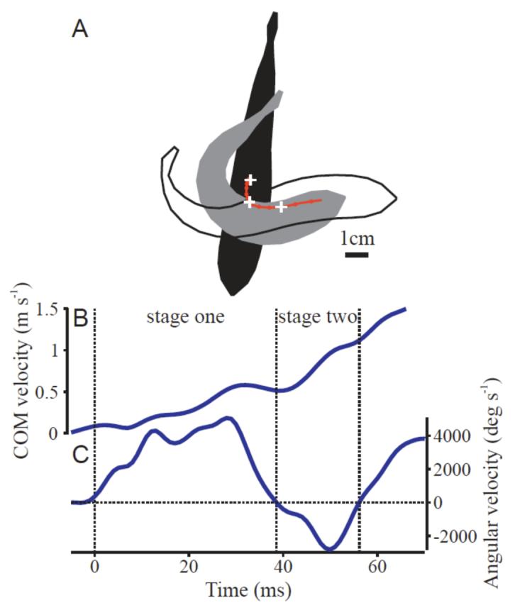
Kinematics from a typical C-start. (A) Silhouettes of the body in its initial position (black), at the end of stage one (gray) and at the end of stage two (white). The location of the center of mass over time is shown with a red line with dots every five milliseconds. White crosses mark the initial position, stage one and two positions. (B) Velocity of the center of mass over time. Divisions between stage one and two are shown with dotted lines. (C) Angular velocity of the head over time.

The true center of mass (COM) position was determined by integrating the x and y coordinates of the midline multiplied by the mass per unit length (estimated above) as a function of position along the arc of the midline. The final angle of the COM trajectory was determined by fitting a line to the COM position in at least 10 frames at the end of stage two. COM velocity was estimated by fitting a smoothing spline (MSE = 0.125 pixels²) and taking the time derivative of the spline. Total fish momentum M_body was estimated by multiplying the fish’s mass by the COM velocity. At each instant in time, fish momentum was divided into components parallel and perpendicular to the final trajectory angle. At the end of stage two, all of the fish’s momentum is by definition parallel to the final trajectory, and is therefore represented by the symbol M.

Lateral images (Fig. 1C) were used to estimate the position and angle of the light sheet on the fish’s body by noting anatomical landmarks that were illuminated by the laser (such as the tip of the snout and the upper margin of the caudal peduncle) and measuring the position of those landmarks on a still, lateral image of a bluegill sunfish. Escape responses were divided into four classes according to where the light sheet intersected the fish’s body: dorsal fin, upper body, lower body, and anal fin (Fig. 2).

Fluid flow analysis

Background fluid velocity $\stackrel{‒}{\mathbf{u}}$ was determined by manually identifying a small region far from the fish prior to the C-start and determining the mean of both streamwise and cross-stream flow velocity in that region. Mean velocities were then subtracted from the flow fields.

Inspection of the high-speed videos revealed three distinct jets of water produced by each C-start. These three fluid jets were easily indentified manually in each sequence. Using custom software in Matlab, ellipsoidal regions J_i were drawn around the fluid flow in each jet i. Jet 1 was defined to be the first jet formed, produced by the tail during stage one. Jet 2 was generated approximately in the opposite direction as jet 1, and was initially produced along the body in stage one and the tail in stage two. Jet 3 was approximately 90° to jet 2 and formed during stage two.

For each jet i, the fluid momentum per unit height μ_jet,i was determined by integrating fluid velocity over the ellipsoidal region:

$${\mu }_{\mathit{jet},i}=\rho {\int }_{J_i}\int (\mathbf{u}-\stackrel{‒}{\mathbf{u}})dA,$$ (1)

where ρ is fluid density, u is the velocity vector, $\stackrel{‒}{\mathbf{u}}$ is the mean velocity, dA is a unit of area, and J_i is the ellipse the surrounds the jet. Effectively, this integral takes the average flow vector in the ellipsoid and multiplies it by the area of the elipse and the density of water.

Because PIV only produces flow velocities in a plane, μ_jet,i has units of momentum per unit height. To estimate the total jet momentum in three dimensions, we must account for two points: (a) given the same movement, larger fins will produce larger jets, and (b) because the light sheet intersects a two-dimensional slice, not all of the jet will be visible. To account for point (a), note that each jet is produced by a different section of the fish’s body: jet 1 by the caudal fin and jets 2 and 3 by the body. The dorsal or anal fins could also contribute to jet 2 in trials with the light sheet at the level of each fin. In this case, the contribution is referred to as the “dorsal fin jet” or “anal fin jet.” As a general term, we will refer to the fins or body, when used to generate a jet, as an actuator surface, and we will denote their lateral area by A_i, for the surface that produces jet i. To account for point (b), note that μ_jet,i will depend on the level of the PIV light sheet. For instance, if the sheet is closer to the midline, it will intersect a longer section of the caudal fin actuator surface than if the sheet is more dorsal, and μ_jet,i will be correspondingly larger. We will use l_i(z) to denote the length of the actuator surface at the level z of the light sheet on the fish’s body. Note that l_i(z) does not depend on the jet flow direction or the position of the jet ellipsoid, but only on the level of the light sheet on the fish’s body (as determined from the lateral camera; Fig. 1C). Thus, as a first approximation of the 3D structure, the total momentum M_jet,i in jet i should be proportional to the momentum per unit height, scaled by the total area of the actuator surface (point a) and the length of the surface intersected by the PIV plane (point b), as follows:

$${\mathbf{M}}_{\mathit{jet},i}={\mu }_{\mathit{jet},i}\frac{A_i}{l_i\left(z\right)},$$ (2)

For simplicity, the scaling factor l_i(z) was determined for the light sheet level z at the end of stage one, rather than the time-varying height. Note that both M_jet,i and μ_jet,i are vectors and can be decomposed into components parallel and perpendicular to the final trajectory. Force was estimated from the time derivative of M_jet,i. Fluid momentum is normalized throughout by dividing by the final fish momentum M, and force is normalized by dividing by the average force required to produce the final momentum, M / T.

RESULTS

Mass distribution

Masses of the bluegill sections relative to the total body mass are shown in Fig. 3A and B. The mass per unit area for the lateral surface was estimated by multiplying the two distributions (Fig. 3C). The density of the fish was very close to water in all sections (data not shown); variation among fish and sections precluded a more quantitative analysis of density.

Fig. 3.

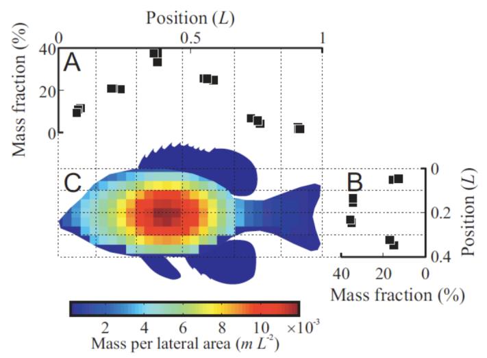
Distribution of fish mass. (A, B) Fraction of total fish mass in transverse (A) or horizontal (B) slices. Dotted lines indicate the approximate thickness of each slice. (C) Estimated mass distribution across the fish body. Color indicates the mass per lateral area, normalized by the fish’s mass m and the length L.

Kinematics

An example C-start is shown in Fig. 4, and mean kinematic values all behaviors analyzed are presented in Table 1. Due to the controlled placement of the stimulus, behaviors were quite consistent. Different individuals did not have significantly different kinematics (one-way MANOVA on 11 kinematic variables; Wilk’s λ = 0.016; χ² = 47.4; df = 33; P = 0.051), although the P value was close to significance indicating that there was a trend toward systematic differences in C-start kinematics among individuals. Stage one durations were nearly twice that of stage two, and peak COM velocity during the escape response was nearly three times that at the end of stage one (Table 1).

Table 1.

Mean escape response kinematics

	Mean	SEM	Units
Stage one duration	34.7	± 0.2	ms
Stage two duration	18.2	± 0.2	ms
Peak angular velocity	3150	± 20	deg s-1
Total turn angle	104	± 1	deg
COM velocity at the end of stage one	4.81	± 0.07	L s-1
Peak COM velocity	12.4	± 0.1	L s-1

See text for explanations of variables. N = 21 escapes (4 individuals). SEM, standard error of the mean. L, total body length.

Flow structure

Three fluid jets were identified in each escape response, and figures 5 and 6 show the development of fluid momentum in the jets. These jets represent momentum added to the water as a result of body and fin movements during the escape response. Jet 1 was formed by the tail during the initial C bend in stage one (Fig. 5A,B; see also supplementary video 1) and was fully developed during stage two (Fig. 5C). Jet 2 was initiated during stage one and was formed by the body at the center of the C bend (Fig. 5B). As the body began to turn after stage one, the tail continued to add momentum until the end of stage two. At the end of stage two, momentum in jet 2 was fully developed (Fig. 5C,D). Jet 3 developed near the mid-body region during stage two and afterwards, on the opposite side as jet 2 (Fig. 5C, D). This jet was often more diffuse than jets 1 or 2. Thus, by the conclusion of the escape response, three well-developed fluid jets had formed, and these jets are nearly orthogonal to each other (Fig. 5).

Fig. 5.

Images of a typical bluegill sunfish C-start showing the associated hydrodynamic flows at the mid-body level (yellow velocity vectors). Note that only every 4^th vector is shown for clarity. The stimulus is visible in the lower left of each panel, and the three dominant jet flows are labeled (see text for discussion). The strong suction on the inside of the C-bend is clearly visible in panel B. Note that jet 1 represents momentum that largely opposed the fish momentum along the final trajectory. Vectors in the region of the stimulus in the lower left corner of each panel and over the fish body have been deleted. Bluegill icon at the bottom indicates the position of the light sheet (black line) in this sequence and a time-line for this sequence is shown. Peak flow velocities are nearly 1 ms^-1. In this escape, stage one lasted for 32ms and stage two for 25ms, so that the whole escape lasted 57ms.

Fig. 6.

C-start escape responses showing flows resulting from motion of the dorsal (A) and anal (B) fins. Bluegill icons at the top of each panel indicate the position of the light sheet (black line) for each panel. The stimulus generating the escape was just off the lower left corner of each image. Both images are from the end of stage one. (A) Jet 1 and the dorsal fin portion of Jet 2 are shown. The protruding fin is the anal fin. (B) The anal fin portion of jet 2 is shown. Jet 1 is not visible because the light sheet for this trial was located just below the caudal fin. In both panels, every second vector is shown for clarity.

The dorsal and anal fins also contributed momentum during the C-start. Light sheets at the level of the two fins indicated that they added momentum to jet 2 (Fig. 6). These jets were likely continuous with jet 2, but they were treated separately in the analysis to quantify the importance of these two fins. The sharp trailing edge of the dorsal and anal fins produced a distinct starting vortex center as flow separates from the training fin edge in stage one. Additionally, the soft dorsal and anal fins tended to flick out at the end of stage two, adding additional momentum to this jet.

Fig. 7 shows the development of vorticity in the flow field, as well as the identified boundaries of the jets. Two well-defined counter-rotating vortices were shed with jet 1 (Fig. 7C), suggesting that it is a vortex ring. Jet 2 had less clear vortices. Instead, as the tail swept around through stage two, it produced shear layers of opposite sign on either side of the jet (Fig. 7D, E). These shear layers were unstable and tended to break up into multiple vortices (Fig. 7F). Finally, because jet 3 was fairly diffuse, it was rarely accompanied by clearly defined vortical structures.

Fig. 7.

(previous page) Flow and vorticity for a fast start with the light sheet intersecting the lower body. Vectors show the flow with brighter green colors indicating high velocity. Red and blue colors indicate counter-clockwise and clockwise vorticity, respectively. Dashed ovals with numbers show the outlines of identified jets. The fish silhouette is shown in gray. The inset shows the light sheet position on the body. The time starting from the first visible movement is shown at the top of each panel, and a time-line for this escape is shown at the bottom right.

Conservation of momentum dictates that the total momentum in the system must remain constant. Because the fish momentum plus the fluid momentum was zero at the beginning of the behavior, the total must also be zero at the end of the behavior. Thus, the momentum in the jets represented the reaction force on the fish over the course of the escape response and must be equal and opposite to the fish’s momentum. Fig. 8 shows how the fluid momentum was divided among the jets, and how it compared to the total fish momentum. Fig. 8A shows momentum parallel to the fish’s final trajectory, normalized by the fish momentum M at the end of stage two. Most fluid momentum was contained in body jet 2, although both the dorsal and anal fin contributed substantially. The column labeled ‘all jets’ is the sum of the mean magnitudes of each jet. Error was estimated in the standard way by propagating the standard error for each jet’s mean in quadrature (Taylor, 1982). Mean total fluid momentum was not significantly different from the fish’s momentum M (t = 0.464; df = 3; P = 0.67), as predicted by conservation of momentum. However, the fluid momentum perpendicular to the final trajectory, summarized in Fig. 8B, was significantly different from zero (t = 9.599; df = 3; P = 0.002). This result, which is contrary to the predicted conservation of momentum, was most likely due to the fact that the momentum estimates were made at the end of stage two, but jet 3 generally continued growing after stage two. The relatively narrow field of view needed to visualize escape response flow patterns precluded a detailed analysis of the momentum in jet 3, but its growth would tend to push the perpendicular fluid momentum closer to zero.

Fig. 8.

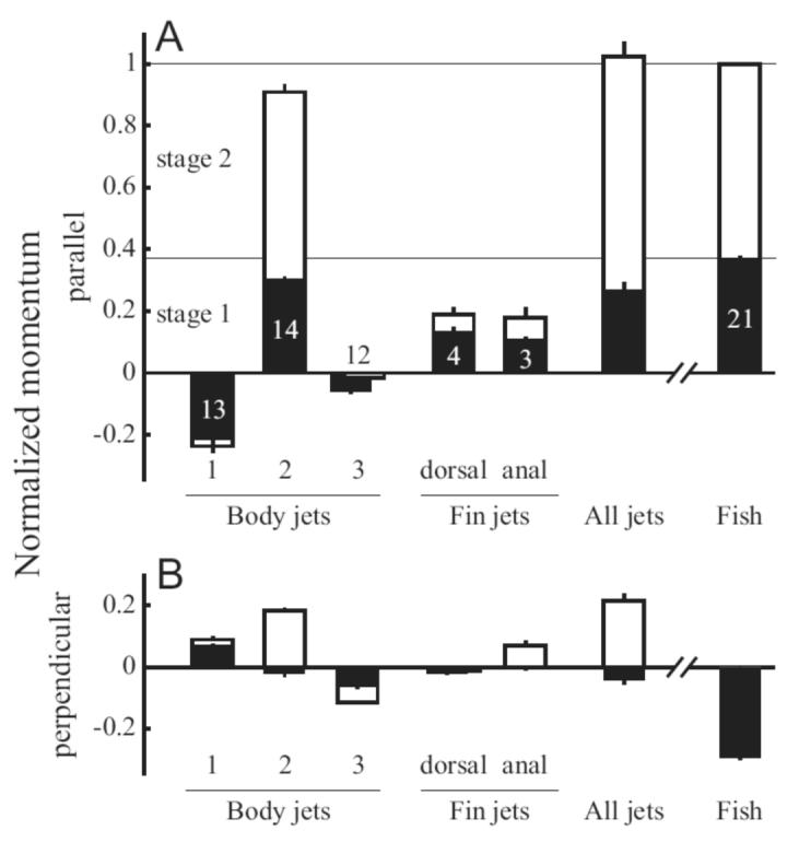
Fluid momentum matches the fish momentum parallel to the final trajectory. Momentum in each jet is shown for stage one (solid bars) and stage two (open bars) with error bars representing standard error. Numbers in each bar represent the number of sequences used to estimate momentum and are the same for both parallel (A) and perpendicular (B) estimates. The bar labeled “All jets” represents the sum of the mean momentum values for each body jet and the dorsal and anal fin jets. Momentum is scaled to the fish’s momentum M at the end of stage two. A: Momentum parallel to the final fish trajectory. The bars for jet 3 are shown offset from one another to indicate that momentum in that jet decreased from stage one to stage two. B: Momentum perpendicular to the final fish trajectory. Note that the perpendicular fish momentum at the end of stage two is zero by definition, so no open bar is shown.

A substantial amount of the total momentum was produced during stage one. By the end of stage one, the fish’s momentum was 37.2±0.6% of its total momentum at the end of stage two. The reaction force for this acceleration was mainly represented by jet 2, which contained 30.4±0.8% of the total momentum by the end of stage one (Fig. 8A, filled bars). Additionally, the force producing the dorsal and anal fin jets mostly occurs during stage one. Together, they produce 24±2% of the fish’s total momentum by the end of stage one and 37±4% by the end of stage two.

To examine the timing of force production in more detail, Fig. 9 shows the time derivative of jet 2 momentum, which is an approximation of the force producing the jet. Such force traces typically had two peaks, one in each stage. Fig. 9A shows an example trace. So that different sequences can be compared, force was nondimensionalized by dividing by the average force required to produce the final fish momentum (M / T; an example is shown with the dashed line in Fig. 9A). Fig. 9B shows the mean force peaks from each stage. The first peak occurred 27.9±0.8% of the way through stage one, or 9.3±3 ms after the first movement, while the second was 56±1% through stage two, or 46.0±0.4 ms after the first movement. In nondimensional force, the average height of the two peaks were 0.45±0.01 and 2.23±0.07. On average, peak forces in stage 2 were 6.2±0.5 times peak forces in stage one (range 2.2 to 17.7).

Fig. 9.

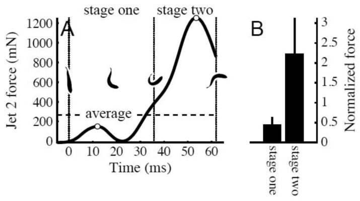
The force that produced jet 2 (i.e., the change in jet 2 momentum) typically had two peaks, one in stage one and another in stage two. (A) Example force trace showing the two peaks, identified with open circles. Stage one and two are separated by dotted lines. Outlines showing body conformation during the c-start are shown in the middle of the graph. The average force required to give the fish its final momentum is shown as a dashed line. Time zero is the time of first visible movement. (B) Mean values of the stage one and two peak forces (open circles in panel A) for all trials. Force has been normalized by the average force (dashed line in panel A) for each trial.

Fig. 10 shows a summary of the jet positions and angles, along with the fish’s momentum and direction. Blue vectors represent the momentum M_jet,i for each jet i. Their bases are at the mean position for each jet, and the overall mean jet momentum and angle is given by a black vector. Red vectors show the total fish momentum. The lengths of all vectors were normalized to the total fish momentum at the end of stage two, which is why all the red vectors in Fig. 10E are the same length. Jets 1 and 2 were generally parallel to the final trajectory and represented reaction forces opposing and aiding the escape, respectively. Jet 3 was mostly perpendicular to the final trajectory, and appeared to represent a reaction force counteracting the angular momentum of the turn.

Fig. 10.

Summary of jet and fish momentum for body trials. Jets are shown in blue; each line represents the magnitude and angle of a jet, radiating from the mean position of the jet. Mean angle and momentum is shown with a black arrow. Fish momentum is shown in a similar way, with red lines radiating from the fish’s center of mass and a black arrow to indicate the mean. Fish silhouettes are shown in gray. All vectors are scaled as a fraction of the final fish momentum at the end of stage two (panel E). Data are for body jets, as indicated by the inset.

Jet 1 was perpendicular to the initial fish orientation (Fig. 10A, B). Thus, it might appear that jet 1 indicated a reaction force that starts the initial rotation of the turn. However, the data did not support that hypothesis. Linear regression revealed that there was no significant relationship between peak angular velocity and total jet 1 momentum (P = 0.134; data not shown).

The fluid momentum data indicated a performance gradient associated with perpendicular momentum. Turns with more fluid momentum perpendicular to the final trajectory had significantly lower final velocities. Fig. 11 shows the final fish momentum plotted against the perpendicular fluid velocity component as a fraction of the total fluid momentum. Linear regression indicated a significant negative relationship (P = 0.029).

Fig. 11.

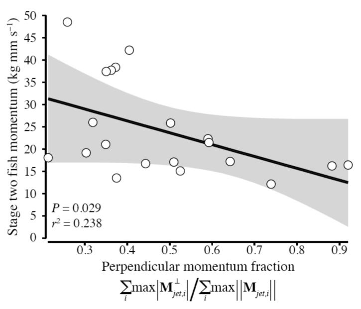
Fluid momentum perpendicular to the fish’s final trajectory reduces the fish’s total momentum. The fish momentum at the end of stage two is plotted against the fraction of perpendicular jet momentum in the total momentum. $M_{\mathit{jet},i}^{\perp }$ is the perpendicular component of jet momentum, and the operators max(·) and ∥·∥ indicate the maximum value over time and the vector magnitude, respectively.

DISCUSSION

Fluid dynamics of the C-start

We were surprised to discover that each C-start escape response of bluegill sunfish produces three distinct, roughly orthogonal, jets of fluid from the mid-body region, as the existing kinematic literature on C-starts did not lead us to expect this pattern of fluid flow. Our unpublished data on two other species (zebrafish Danio rerio, and brook trout Salvelinus fontinalis) also show that these same three jet flows are produced with each C-start. The hydrodynamic patterns presented in this paper are thus not unique to bluegill, and we suspect that the fluid flows described here are produced during escape responses in most teleost fish with a relatively generalized perch-like body morphology. Our results also show a substantial active contribution of momentum from the dorsal and anal fins, which supports our previous results showing that these fins contribute actively to swimming (Jayne et al., 1996; Tytell, 2006; Tytell et al., 2008).

Fish momentum along the escape trajectory quantitatively matches the summed momentum of the three identified hydrodynamic jet flows plus the dorsal and anal fin flows (Fig. 8A), suggesting that our analysis has captured the major hydrodynamic events contributing to the escape. Jet 1 is generated by the caudal fin area of the fish, and the bulk of the jet 1 momentum opposes the escape trajectory. Production of this jet, which would act to reduce the efficiency of the escape response, may be an unavoidable consequence of having a flexible body bending into a C shape. Fluid will naturally separate from the sharp trailing edge of the fish tail as the body bends and the tail moves toward the head, resulting in a distinct jet as the tail decelerates at the end of stage one.

Jet 2, which is first formed in stage one and continues developing through stage two, contributes the bulk of escape trajectory momentum (Fig. 8A). Bending of the body into the C shape produces a large suction region on the inside curve of the body which in turn produces a large bulk flow in a direction generally opposite to that of the final escape trajectory, and hence opposite to the direction of Jet 1. The importance of the suction region is clearly seen in the vector fields calculated for stage one (Fig. 5B; Supplementary video 1) where the side motion of the mid-body region has induced a large diameter high-velocity jet. Much lower flows are visible on the pressure side of the bending body.

Finally, jet 3 contains much less momentum along the final escape trajectory than either jet 1 or jet 2, and has a mean direction that is largely perpendicular to the escape (Fig. 8B; Fig. 10). Examination of the flow velocity field (Fig. 5C, D) in the region of jet 3 shows that this jet is oriented in a largely perpendicular direction to jets 1 and 2, and is generated by bending along the posterior half of the body during stage two. The momentum in this jet may contribute to steering the fish out of stage one and into stage two by countering angular momentum generated during the C-bend phase of the escape. Alterations of body bending during stage two may allow adjustment of the final escape heading, but our data show that momentum allocated to directions orthogonal to the final trajectory decreases escape performance overall. The escapes with the highest stage two momentum have the lowest fraction of momentum perpendicular to the final trajectory (Fig. 11).

Our experimental setup deliberately controlled as much as possible for initial body orientation and stimulus location, and so variation in the direction taken by escaping fishes was low. Future studies could induce a diversity of escape directions and profitably compare the directions of each jet, particularly jet 3, with the final escape direction. We hypothesize that the angle of jet 3 will be strongly correlated with the final turn angle.

One key finding of our study is that a substantial portion of jet 2 is generated during stage one (Fig. 8A). Even though the COM moves relatively little during stage one, the forces and accelerations are high and contribute to the final escape performance. This result indicates that stage one is not well-described as a “preparatory” phase, followed by the “propulsive” phase two (initially by Weihs, 1973). These terms have been persistent in the fast-start literature (e.g., Frith and Blake, 1995; Harper and Blake, 1990; Muller et al., 2008; Tytell and Lauder, 2002), even though various researchers have argued against them (see review by Wakeling, 2006). In particular, the term “preparatory” produces a misconception that the strong muscle activity generated by the Mauthner response does not contribute to forward propulsion (see, e.g., Eaton et al., 2001). Our results demonstrate that both stage one and two are propulsive.

A second key finding is that both the dorsal and anal fins contribute significant momentum to the escape by adding to jet 2 (Fig. 6). We have termed these contributions the dorsal and anal fin jets, but one should recognize that these jets are probably continuations of jet 2, generated along the body. The fins are erected during the C-start (Eaton et al., 1977; Tytell et al., 2008) and are controlled actively throughout the behavior (Jayne et al., 1996). This active control serves a propulsive role during the C-start, and does not solely stabilize the fin against the flow, as previously hypothesized (Jayne et al., 1996). In contrast, our data suggest that the dorsal and anal fins contribute 37% of total momentum (Fig. 6). This value is similar to the estimate made by Frith and Blake that these two fins together contribute 28% of total thrust in the pike Esox lucius (Frith and Blake, 1991). Our results suggests that dorsal and anal fin dynamics may be an important mechanism for increasing escape performance.

Webb addressed median fin function experimentally in escaping fishes by comparing the escape performance of an unmodified body shape in trout with the performance of fishes on which he had amputated the dorsal and anal fins (Webb, 1977). He indicated that his data were too variable to formulate conclusions on the effects of median fin amputation and he could not detect a significant effect of dorsal and anal fins, despite theory (Weihs, 1973) suggesting that increasing body depth during the C-start should enhance thrust generation. Our data support both Weihs’s model and Webb’s argument that median fins function to increase dorsoventral height, and are important to C-start performance (Webb, 1977; Weihs, 1973). Additionally, we demonstrated that these fins contribute substantially to thrust generation along the escape trajectory.

Comparison to previous studies

There are relatively few experimental studies of fluid flow with which to compare our results. Recently, Epps and Techet studied giant danio (Danio aequipinnatus) using particle image velocimetry and quantified flow patterns generated during rapid maneuvering (Epps and Techet, 2007). This maneuver is presented as a C-start escape response, but three lines of evidence suggest that it is instead a rapid maneuver. First, the time to the end of the initial body bending is quite long, on the order of 100 to 150 ms, which is a long time for stage one of a C-start (Domenici and Blake, 1997). Second, the plot of head angular velocity versus time shows that the head angular velocity never changes sign, as is typical during stage two of a C-start (Fig. 4) (Domenici and Blake, 1997). Third, the value of head angular velocity (approximately 1500 deg sec^-1) are low for C-starts (which are typically 3000 deg sec^-1 or higher; Fig. 4), but within the range for rapid turning (reported to be around 1000 deg sec^-1 by Danos and Lauder, 2007).

Nonetheless, the data from Epps and Techet (2007) for this one maneuvering event show some similarities to the vortical patterns to those we report here for C-starts. The initial body bend does show evidence of a vortex ring shed by the caudal fin in direction opposing the final trajectory of the fish, a similar result to our jet 1. A jet 2 is also visible as the main propulsive jet, although vector fields are not presented to allow comparison with this large stage one momentum jet illustrated here (Fig. 5). No jet 3 is evident in their figures, but one would not be expected since the final trajectory of the fish was not different from the head orientation at the end of stage one.

Müller et al. (Muller et al., 2008) also presented flow visualization data on one larval zebrafish executing a rapid maneuver, and they also identified the two vortex rings which appear to be comparable to jet 1 and jet 2 from the bluegill sunfish escape behaviors reported here. Their jet 1 equivalent does not persist for long into stage one, while jet 1 from bluegill is distinct and well-formed even at the end of the entire escape sequence (Fig. 5D). They did not observe formation of a jet 3. Differences between their data and those reported here are likely due to the substantial differences in Reynolds number between the 4 mm larval zebrafish and the roughly 10 cm long bluegill studied here.

C-starts have more commonly been analyzed using the slender body theory developed by Weihs (Weihs, 1972). Wakeling provided a review of this theory and its application, and noted that current mathematical models include several assumptions that can best be evaluated by direct measurement of flows produced during escape responses (Wakeling, 2006). Weihs estimated the forces and moments acting on the body of slender-bodied fishes, and considered the effect of adding fins to the body on escape performance. Weihs (1973: p. 343) concluded that “the caudal fin is shown to play a dominant role in the production of the thrust force required …”, and (p. 348) that early in stage one the caudal fin produces “… rather large side forces approximately in the direction of movement …”. However, our data show that the caudal fin plays a relatively small role in stage one, and in fact generates momentum as jet 1 that opposes acceleration of the fish away from the stimulus. Furthermore, jet 1 momentum showed no correlation with escape angular velocity during stage one (Fig. 11), and thus we conclude that movement of the caudal region of the body does not enhance stage one performance. However, in other aspects, our measurements correspond well with theory. For instance, Frith and Blake recorded C-start kinematics in pike and, using Weihs’s model, estimated that peak forces in stage two range from 2.8 to 8.7 times greater than those in stage one (Frith and Blake, 1995). Since they had relatively few C-starts compared to the number analyzed in this study, it is not surprising that our maximal performance is also greater (Adolph and Pickering, 2008). Additionally, their estimates of the force produced by the dorsal and anal fins, again based on Weihs’s model (Frith and Blake, 1991), support our argument for the importance of these fins.

Future comparative analyses

The existing literature on fish C-start escape responses contains kinematic data from a wide diversity of species and ontogenetic stages, and includes data on elongate fishes such as pike and bichirs (Hale et al., 2002; Tytell and Lauder, 2002; Westneat et al., 1998), larval fishes (Eaton and J., 1985; Gibb et al., 2006; Hale, 1996), classically-shaped perciform fishes (Brainerd and Patek, 1998; Eaton et al., 1988; Goldbogen et al., 2005; Jayne and Lauder, 1993; Wakeling and Johnston, 1999), sharks (Domenici et al., 2004), and even species that appear to lack Mauthner neurons (Hale, 2000). Although a diversity of fish body shapes have been studied, there is much less information on the role of the dorsal and anal fins during escape responses (but see Eaton et al., 1977; Frith and Blake, 1991; Webb, 1977). Fish vary greatly not only in body shape but also in the location and shape of the dorsal and anal fins along the body (Drucker and Lauder, 2005; Standen and Lauder, 2007; Tytell et al., 2008), and the location of these fins can have important functional consequences.

Fish dorsal and anal fins are under active muscular control (Jayne et al., 1996; Lauder and Madden, 2007), and generate distinct wake flow patterns that make significant contributions to locomotor thrust during steady swimming (Arreola and Westneat, 1997; Lauder and Madden, 2007; Standen and Lauder, 2005; Tytell, 2006; Tytell et al., 2008). During escape responses the dorsal and anal fins are rapidly erected (Eaton et al., 1977; Tytell et al., 2008), increasing their surface area. In addition, active curvature control by fin ray muscles (Alben et al., 2007; Geerlink and Videler, 1974; Jayne et al., 1996; Lauder and Madden, 2007; Lauder et al., 2006) allows dorsal and anal fins to both actively resist hydrodynamic loading, and to contribute to force generation actively. Perciform fishes (like bluegill sunfish) also possess anterior fin spines in the dorsal and anal fins, and the hydrodynamic consequences of spiny supports in fins is unknown. Are median fins with spines stiffer during the escape than the fins of species (such as trout) without spines, and thus better able to transmit muscular power to the fluid?

Comparative analysis of hydrodynamics of escape responses will clarify these questions. The studies of Webb provide a direction for these future studies. In particular, he compared fast start performance in seven species of teleost fishes (Webb, 1978). Among the fishes he studied, he observed the best fast-start performance in bluegill sunfish and the worst in yellow perch (Perca flavescens). He hypothesized that the body form of the bluegill sunfish, in which the body is dorso-ventrally deep and the median fins are large, represented the best compromise morphology (Webb, 1978). The current study provides a framework for quantitatively evaluating his hypotheses and determining mechanisms underlying escape performance across multiple species. Because fishes are under strong selective pressure for effective escape responses to escape predators (Walker et al., 2005) or capture prey, such comparative studies will help to understand the evolution of body and fin morphology across all vertebrate species.

Glossary

LIST OF SYMBOLS AND ABBREVIATIONS

A_i (mm²)

Area of the actuator surface generating jet i

J_i (mm²)

Ellipsoidal region surrounding jet i

L (mm)

Total body length

l_i(z) (mm)

Length of actuator surface i at the height z

M (g mm s^-1)

Fish momentum at the end of stage two

M_body (g mm s^-1)

Fish momentum vector

M_jet,i (g mm s^-1)

Total fluid momentum vector for jet i

T (ms)

Total escape duration

u (mm s^-1)

Fluid velocity vector

$\stackrel{‒}{\mathbf{u}}$ (mm s^-1)

Mean fluid velocity vector

z (mm)

Height of the light sheet along the fish’s body

ρ (g mm^-3)

Fluid density

μ_jet,i (g s^-1)

Fluid momentum in jet i (per unit height)

Δt₁ (ms)

Stage one duration

Δt₂ (ms)

Stage two duration

REFERENCES

- Adolph SC, Pickering T. Estimating maximum performance: effects of intraindividual variation. J. Exp. Biol. 2008;211:1336–1343. doi: 10.1242/jeb.011296. [DOI] [PubMed] [Google Scholar]
- Alben S, Madden PGA, Lauder GV. The mechanics of active fin-shape control in ray-finned fishes. J. Roy. Soc. Interface. 2007;4:243–256. doi: 10.1098/rsif.2006.0181. [DOI] [PMC free article] [PubMed] [Google Scholar]
- Arreola V, Westneat MW. Mechanics of propulsion by multiple fins: kinematics of aquatic locomotion in the burrfish (Chilomycterus schoepfi) Phil. Trans. R. Soc. Lond. B. 1997;263:1689–1696. [Google Scholar]
- Bergstrom CA. Fast-start swimming performance and reduction in lateral plate number in threespine sticklebacks. Can.J.Zool. 2002;80:207–213. [Google Scholar]
- Brainerd EL, Patek SN. Vertebral column morphology, C-start curvature, and the evolution of mechanical defenses in tetraodontiform fishes. Copeia. 1998:971–984. [Google Scholar]
- Danos N, Lauder GV. The ontogeny of fin function during routine turns in zebrafish Danio rerio. J. Exp. Biol. 2007;210:3374–3386. doi: 10.1242/jeb.007484. [DOI] [PubMed] [Google Scholar]
- Domenici P, Blake RW. The kinematics and performance of fish fast-start swimming. J. Exp. Biol. 1997;200:1165–1178. doi: 10.1242/jeb.200.8.1165. [DOI] [PubMed] [Google Scholar]
- Domenici P, Standen EM, Levine RP. Escape manoeuvres in the spiny dogfish (Squalus acanthilas) J. Exp. Biol. 2004;207:2339–2349. doi: 10.1242/jeb.01015. [DOI] [PubMed] [Google Scholar]
- Domenici P, Turesson H, Brodersen J, Brönmark C. Predator-induced morphology enhances escape locomotion in crucian carp. Proceedings of the Royal Society B: Biological Sciences. 2008;275:195–201. doi: 10.1098/rspb.2007.1088. [DOI] [PMC free article] [PubMed] [Google Scholar]
- Drucker EG, Lauder GV. Locomotor function of the dorsal fin in rainbow trout: kinematic patterns and hydrodynamic forces. J. Exp. Biol. 2005;208:4479–4494. doi: 10.1242/jeb.01922. [DOI] [PubMed] [Google Scholar]
- Eaton RC, Bombardieri RA, Meyer DL. The Mauthner-initiated startle response in teleost fish. J. Exp. Biol. 1977;66:65–81. doi: 10.1242/jeb.66.1.65. [DOI] [PubMed] [Google Scholar]
- Eaton RC, DiDomenico R, Nissanov J. Flexible body dynamics of the goldfish C-start: Implications for reticulospinal command mechanisms. J. Neurosci. 1988;8:2758–2768. doi: 10.1523/JNEUROSCI.08-08-02758.1988. [DOI] [PMC free article] [PubMed] [Google Scholar]
- Eaton RC, Emberley DS. How stimulus direction determines the trajectory of the Mauthner-initiated escape response in a teleost fish. J. Exp. Biol. 1991;161:469–487. doi: 10.1242/jeb.161.1.469. [DOI] [PubMed] [Google Scholar]
- Eaton RC, J. N. A review of Mauthner-initiated escape behavior and its possible role in hatching in the immature zebrafish, Brachydanio rerio. Env.Biol.Fishes. 1985;12:265–279. [Google Scholar]
- Eaton RC, Lee RKK, Foreman MB. The Mauthner cell and other identified neurons of the brainstem escape network of fish. Prog. Neurobiol. 2001;63:467–485. doi: 10.1016/s0301-0082(00)00047-2. [DOI] [PubMed] [Google Scholar]
- Ellerby DJ, Altringham JD. Spatial variation in fast muscle function of the rainbow trout Oncorhynchus mykiss during fast-starts and sprinting. J. Exp. Biol. 2001;204:2239–2250. doi: 10.1242/jeb.204.13.2239. [DOI] [PubMed] [Google Scholar]
- Epps B, Techet A. Impulse generated during unsteady maneuvering of swimming fish. Exp. Fluids. 2007;43:691–700. [Google Scholar]
- Frith HR, Blake RW. Mechanics of the startle response in the northern pike, Esox lucius. Can.J.Zool. 1991;69:283–2839. [Google Scholar]
- Frith HR, Blake RW. The mechanical power output and hydromechanical efficiency of northern pike (Esox lucius) fast-starts. J. Exp. Biol. 1995;198:1863–1873. doi: 10.1242/jeb.198.9.1863. [DOI] [PubMed] [Google Scholar]
- Geerlink PJ, Videler JJ. Joints and muscles of the dorsal fin of Tilapia nilotica L. (Fam. Cichlidae) Neth. J. Zool. 1974;24:279–290. [Google Scholar]
- Gibb AC, Swanson BO, Wesp HM, Landels C, Liu C. Development of the escape response in teleost fishes: do ontogenetic changes enable improved performance? Physiol. Biochem. Zool. 2006;79:7–19. doi: 10.1086/498192. [DOI] [PubMed] [Google Scholar]
- Goldbogen JA, Shadwick RE, Fudge DS, Gosline JM. Fast-start muscle dynamics in the rainbow trout Oncorhynchus mykiss: phase relationship of white muscle shortening and body curvature. J. Exp. Biol. 2005;208:929–938. doi: 10.1242/jeb.01433. [DOI] [PubMed] [Google Scholar]
- Hale M. The development of fast-start performance in fishes: escape kinematics of the Chinook salmon (Oncorhynchus tsawytscha) Amer. Zool. 1996;36:695–709. [Google Scholar]
- Hale M, Long J, McHenry MJ, Westneat M. Evolution of behavior and neural control of the fast-start escape response. Evolution. 2002;56:993–1007. doi: 10.1111/j.0014-3820.2002.tb01411.x. [DOI] [PubMed] [Google Scholar]
- Hale ME. Startle responses of fish without Mauthner neurons: Escape behavior of the lumpfish (Cyclopterus lumpus) Biol.Bull. 2000;199:180–182. doi: 10.2307/1542886. [DOI] [PubMed] [Google Scholar]
- Hanke W, Bleckmann H. The hydrodynamic trails of Lepomis gibbosus (Centrarchidae), Colomesus psittacus (Tetraodontidae) and Thysochromis ansorgii (Cichlidae) investigated with scanning particle image velocimetry. J. Exp. Biol. 2004;207:1585–1596. doi: 10.1242/jeb.00922. [DOI] [PubMed] [Google Scholar]
- Hanke W, Brucker C, Bleckmann H. The ageing of the low-frequency water disturbances caused by swimming goldfish and its possible relevance to prey detection. J. Exp. Biol. 2000;203:1193–1200. doi: 10.1242/jeb.203.7.1193. [DOI] [PubMed] [Google Scholar]
- Harper DG, Blake RW. Fast-start performance of rainbow trout Salmo gairdneri and northern pike Esox lucius. J. Exp. Biol. 1990;150:321–342. [Google Scholar]
- Hart DP. PIV error correction. Exp. Fluids. 2000;29:13–22. [Google Scholar]
- Jayne BC, Lauder GV. Red and white muscle activity and kinematics of the escape response of the bluegill sunfish during swimming. J.Comp.Physiol.A. 1993;173:495–508. [Google Scholar]
- Jayne BC, Lozada AF, Lauder GV. Function of the dorsal fin in bluegill sunfish: Motor patterns during four distinct locomotor behaviors. J. Morphol. 1996;228:307–326. doi: 10.1002/(SICI)1097-4687(199606)228:3<307::AID-JMOR3>3.0.CO;2-Z. [DOI] [PubMed] [Google Scholar]
- Korn H, Faber DS. The Mauthner cell half a century later: a neurobiological model for decision-making? Neuron. 2005;47:13–28. doi: 10.1016/j.neuron.2005.05.019. [DOI] [PubMed] [Google Scholar]
- Langerhans RB, Layman CA, Shokrollahi AM, DeWitt TJ. Predator-driven phenotypic diversification in Gambusia affinis. Evolution. 2004;58:2305–2318. doi: 10.1111/j.0014-3820.2004.tb01605.x. [DOI] [PubMed] [Google Scholar]
- Lauder G, Madden P. Fish locomotion: kinematics and hydrodynamics of flexible foil-like fins. Exp. Fluids. 2007;43:641–653. [Google Scholar]
- Lauder GV. Structure and function of the caudal skeleton in the pumpkinseed sunfish, Lepomis gibbosus. J. Zool., Lond. 1982;197:483–495. [Google Scholar]
- Lauder GV, Madden PGA, Mittal R, Dong H, Bozkurttas M. Locomotion with flexible propulsors: I. Experimental analysis of pectoral fin swimming in sunfish. Bioinsp. Biomimet. 2006;1:S25–S34. doi: 10.1088/1748-3182/1/4/S04. [DOI] [PubMed] [Google Scholar]
- Muller UK, van den Boogaart JGM, van Leeuwen JL. Flow patterns of larval fish: undulatory swimming in the intermediate flow regime. J. Exp. Biol. 2008;211:196–205. doi: 10.1242/jeb.005629. [DOI] [PubMed] [Google Scholar]
- Press WH, Teukolsky SA, Vetterling WT, Flannery BP. Numerical Recipes in C. Cambridge University Press; Cambridge: 1992. [Google Scholar]
- Standen EM, Lauder GV. Dorsal and anal fin function in bluegill sunfish (Lepomis macrochirus): three-dimensional kinematics during propulsion and maneuvering. J. Exp. Biol. 2005;208:2753–2763. doi: 10.1242/jeb.01706. [DOI] [PubMed] [Google Scholar]
- Standen EM, Lauder GV. Hydrodynamic function of dorsal and anal fins in brook trout (Salvelinus fontinalis) J. Exp. Biol. 2007;210:325–339. doi: 10.1242/jeb.02661. [DOI] [PubMed] [Google Scholar]
- Taylor JR. An Introduction to Error Analysis. University Science Books; Sausalito, CA: 1982. [Google Scholar]
- Tytell ED. Median fin function in bluegill sunfish, Lepomis macrochirus: Streamwise vortex structure during steady swimming. J. Exp. Biol. 2006;209:1516–1534. doi: 10.1242/jeb.02154. [DOI] [PubMed] [Google Scholar]
- Tytell ED, Lauder GV. The C-start escape response of Polypterus senegalus: Bilateral muscle activity and variation during stage 1 and 2. J. Exp. Biol. 2002;205:2591–2603. doi: 10.1242/jeb.205.17.2591. [DOI] [PubMed] [Google Scholar]
- Tytell ED, Lauder GV. The hydrodynamics of eel swimming. I. Wake structure. J. Exp. Biol. 2004;207:1825–1841. doi: 10.1242/jeb.00968. [DOI] [PubMed] [Google Scholar]
- Tytell ED, Standen EM, Lauder GV. Escaping Flatland: three-dimensional kinematics and hydrodynamics of median fins in fishes. J. Exp. Biol. 2008;211:187–195. doi: 10.1242/jeb.008128. [DOI] [PubMed] [Google Scholar]
- Wakeling JM. Fast-start mechanics. In: Shadwick RE, Lauder GV, editors. Fish Biomechanics. Academic Press; San Diego: 2006. pp. 333–368. [Google Scholar]
- Wakeling JM, Johnston IA. Predicting muscle force generation during fast-starts for the common carp Cyprinus carpio. J.Comp.Physiol.B. 1999;169:391–401. [Google Scholar]
- Walker JA. Estimating velocities and accelerations of animal locomotion: A simulation experiment comparing numerical differentiation algorithms. J. Exp. Biol. 1998;201:981–995. [Google Scholar]
- Walker JA, Ghalambor C, Griset OL, McKenney D, Reznick D. Do faster starts increase the probability of evading predators? Funct. Ecol. 2005;19:808–815. [Google Scholar]
- Webb PW. Effects of median-fin amputation on fast-start performance of rainbow trout (Salmo gairdneri) J. Exp. Biol. 1977;68:123–135. [Google Scholar]
- Webb PW. Fast-start performance and body form in seven species of teleost fish. J. Exp. Biol. 1978;74:211–216. [Google Scholar]
- Weihs D. A hydrodynamical analysis of fish turning manoevers. Proc. R. Soc. Lond. B. 1972;182:59–72. [Google Scholar]
- Weihs D. The mechanism of rapid starting of slender fish. Biorheology. 1973;10:343–350. doi: 10.3233/bir-1973-10308. [DOI] [PubMed] [Google Scholar]
- Westneat M, Hale M, McHenry M, Long JH. Mechanics of the fast-start: muscle function and the role of intramuscular pressure in the escape behavior of Amia calva and Polypterus palmas. J. Exp. Biol. 1998;210:3041–3055. doi: 10.1242/jeb.201.22.3041. [DOI] [PubMed] [Google Scholar]
- Willert CE, Gharib M. Digital particle image velocimetry. Exp. Fluids. 1991;10:181–193. [Google Scholar]
Associated Data
This section collects any data citations, data availability statements, or supplementary materials included in this article.