ABSINTH: A new continuum solvation model for simulations of polypeptides in aqueous solutions

Abstract

A new implicit solvation model for use in Monte Carlo simulations of polypeptides is introduced. The model is termed ABSINTH for self-Assembly of Biomolecules Studied by an Implicit, Novel, and Tunable Hamiltonian. It is designed primarily for simulating conformational equilibria and oligomerization reactions of intrinsically disordered proteins in aqueous solutions. The paradigm for ABSINTH is conceptually similar to the EEF1 model of Lazaridis and Karplus (Proteins: Struct. Func. Genet., 1999, 35: 133-152). In ABSINTH, the transfer of a polypeptide solute from the gas phase into a continuum solvent is the sum of a direct mean field interaction (DMFI), and a term to model the screening of polar interactions. Polypeptide solutes are decomposed into a set of distinct solvation groups. The DMFI is a sum of contributions from each of the solvation groups, which are analogs of model compounds. Continuum-mediated screening of electrostatic interactions is achieved using a framework similar to the one used for the DMFI. Promising results are shown for a set of test cases. These include the calculation of NMR coupling constants for short peptides, the assessment of the thermal stability of two small proteins, reversible folding of both an alpha-helix and a beta-hairpin forming peptide, and the polymeric properties of intrinsically disordered polyglutamine peptides of varying lengths. The tests reveal that the computational expense for simulations with the ABSINTH implicit solvation model increase by a factor that is in the range of 2.5-5.0 with respect to gas-phase calculations.

Introduction

Computer simulations of biomolecules complement experimental methodologies by providing a detailed representation of the system of interest. These simulations, which are based on the use of classical, molecular mechanics force fields,^1-4 allow for analysis of novel quantities and lead to insights regarding the mechanisms and driving forces underlying experimentally observed phenomena.⁵ Force fields are usually designed to work with explicit water models, i.e., all solvent molecules in the system must be represented explicitly in atomic detail. When evaluating energies and forces, the computational expense can become prohibitive. Biological phenomena such as self-assembly or even the unfolding of a single protein molecule require spontaneous fluctuations that span multiple length and time scales. Explicit representation of solvent molecules becomes impractical since a large fraction of CPU cycles are used to describe interactions within the bulk solvent, thereby limiting the length and time scales that can be simulated. Therefore, the idea of representing solvent as a continuum in particular for studying large-scale phenomena has retained appeal within the simulation community.⁶ If one uses an implicit / continuum model for solvation, the computational cost of a single energy or force calculation will, in theory, scale with the number and size of the biomolecules of interest, rather than with the spatial dimensions of the simulation system.

The motivation for developing a new implicit solvation model comes from growing interest in the topic of intrinsically disordered proteins (IDPs). These are functional proteins that do not fold into well-defined, ordered tertiary structures under physiological conditions. In IDPs, disorder prevails under non-denaturing conditions and amino acid sequence encodes the propensity to be disordered. Uversky et al.⁷ proposed that low overall hydrophobicity of IDPs must imply the lack of a driving force for forming ensembles with compact structures. Contrary to these expectations, recent data from simulations using explicit solvent models and fluorescence-based experiments show that archetypal polar IDPs such as polyglutamine⁸, the N-domain of the yeast prion protein Sup35, and glycine-serine block copolypeptides⁹ form an ensemble of collapsed structures in water. Disorder in these systems is not a consequence of the inability to collapse; rather it reflects a lack of sequence specificity for a unique collapsed structure. Preliminary analysis suggests that intra-backbone interactions provide the primary driving force for collapse in polar tracts such as polyglutamine.¹⁰

Vitalis et al.¹⁰ showed how polymer physics theories can be used to analyze data from molecular simulations to make quantitative assessments regarding conformational ensembles of archetypal IDPs. Polymer physics theories suggest that there is a direct mapping between amino acid sequence and the type of conformational ensemble accessible under different solution conditions. To infer this mapping, we need to carry out large-scale simulations in atomistic detail and analyze the data as done in previous work. Additionally, to understand how different sequences use disorder in function, we need to be able to classify disorder for large numbers of disparate IDP sequences. Such high-throughput studies require highly efficient molecular simulations. Furthermore, since the primary objective is to describe conformational ensembles in terms of coarse-grained order parameters, it is reasonable to pursue the development of implicit solvent models that emphasize speed with some tradeoff in fine-grained accuracy. For example, the type of model we have developed here would not be ideal for predicting the three-dimensional structures of proteins to very high accuracy. Instead, it is intended to be useful for identifying the native-state basin in a coarse-grain manner, while also providing quantitatively accurate assessments regarding competing conformational basins. The latter is especially useful for understanding how spontaneous fluctuations lead to disorder-mediated functional interactions as well as deleterious interactions such as protein aggregation.

Prior to summarizing the features of the new model, we first review the features that underlie existing approaches for modeling solvent in an implicit manner. Methods based on the Poisson-Boltzmann (PB)¹¹ equation are regarded as the most accurate implicit solvent models in terms of electrostatics. The Poisson equation is based on the assumption of a dipolar continuum for the solvent. The polar contribution to the solvation free energy of a biomolecule is modeled as the mean-field response of a dipolar continuum to the formation of a set of point charges within a low dielectric cavity that is in turn embedded in a high-dielectric medium. In the PB equation, the continuum is extended by a mobile, Boltzmann-distributed charge distribution. With current computing power, both the Poisson and Poisson-Boltzmann equations can be solved numerically even for very large systems to a high level of accuracy.¹² This provides a strategy to estimate the solvation free energy of individual biomolecular conformations or specific, large-scale assemblies. However, they remain prohibitively expensive for most simulation purposes where one needs large numbers of independent evaluations of solvation free energies for the system of interest.¹³ Additionally, while the polar contributions to the transfer of a complex solute into the continuum and the dielectric screening of polar solute-solute interactions are modeled accurately, PB methods cannot address the non-polar part of the transfer process. In principle this is achieved by addition of a non-polar term as described below. In practice, PB methods are not typically used in simulations of biomolecules; rather they are used for interrogating solvation free energies of static structures.

Generalized Born (GB) models⁶ are an analytical approximation to PB models. In the GB surface area (GB/SA) variants, the non-polar contribution to the transfer process is represented by a surface-area based term, while the electrostatic contribution is based on an analytical expression. The Born equation, generalized to account for the macromolecular environment describes the charging process for individual sites. Cross-terms describe the modulation of polar interactions by the dipolar continuum and by the protein.¹⁴ Most of the deviations of the GB approach from the PB model to modeling electrostatics can be attributed to inaccurate Born radii, which result from approximations to the appropriate integrals.¹⁵ Additional errors arise because reaction-field effects are ignored.¹⁶

In the earliest incarnations of GB/SA models, the non-polar treatment relied on the solvent-accessible surface area (SASA) to describe cavitation.¹⁷ It is well-known, however, that the validity of the SASA to describe hydrophobic solvation only holds beyond a certain length scale and that the solvent-accessible volume (SAV) provides a better metric for rough surfaces with high curvature.^18-21 Moreover, dispersion terms to describe favorable non-polar interactions between solute and solvent have been also shown to be relevant.^21,22 Consequently, significant improvements in the non-polar treatment in GB models have been achieved by adding a SAV-dependent dispersive term to the SASA-dependent cavitation term.²³

It should be noted that both PB and GB methods can suffer from surprisingly poor performance when compared to explicit solvent calculations depending on the system. GB models become ineffective, if the calculation of Born radii needs to be repeated frequently as would be the case in Monte Carlo (MC) simulations where large conformational changes can occur rapidly. Conversely, PB methods require numerical solutions of the Poisson-Boltzmann equation and remain comparably slow despite significant advances in the available technology.¹¹ Often, in both PB and GB models, there can be a tradeoff of accuracy for speed,²⁴ which might be appropriate for certain systems, but not in general. It is also noteworthy that GB models are usually calibrated with respect to PB models and not with respect to calculations in explicit solvent. This leads to internal consistency between the two models. However, weaknesses due to the assumption of a dipolar continuum prevail in both models and this weakness²⁵ is emphasized by the hypersensitivity of PB/GB models to the definition of the dielectric boundary.^11,26

There are other, simpler versions of implicit solvent models. These yield qualitatively correct results and have been used to extend the time scale in molecular dynamics (MD) simulations well into the μs range. Caflisch and co-workers^27,28 have employed a SA-based term to capture the mean-field interaction of the solute with the solvent, and a simple distance-dependent dielectric to describe the modulation of polar interactions by the continuum. The EEF1 model by Lazaridis and Karplus²⁹ follows a paradigm which differs fundamentally from that of PB/GB(SA) models. Here, the transfer process is decomposed into a direct mean-field interaction and a screening term rather than into polar and non-polar contributions, as is the case in PB/GB(SA) models. The treatment of the direct mean-field interaction (DMFI) is designed to reproduce experimental transfer free energies from vacuum into aqueous solution for small functional groups according to a decomposition scheme proposed by Privalov and Makhatadze.³⁰ The sum of these contributions determines the maximal, net solvation free energy for the entire biomolecule. This sum is reduced from reference values if the accessibility of the sites is less than maximal, i.e., if other solute atoms shield solvation sites from the continuum. The EEF1 model does not rely on the popular SASA-metric to determine accessibility. Instead, it employs a Gaussian, volume-based term corresponding to the SAV. In its original implementation, EEF1 used a simple distance-dependent dielectric to describe the screening of Coulombic interactions. This was later revised to include an exposure-dependent component.³¹

In designing our implicit solvation model, we aimed to maximize efficiency and accuracy with respect to the target applications, while also offering the ability to tune the model and make it more versatile. The result is a model we refer to as ABSINTH, which stands for self-Assembly of Biomolecules Studied by an Implicit, Novel, and Tunable Hamiltonian. To be rigorous, the Hamiltonian in ABSINTH should be thought of as an effective energy function, rather than an implicit solvent model because it is not based on a potential of mean force that results from explicit integration over the solvent degrees of freedom. In ABSINTH, the transfer process of a solute into the continuum is written as the sum of two terms, viz., a DMFI, and a term used to model the screening of polar interactions. The solute molecule is decomposed into set of distinct solvation groups. The DMFI is written as a sum of contributions from each of the solvation groups, which are analogs of model compounds. SAV fractions (η) are used as the metric for solvent accessibility. Electrostatic interactions are treated using charge groups to eliminate spurious short-range electrostatic interactions. Continuum-mediated screening of these interactions is treated as a purely environmental term with no explicit distance-dependence using a similar framework as the one used for the DMFI. Finally, we do not use torsional potentials, and both Lennard-Jones (LJ) parameters as well as partial charges are treated as modular entities i.e., they are not co-dependent. As discussed below, the model offers parameters that allow one to tune the cooperativity of transitions between fully solvated and fully desolvated states, although we have not fully explored this feature in the present work.

To summarize, in ABSINTH both the polar and non-polar parts of the transfer process are treated simultaneously using reference free energies of solvation for the solvation groups, which is fundamentally different from the approach taken by PB and GB models. Differences between EEF1 and ABSINTH arise in the way we measure the solvent accessibility. We introduce a generalized, stretched sigmoidal function to compute solvation states from solvent accessibilities. We also depart from EEF1 in the choice of solvation groups; we use larger model compounds, thereby using experimental data directly without relying on empirical decompositions of these data.

In the remainder of our presentation, we present the model in several stages. We comment on the choice of degrees of freedom for all the work underlying this manuscript. We then introduce the DMFI using η as its primary metric. This is followed by a discussion regarding the choice of LJ parameters. Next, we introduce the polar components of the model, consisting of a modified short-range electrostatics model and the description of screening of interactions between partial charges due to the local environment. We conclude the presentation of the model by commenting on miscellaneous issues including the treatment of ionic groups, and computational efficiency. After sketching the simulation design for the work underlying the results in this paper, we provide a brief history of the calibration of the model. We then present a representative set of preliminary results obtained using ABSINTH. In discussing these results, we attempt to make direct connections with experimental data. We conclude with a summary and a set of comments regarding future research directions.

The ABSINTH Model

Overview

In ABSINTH, a polypeptide chain is parsed into a series of model compounds corresponding to individual backbone units and sidechains. This is done for the purpose of calculating the DMFI. The sampled degrees of freedom are the dihedral angles and rigid-body coordinates of the macromolecules of interest, while bond angles and lengths are held fixed. The ABSINTH Hamiltonian can be written as a sum of the following terms:

$$E_{\text{total}}=W_{\mathrm{solv}}+U_{\mathrm{LJ}}+W_{\mathrm{el}}+U_{\mathrm{corr}}$$ (1)

In Equation 1, W_solv is the solvation term corresponding to the DMFI. U_LJ represents the contributions from short-range steric and dispersive interactions, which are accounted for by the Lennard-Jones model. W_el encompasses the electrostatic model we employ. It is written as W_el instead of U_el, because the mean-field dielectric modulates the interactions based on the conformation of the macromolecule. Finally, U_corr represents torsional correction terms applied only to dihedral angles subject to electronic effects, i.e., those that cannot be captured by U_LJ. In the following paragraphs, all of the terms are explained in detail in the order they appear in Equation 1.

Degrees of freedom

In all of our simulations of polypeptide chains, the degrees of freedom are the backbone and sidechain torsion angles viz., the set of ϕ,ψ, ω, and χ angles. All bond lengths and bond angles are held fixed. The assumption of fixed bond lengths and angles has been made repeatedly in the literature, and it has been shown recently that in MC simulations such a treatment does not introduce artifacts,³² unlike in molecular dynamics.³³ However, such constraints can suppress fluctuations necessary for the interconversion between adjacent basins in phase space³⁴ because the precise nature of constraints is important if one is interested in the quantitative details of barriers, as has been shown in a recent study employing a quantum mechanical Hamiltonian.³⁵

Direct interaction of solutes with the mean-field

The following paragraphs will describe the direct interaction of solutes with the mean-field, i.e., the work done when inserting any solute from vacuum into the continuum solvent while not considering intramolecular terms.³⁶

When inserting a rigid molecule into water, there are at least three distinct terms that contribute to the solvation process and the transfer free energy:

• 1) The purely entropic, unfavorable free energy to create the solute-sized cavity in the dense fluid (cavitation term, which is non-polar)¹⁸

• 2) The favorable free energy gained from uniform dispersive interactions of the solute with the surrounding water molecules (contributes to the non-polar term)³⁷

• 3) The favorable free energy gained by specific polar interactions of the solute with surrounding water molecules through dipole-dipole or charge-dipole interactions (polar term)³⁸

These terms are accounted for by the first few solvation shells.³⁹ For a rigid solute, our model treats the above three terms “in one shot”, i.e., we do not use a formal decomposition.

The use of reference free energies of solvation at the model compound level

We parse the solute into a series of solvation groups, which are all analogs of small, usually rigid model compounds. As an example, the atoms N, H, C, and O of the peptide backbone form a solvation group, and the analog is N-Methylacetamide. Figure 1 illustrates how we parse the peptide sequence of Met-Enkephalin into solvation groups. For each solvation group, our approach guarantees accurate solvation free energies, because this is achieved by construction since for each solvation group we use experimentally measured free energies of solvation (see Table I). However, the degree of solvent accessibility controls the modulation of the DMFI and this is assessed by evaluating the average solvation state (defined below) for all the atoms comprising the particular solvation group:

$$W_{\mathrm{solv}}=\underset{i=i}{\overset{N_{\mathrm{SG}}}{\Sigma }}{\zeta }_i\cdot \Delta G_{\mathrm{solv}}^i=\underset{i=i}{\overset{N_{\mathrm{SG}}}{\Sigma }}\left[\underset{k=1}{\overset{n_i}{\Sigma }}{\lambda }_k^i\cdot {\upsilon }_k^i\right]\cdot \Delta G_{\mathrm{solv}}^i$$ (2)

Figure 1.

Parsing a solute into model compounds using Met-Enkephalin (Acetyl-YGGFM-N-Methylamide) as an example. The six peptide units are shown in blue, cyan, green, yellow, orange and red, each using N-Methylacetamide as the model compound. The sidechains for the tyrosine, phenylalanine, and methionine residues are as indicated. The corresponding model compounds are p-Cresol (Tyr), Toluene (Phe), and Ethyl Methyl Thioether (Met). Details of the parsing are shown in Table I.

Table I.

Detailed inventory of the solvation groups in ABSINTH.^*

Residue or Unit	Model Compound	List of Atoms	Experimentally measured ΔGsol (kcal/mol) used in ABSINTH
Polypeptide backbone	N-Methylacetamide	-CO-NH-	−10.1
Formylated Peptide N-Cap	N-Methylformamide	-CO-NH-	−10.0
Amidated Peptide C-Cap	Acetamide	-CO-NH2	−9.7
Charged N- Terminus	Methylamine	-NH3	−106.5
Charged C- Terminus	Acetate	-COO	−107.3
Glycine	-	-	-
Alanine	Methane	All	+1.9
Valine	Propane	All	+2.0
Leucine	2-Methylpropane	All	+2.3
Isoleucine	Butane	All	+2.2
Proline	Propane	All	+2.0
Methionine	Ethyl Methyl Thioether	-S-	−3.6 (Ethyl Methyl Thioether – Butane)
		-CH2-CH3, -CH3	+2.2 (Butane)
Serine	Methanol	-OH	−5.1
Threonine	Ethanol	-OH	−5.1 (MetOH)
		-CH3	+0.1 (EtOH-MetOH)
Cysteine	Methanethiol	-SH	−1.2
Asparagine	Acetamide	-CO-NH2	−9.7
Glutamine	Propionamide	-CO-NH2	−9.7 (Acetamide)
		-CH2-	+0.4 (Propionamide – Acetamide)
Phenylalanine	Toluene	All	−0.8
Tyrosine	p-Cresol	-OH	−5.3 (p-Cresol – Toluene)
		Rest	−0.8 (Toluene)
Tryptophane	3-Methylindole	-NH	−3.5 (3-Methylindole – Naphthalene)
		Rest	−2.4 (Naphthalene)
Histidine	4-Methylimidazole	-NH-C-N-	−10.3
Aspartate (−)	Acetic Acid	-COO	−107.3
Glutamate (−)	Propionic Acid	-COO	−107.3
Lysine (+)	1-Butylamine	-NH3	−100.9
Arginine (+)	n-Propylguanidine	Guanido Group	−100.9
Sodium (+)	-	Na+	−87.2
Chloride (−)	-	Cl−	−74.6

^*In general, amino acid residues are partitioned into a sidechain model compound as well as a (universal) backbone model compound. The first column lists the residue name (for specific amino acids referring to sidechains), the second column gives the model compound used, and the third column lists the atoms making up the solvation group. Note that atoms not listed play no role in the DMFI for that particular residue. The fourth column lists the reference free energies of solvation as taken from various experimental papers summarized in Marten et al..¹²³ We treat model compounds with distinct polar solvation sites and a significant hydrophobic portion as follows: Using the tyrosine sidechain as an example, the difference between the model compound's total free energy of solvation and the underlying hydrophobic model compound (here the difference between p-Cresol, −6.1 kcal/mol, and toluene, −0.8 kcal/mol) is assigned to the hydrophilic portion (−5.3 kcal/mol), while the value for the hydrophobic compound (−0.8 kcal/mol) is assigned to the hydrophobic part. The treatment for isotropic compounds is much simpler. The sensitivity to these choices is generally small due to the correlation between the solvation states of the atoms comprising the solvation group. The values for charged peptide moieties are lowered artificially by ∼30kcal/mol and this was the result of a systematic calibration process (see text).

In Equation 2, N_SG is the number of solvation groups in the system, $\Delta G_{\mathrm{solv}}^i$ is the reference free energy of solvation for solvation group i, and n_i is the number of atoms belonging to solvation group i. The ${\lambda }_k^i$ are weight factors ($0\le {\lambda }_k^i\le 1$) for the k^th atom in solvation group i and the ${\upsilon }_k^i$ are the corresponding solvation states for individual atoms as discussed below. The choices for the atoms comprising the various solvation groups and their weight factors (${\lambda }_k^i$) are summarized in Table I and illustrated in Figure 1.

Calculation of atomic solvation states (${\upsilon }_k^i$) for the k^th atom in solvation group i

The atoms within a solvation group i can be fully solvated (${\upsilon }_k^i=1$), fully desolvated (${\upsilon }_k^i=0$), or partially (de)solvated ($0\le {\upsilon }_k^i\le 1$). The latter two states are realized when solvation by water is replaced by solvation by different species. For example, groups buried on the inside of a protein are no longer solvated by water but by the protein core. In order to compute the solvation state for an individual atom, we need to assess the interface of solutes with the surrounding mean-field, i.e., the atomic solvent-accessibilities. These are defined as ${\eta }_k^i$, which are the resulting fractions of free volume around an atom k (in solvation group i) after subtracting the atomic volumes of other solute atoms from the maximum accessible volume ($V_{k,\max }^i$), which is defined by the radius of the mean-field solvation shell (see Figure 2):

$$\begin{array}{c}\hfill V_{k,\max }^i=\frac{4\pi }{3}\left[{\left(r_{\mathrm{w}}+\frac{d_k^i}{2}\right)}^3-{\left(\frac{d_k^i}{2}\right)}^3\right]\hfill \\ \hfill {\eta }_k^i=1.0-\frac{1}{V_{k,\max }^i}\underset{j=1}{\overset{N_{\mathrm{SG}}}{\Sigma }}\underset{l=1}{\overset{n_j}{\Sigma }}{\gamma }_{\mathit{kl}}\frac{4\pi }{3}{\left(\frac{d_l^j}{2}\right)}^3\hfill \end{array}$$ (3)

Figure 2.

Schematic illustration of the computation of the solvent accessible volume fraction for atom k in solvation group i, ${\eta }_k^i$. The light gray circle depicts atom k, and the dark gray circle around it its mean-field solvation shell. The medium gray circles indicate other atoms either too far away to affect the solvation of atom k (left side), or occupying part of its solvation shell, and hence reducing ${\eta }_k^i$ according to Equation 3 (right side).

Here, r_w is the radius of the solvation shell, $d_k^i$ denotes to the diameter of atom k in solvation group i (usually derived from Lennard-Jones parameters, see below), and γ_kl is the overlap factor for the solvation shell of atom k with the volume of atom l (see Figure 2). The solvation state, ${\upsilon }_k^i$, will be defined as a function of ${\eta }_k^i$ (see also Figure 3). As is clear from Equation 3, the ${\eta }_k^i$ for a given site can be obtained using the size of the solvation shell (r_w) and the hard-sphere radii of other atoms alone.

Figure 3.

The mapping from the solvent accessible volume fraction ${\eta }_k^i$ to the solvation state ${\upsilon }_k^i$. In panel A, the naïve choice ${\upsilon }_k^i={\eta }_k^i$ is shown along with corrections introduced by the natural bounds of ${\eta }_k^i$ (see text). In panel B, the generalized, sigmoidal interpolation is shown. At τ_d=0.25 and χ_d=0.5, the curve is very similar to the linear case using the same bounds. Shifting χ_d to 0.1 and 0.9, respectively, shifts the mid-point of the transition accordingly, but leaves the overall curvature largely unaffected. Conversely, values of χ_d=0.5 and τ_d=0.1 increase curvature and yield a more step-like transition. See Equation 4 for details.

To define the fully desolvated state we consider the packing of hard spheres, for which the available space will never be fully used, but instead an interstitial space of ∼26% will remain. Therefore, if ${\eta }_k^i\le 0.26$, then the atom k in solvation group i is assumed to be fully desolvated, i.e., ${\upsilon }_k^i=0$ (see Panel A in Figure 3). Conversely, atoms in solvation groups are covalently connected to each other, and therefore the upper limit for ${\eta }_k^i$ viz., ${\eta }_{k,\max }^i$, will not be unity. This is because connected atoms will always diminish the accessible volume. To account for this topology-derived deviation, we adjust the determination of the solvation state of individual atoms to reflect the fact that there is a reduced maximum ${\eta }_k^i$ and define this to correspond to ${\upsilon }_k^i=1$ (see Panel A in Figure 3).

The simplest representation for partially solvated states is shown in Panel A of Figure 3, where ${\upsilon }_k^i$ is a linear function of ${\eta }_k^i$. Instead of a fixed model, one can generalize the interpolation function to be a stretched sigmoid, which provides flexibility in describing the physics of partial desolvation.

$$\begin{array}{c}\hfill {\upsilon }_k^i={\left[1.0+\exp \left(\frac{-({\eta }_k^i-d_1)}{{\tau }_{\mathrm{d}}}\right)\right]}^{-1}{d}_2+d_3\hfill \\ \hfill d_1={\chi }_{\mathrm{d}}{\eta }_{k,\max }^i+(1.0-{\chi }_{\mathrm{d}}){\eta }_{k,\min }^i\hfill \\ \hfill d_2={\left({\left[1.0+\exp \left(\frac{-({\eta }_{k,\max }^i-d_1)}{{\tau }_{\mathrm{d}}}\right)\right]}^{-1}-{\left[1.0+\exp \left(\frac{-({\eta }_{k,\min }^i-d_1)}{{\tau }_{\mathrm{d}}}\right)\right]}^{-1}\right)}^{-1}\hfill \\ \hfill d_3=1.0-d_2\cdot {\left[1.0+\exp \left(\frac{-({\eta }_{k,\max }^i-d_1)}{{\tau }_{\mathrm{d}}}\right)\right]}^{-1}\hfill \end{array}$$ (4)

In Equation 4, the ${\eta }_{k,\min }^i$ and ${\eta }_{k,\max }^i$ are the minimum and maximum expected solvent-accessible volume fractions, which are fixed for a given atom. τ_d is the steepness of the stretched sigmoidal function, and χ_d is its mid-point relative to the limits, ${\eta }_{k,\min }^i$ and ${\eta }_{k,\max }^i$, respectively. Linear interpolation is recovered in the limit of τ_d → ∞, which is true irrespective of the value for χ_d. Conversely, a step function at position χ_d relative to ${\eta }_{k,\min }^i$ and ${\eta }_{k,\max }^i$ is obtained in the limit τ_d → 0. One might encounter rare cases, where the ${\eta }_k^i$ falls below ${\eta }_{k,\min }^i$ or exceeds ${\eta }_{k,\max }^i$. In such cases, the solvation state is set to be zero or unity, respectively. Panel B of Figure 3 shows how τ_d and χ_d control the variation of ${\upsilon }_k^i$ as a function of ${\eta }_k^i$.

The choice of particular values for τ_d and χ_d defines the response of the system to a physical perturbation, in which water molecules either enter or exit the hydration environment of a solvated site. Unfortunately, there are no experimental data to help us make the right choices for τ_d and χ_d, respectively. In the absence of such guidance, it seems safe to assume that the linear limit is physically reasonable based on the comparable linearity found for the binding enthalpy of solute-water clusters as a function of the number of water molecules in the clusters.⁴⁰ Additionally, hydration numbers are known to be linearly correlated with the magnitude of the solvent interface.⁴¹

Summary of the DMFI

Polypeptide chains are decomposed into solvation groups, which are analogs of model compounds (see Figure 1 and Table I). Similar to EEF1 but unlike in GB and PB models, the polar and non-polar parts of the transfer process are treated simultaneously using reference free energies of solvation for the solvation groups. Compared to EEF1, we use a different way to measure solvent accessibilities, which are fed into a generalized, stretched sigmoidal function to compute solvation states. Finally, we choose model compounds as solvation groups, which allow us to use experimental data for their free energies of solvation directly.

All continuum models of solvation have to provide a quantitative description of partially solvated states. For example, in both GB and PB models, the definition of the dielectric boundary will influence the estimate of charging free energies. In PB, this estimate will be particularly sensitive to the surface description of the dielectric boundary in regions with high curvature,^42-44 whereas in GB this sensitivity is manifest in the model chosen to calculate the effective Born radii.^14,26,45-49

Treatment of steric and dispersive interactions

We employ the commonly used Lennard-Jones 12/6-potential to describe both steric repulsions and the weak dispersive attractive interactions:

$$U_{\mathit{LJ}}=4\underset{i}{\Sigma }\underset{j>i}{\Sigma }{f}_{\mathit{ij}}{\epsilon }_{\mathit{ij}}\left[{\left(\frac{{\sigma }_{\mathit{ij}}}{r_{\mathit{ij}}}\right)}^{12}-{\left(\frac{{\sigma }_{\mathit{ij}}}{r_{\mathit{ij}}}\right)}^6\right]$$ (5)

In Equation 5, r_ij is the distance between atoms i and j, ε_ij are the pairwise dispersion parameters, and the σ_ij are the pairwise size parameters. f_ij is unity for pairs of atoms separated by at least one rotatable bond, and zero otherwise. The ε_ij and σ_ij are obtained from the ε_ii and σ_ii through geometric and arithmetic combination rules, respectively. The choices for the ε_ii and σ_ii are adaptations from Pauling / Hopfinger's values, which were parameterized to reproduce physical properties of small molecule crystals.⁵⁰ The choices for the σ_ii differ considerably from values used in classical force fields. These differences are motivated based on the following considerations:

In most classical force fields, physical data for neat liquids, most notably densities and heats of vaporization, are used to fit LJ parameters for the atom types occurring in the small molecules comprising the calibration set.^2,3 By necessity, however, these parameters will be co-dependent on the set of partial charges employed, which immediately questions their transferability, in particular to a continuum solvation model.^6,11

The transferability can be questioned in terms of the size parameters, since the concatenation of small molecules into polymers generates new torsional degrees of freedom, for which the rotational barriers will usually have to be corrected by applying elaborate torsional potentials. We do not have to employ these correction terms, since the size parameters we employ are substantially smaller than those in standard force fields. We have shown that a variant of our LJ parameters gives an accurate account of local steric effects in polypeptide chains.⁵¹ Moreover, the transferability can be questioned in terms of the interactions strengths, since the hydrophobicity with respect to a given water model will not have been properly calibrated. The appropriate test for the latter is to computationally determine the transfer free energies for these small molecules from vacuum into water. Such studies^52-55 have usually revealed some systematic flaws in the traditional force fields, and have primarily been used to improve the charge sets employed.^56,57 Interestingly, it has been noted that it might be impossible to unify both sets of calibration data, i.e., both neat liquid data as well as transfer free energies, with a single set of fixed-charge parameters.^2,54,55,57 However, the steric and dispersive parameters are usually excluded from these improvements. Hence, we use LJ parameters which are chemically accurate rather than the result of a fitting procedure that requires us to rely on the assumption of transferability.

Treatment of polar interactions

Polar interactions are typically viewed as the primary determinant of specificity in biomolecular interactions. In almost all classical force fields intended to work with explicit water models they are treated by applying Coulomb's law to the interactions of a set of carefully determined, fixed point charges.

Short-range electrostatics in the point-charge approximation

A majority of functional groups in polypeptides are polar and net-neutral. Dipole moments of these functional groups are modeled using point charges. Therefore, a majority of electrostatic interactions involve groups of point charges that are net-neutral, and interactions should only be evaluated between those charge groups. Violation of this rule leads to the computation of spurious charge-dipole and charge-charge interactions, although the charges will be fractional. This issue arises for atoms, which are close due to chain connectivity, since bonded interactions (separated by one (1-2) or two bonds (1-3)) are excluded from the non-bonded energy calculation. Classical force-field development has addressed this problem through the use of torsional potentials as well as ad hoc factors to scale interactions between atoms separated by three bonds (1-4).

A recent study has shown that the manipulation of these ad hoc factors can impact the predictions made by force fields even in simulations using explicit solvent.⁵⁸ In many implicit solvent calculations, however, the presence of many-body terms will overemphasize the effects of ill-represented short-range interactions. To circumvent this problem, we re-formulate the electrostatic model. We only include interactions between net-neutral groups of point charges, unless the functional group has a net charge. These groups will collectively be referred to as charge groups. Consequently, the electrostatic interactions are written as:

$$W_{\mathrm{el}}=\underset{i=1}{\overset{N_{\mathrm{CG}}}{\Sigma }}\underset{k=1}{\overset{n_i}{\Sigma }}\underset{j=i+1}{\overset{N_{\mathrm{CG}}}{\Sigma }}\underset{l=1}{\overset{n_j}{\Sigma }}{f}_{\mathit{ij}}\frac{q_k^i{q}_l^j}{4\pi {\epsilon }_{\mathrm{o}}{r}_{\mathit{kl}}}{s}_{\mathit{kl}}$$ (6)

In Equation 6, N_CG is the number of charge groups in the system, n_i(j) is the number of point charges in charge group i(j), the $q_k^i$ and $q_l^j$ are the charges on the k^th and l^th atom in charge groups i and j, respectively. r_kl is distance between atoms k and l and s_kl denotes the net screening factor (see below). ε₀ is the vacuum permittivity, and f_ij is a factor, which assumes a value of zero if charge groups i and j possess any pair of atoms k and l, which are (1-2)- or (1-3)-bonded to one another. Otherwise, f_ij assumes a value of unity. The functional form implies that there can never be any polar interactions within a charge group. Additionally, interacting charge groups cannot have any pair of atoms separated by less than a single rotatable bond. This modification has no major consequences on the majority of the polar interactions, because they are largely non-local.

For a given polypeptide, the number and composition of the charge groups will depend on the charge set, i.e., the molecular mechanics force field from which we obtain the charges. Our model is best-suited for charge sets such as OPLSAA³ or GROMOS², in which charge groups are typically small and localized. Conversely, charge sets such as AMBER¹ or CHARMM⁴ with significant pre-polarization in the fixed charges seem less well-suited. This is due to their large charge groups, which would result in the complete elimination of local polar interactions. We will present results from tests on different charge sets. As was noted previously, charge sets in classical force fields are co-parameterized along with LJ and other parameters, although the extent of co-parameterization depends on the specific paradigm adopted by a force field. Consequently, it might seem counterintuitive to treat the LJ and charge parameters as modular entities. We believe that rigorous co-dependence of parameters is valid only in the limit of neat liquids or dilute binary mixtures of small molecules in aqueous solution. Beyond this regime, numerous approximations and assumptions are required to transfer model compound parameters for use in simulations of polypeptides. Additionally, the use of similar parameter sets for simulations with explicit versus implicit solvation models has been questioned in general.^6,11 Therefore, we see no a priori reason to maintain strict adherence to the coupling paradigm adopted by a specific force field. Instead, we converged on the modular approach of using Pauling-style LJ parameters and allowing flexibility in the choice of charge sets. For the work in this manuscript we primarily use the OPLS-AA charge set because it fits well with our approach for modeling electrostatic interactions (see Equations 6 and 9).

Solvent-modulation of Coulombic interactions

The remaining component of the model is the screening of Coulombic interactions by the continuum dielectric. In PB/GB models, screened Coulombic interactions are coupled to the polar component of the transfer process. In the GB formalism¹⁴ the polar contribution to the solvation free energy is written as follows:

$$\begin{array}{c}\hfill G_{\mathrm{pol}}=-\frac{1}{2}\cdot \left(1-\frac{1}{{\epsilon }_{\mathrm{w}}}\right)\underset{i=1}{\overset{n}{\Sigma }}\underset{j=1}{\overset{n}{\Sigma }}\frac{q_i{q}_j}{f_{\mathrm{GB}}}\hfill \\ \hfill f_{\mathrm{GB}}={\left[r_{\mathit{ij}}^2+{\alpha }_i{\alpha }_j\exp \left(\frac{-r_{\mathit{ij}}^2}{4{\alpha }_i{\alpha }_j}\right)\right]}^{0.5}\hfill \end{array}$$ (7)

Here, ε_w is the dielectric constant of water, q_i(j) denotes the charges on atoms i(j), r_ij is the distance between the two atoms, and the α_i and α_j are the generalized Born radii for atoms i and j, respectively. While the sum can formally be decomposed, the screening process and the polar component of the DMFI remain coupled through the Born radii as shown below:

$$G_{\mathrm{pol}}=-\left(1-\frac{1}{{\epsilon }_{\mathrm{w}}}\right)\underset{i=1}{\overset{n-1}{\Sigma }}\underset{j=i+1}{\overset{n}{\Sigma }}\frac{q_i{q}_j}{f_{\mathrm{GB}}}-\frac{1}{2}\cdot \left(1-\frac{1}{{\epsilon }_{\mathrm{w}}}\right)\underset{i}{\overset{n}{\Sigma }}\frac{q_i^2}{{\alpha }_i}$$ (8)

In the cross-term (first term on the right-hand side of Equation 8), the Born radii de-screen polar interactions between buried charges, since those will have large values for the α_i.

In ABSINTH, we handle the transfer process separately. Therefore, the only the modulation of solute-solute polar interactions need to be dealt with at this stage. In ABSINTH, the solvation states ${\upsilon }_k^i$ replace the Born radii as indicators of how buried or solvent-accessible the charges are, and the total Coulomb energy is written as:

$$\begin{array}{c}\hfill W_{\mathrm{el}}=\underset{i=1}{\overset{N_{\mathrm{CG}}}{\Sigma }}\underset{k=1}{\overset{n_i}{\Sigma }}\underset{j=i+1}{\overset{N_{\mathrm{CG}}}{\Sigma }}\underset{l=1}{\overset{n_j}{\Sigma }}{f}_{\mathit{ij}}\left[1-a{\upsilon }_k^i\right]\left[1-a{\upsilon }_l^j\right]\frac{q_k^i{q}_l^j}{4\pi {\epsilon }_{\mathrm{o}}{r}_{\mathit{kl}}}\hfill \\ \hfill =\underset{i=1}{\overset{N_{\mathrm{CG}}}{\Sigma }}\underset{k=1}{\overset{n_i}{\Sigma }}\underset{j=i+1}{\overset{N_{\mathrm{CG}}}{\Sigma }}\underset{l=1}{\overset{n_j}{\Sigma }}{f}_{\mathit{ij}}\frac{q_k^i{q}_l^j}{4\pi {\epsilon }_{\mathrm{o}}{r}_{\mathit{kl}}}-\underset{i=1}{\overset{N_{\mathrm{CG}}}{\Sigma }}\underset{k=1}{\overset{n_i}{\Sigma }}\underset{j=i+1}{\overset{N_{\mathrm{CG}}}{\Sigma }}\underset{l=1}{\overset{n_j}{\Sigma }}{f}_{\mathit{ij}}\left[a\left({\upsilon }_k^i+{\upsilon }_j^l\right)-a^2{\upsilon }_k^i{\upsilon }_l^j\right]\frac{q_k^i{q}_l^j}{4\pi {\epsilon }_{\mathrm{o}}{r}_{\mathit{kl}}}\hfill \\ \hfill a=\left(1.0-\frac{1}{\sqrt{{\epsilon }_{\mathrm{w}}}}\right)\hfill \end{array}$$ (9)

The product of the two square brackets in the first line of Equation 9 is the screening factor, s_kl, for this interaction (see Equation 6). Note that Equation 9 corresponds to the first term in Equation 8. In Equation 9, there is no term corresponding to the second one in Equation 8, since the polar part of the DMFI is an integral part of the free energies of solvation (Equation 2).

The use of solvation states (${\upsilon }_k^i,{\upsilon }_l^j$) in both the Coulombic screening (Equation 9) and the DMFI (Equation 2) would allow us to couple these two processes. However, such models have only two adjustable parameters. Initial tuning indicated that when the two terms are coupled, the free energy of solvation term dominates and therefore conformations that are maximally solvated are generally preferred (data not shown). Therefore, we define a second stretched sigmoid analogous to the one in Equation 4 to determine the solvation states, ${\upsilon }_k^i$ and ${\upsilon }_l^j$, for use in Equation 9. For the second function, the parameters χ_d and τ_d are replaced with different parameters χ_s and τ_s, respectively. If χ_s =χ_d and τ_s =τ_d, then the values for ${\upsilon }_k^i$ in Equations 2 and 9 are identical. The physical reason for using independent parameters is the different nature of the two processes described. We cannot assume that the free energy contribution from the DMFI responds to changing numbers in water molecules in the hydration shell in the same way as the dielectric response which leads to screening of polar interactions. This decoupling is similar to the use of different interfaces in PB/GB models for non-polar versus polar components, because the dielectric boundary does not necessarily coincide with the surface definition used to determine the non-polar contribution to the solvation energy.

To summarize the foregoing discussion, the central difference between the ABSINTH / EEF1 paradigm and the PB/GB paradigm lies in the parsing of the solvation process. In the former, the DMFI is treated as a whole, and the screening of polar interactions has to be considered separately. Conversely, in the latter, all polar terms are coupled, and the non-polar contributions to the solvation process have to be considered independently.

Miscellaneous

Using specific torsional potentials to restrain pseudo-rigid bonds

By omitting torsional potentials, we prescribe that the majority of rotational barriers can be captured by excluded volume interactions. However, there are certain cases where electronic effects lead to strong rotational barriers, and we handle these separately. The amide bonds along the peptide backbone are quasi-rigid, and we employ torsional potentials taken directly from the OPLS-AA force field³ to keep the peptide dihedral (ω) predominantly in the trans-configuration. It has been argued that oscillations of the ω-angle mediate crucial correlations between the surrounding dihedral angles,⁵⁹ supporting the view that constraining these degrees of freedom might suppress conformational flexibility. Similarly, we adopt torsional potentials for the rotation of the polar hydrogen in the tyrosine sidechain, which – against steric preferences - favors an in-plane arrangement.

The treatment of ionic groups

In principle, the paradigm outlined so far may be applied to solvation and charge groups carrying a net charge as well, such as mobile counterions or charged moieties in polypeptides. The solvation properties of ionic groups pose unique challenges for all continuum electrostatic models.⁶⁰ The are several reasons for this, but in general, one can argue that dipolar and ionic solvation differ fundamentally from each other, as is evidenced by the large body of theoretical and experimental work dedicated exclusively to electrolyte solutions.⁶¹

An obvious advantage of the ABSINTH paradigm is that inorganic ions are represented explicitly. This means that correlations due to finite size are addressed automatically. In this sense, the model is similar to extensions of PB theory, which add explicitly represented counterions.⁶² The LJ and free energy of solvation parameters used to model these ions in the bulk are listed in Tables II and I.

Table II.

Summary of the LJ parameters used for most of the results presented in this manuscript.^*

Atom Type	Example	σii in Å	εii in kcal/mol	Valency
Aliphatic or aromatic N (sp2)	Amide N	2.70	0.150	3
Aliphatic N (sp3)	Amine N	2.70	0.150	4
Non-protonated, aromatic N (sp2)	Imidazole N	3.20	0.150	2
Proline N (sp2)	Proline N	2.70	0.150	3
O (sp)	Carbonyl O	2.70	0.200	1
O (sp2)	Alcohol O	3.00	0.150	2
Aliphatic C (sp3)	Methyl C	3.30	0.100	4
Aromatic or aliphatic C (sp2)	Phenyl C	3.00	0.100	3
Non-polar H	Methyl H	2.00	0.025	1
Polar H	Alcohol H	2.00	0.025	1
Na+	Sodium Ion	3.33	0.003	0
Cl−	Chloride Ion	4.42	0.118	0

^*The first column lists atom types with hybridization states, the second column provides a chemical example for every atom type, the third and fourth columns list the actual LJ parameters σ_ii and ε_ii, and the fifth column gives the valency of each atom type. Ion parameters are based loosely on the Åqvist parameters in the OPLS-AA force field.

Special consideration is required for treating ionic groups that are part of the polypeptide chain. Free energies of solvation for monovalent, organic or inorganic ions typically range from −50 to −100 kcal/mol,^63,64 and are an order of magnitude larger than the values for neutral, small molecules. Nonetheless, desolvation of charged moieties in polypeptides might be favorable due to electrostatic interactions of equivalent strength, such as salt bridges. Due to the large magnitude of the energies, the balance between these two effects is very sensitive if the same paradigm (Equations 2 and 9) is used for ionic solvation as is for dipolar solvation. If the balance tips over to the desolvated side, the system can become trapped in deep, local minima, either because the mean-field nature of the model and the finite sampling suppress the necessary fluctuations to escape from such minima, or because they are in fact stable states for the particular Hamiltonian. Due to recurring problems with desolvated charges (data not shown), we lowered the values used for the free energies of solvation of charged peptide moieties substantially (see Table I) while maintaining an identical paradigm (Equations 2 and 9) for all solvation groups in the system. The only other modification vis-à-vis electrostatic interaction between neutral moieties is that we ignore cutoffs for groups carrying a net charge (in reference to Equation 6).

Computational Efficiency

The model including the DMFI, but excluding the screening of polar interactions is as efficient as gas phase calculations using the same underlying non-bonded potential functions. This is possible because we compute solvation states of individual atoms using the same distance information required to compute short-range, non-bonded interactions given certain simplifying assumptions. These assumptions are as follows:

• 1) We treat all atoms as spheres with a well-defined radius.

• 2) Spherical envelopes of covalently bound atoms will overlap and hence we use a pre-computed, pairwise correction term to reduce the volume of such atoms by subtraction.

• 3) We use linear approximations to assess all spherical overlaps. These work reasonably well providing the radii of the spheres are roughly comparable.

• 4) Overlaps involving three or more spheres are assumed to be negligible.²⁹

While more complicated expressions could be used,⁶⁵ the qualitative nature of the model and the goal to be as efficient as possible justify the simpler choice.

The screening of polar interactions poses more of a challenge, as effective three-body interactions become possible, i.e., the Coulomb interaction between two (partial) charges is in fact a function of the coordinates of other nearby atoms due to their effect on the solvation state of the two charges. For MC simulations, this implies that upon a proposed move, more energy terms need to be evaluated than just the ones involving atoms that moved relative to one another. We have implemented a detailed bookkeeping scheme to track the interactions that change with different MC move sets. This significantly reduces the overhead associated with the computation of screened electrostatic interactions. With these approximations in place, the computational expense for simulations increases by factors of ∼2.0-5.0 with respect to gas-phase calculations.

Methods

This section will provide the details of the simulation setup for the different test systems. All simulations were performed using MC sampling (see Table III) in the canonical ensemble with a spherical droplet boundary condition. The latter was modeled using a stiff harmonic potential. The peptides were built according to the Engh-Huber high-resolution, crystallographic geometries,⁶⁶ and the sampled degrees of freedom encompassed all rotatable (ϕ,ψ,χ), and some semi-rigid dihedral angles, in particular the peptide ω-angle as well as the χ-angle describing the rotation of the polar hydrogen in tyrosine. All other semi-rigid dihedrals such as those in aromatic rings were held fixed.

Table III.

Overview of the details of the move sets employed for individual systems discussed in the Results section.^*

	NMR Coupling Constants	Thermal Unfolding of Two Small Proteins	Reversible Folding of an α-Helical Peptide	Reversible Folding of a β-Hairpin Peptide	Polymeric Behavior of Polyglutamine
Rigid	0% / 0% / 1%	5%	10%	5%
Body	(90%, 5Å, 60°)	(75%, 2.5Å, 25°)	(50%, 2.0Å, 10°)	(50%, 2.0Å, 10°)	0%
Sidechain (χi, χj)	0% / 25% / 24.8% (2x, 60%, 30°)	14.3% (2x, 60%, 30°)	9% (2x, 60%, 30°)	28.5% (3x, 60%, 30°)	30% (4x, 60%, 30°)
Pivot (ϕ,ψ)	90% / 67.5% / 66.8% (70%, 10°)	65.2% (70%, 10°)	58.3% (70%, 10°)	47.9% (70%, 10°)	37.8% (70%, 10°)
Omega (ω)	10% / 7.5% / 7.4% (85%, 5°)	11.5% (85%, 5°)	6.5% (90%, 5°)	5.3% (90%, 5°)	4.2% (90%, 5°)
Concerted Rotations
Four (ϕ,ψ) pairs in concert	0% / 0% / 0%	4%	16.2%	13.3%	28%

^*The first column lists the degrees of freedom sampled by a particular type of move. Rigid-body moves are always coupled and sample global rotational and translational degrees of freedom. These moves are especially important for the simulations of the two proteins, the FS peptide, and “trpzip1”, because the droplet consists of the polypeptide, neutralizing counterions, and excess salt. The concerted rotation approach¹²⁴ samples four consecutive sets of backbone ϕ, ψ angles. The second through fifth columns give the frequencies (in percent) with which the specific move type (row element) is picked for each system. There are three separate values listed for the coupling constant work, which are for alanine (no χ-angles), net neutral dipeptides, and net charged dipeptides, respectively. Additional information is given in parentheses, indicating what portion of the moves of a certain type consists of stepwise perturbations of the respective degree(s) of freedom, along with the maximum step size. The remaining fraction consisted of moves fully randomizing the respective degree(s) of freedom. In addition, due to their low computational complexity, sidechain moves consist of multiple identical cycles indicated by the first entry in parentheses.

We used spherical cutoffs of 12.0Å for Coulomb interactions between net-neutral charge groups. No cutoffs were used for interactions involving ionic groups. Cutoffs for the short-range interactions were chosen to ensure maximum accuracy for the computation of the ${\eta }_k^i$ and ranged from 9.0-10.5Å for the different simulations. For the results presented here, we used the values shown in Table IV for ε_w, r_w, τ_s, χ_s, τ_d, and χ_d, respectively. We explore different LJ parameters and charge sets in our studies of NMR coupling constants. For all other calculations we choose the OPLS-AA charges³ in conjunction with the LJ parameters shown in Table II. The software used was our in-house MC package developed alongside the continuum model presented here.

Table IV.

Parameters of the continuum solvation model, which are used in all calculations presented in this manuscript.

rw in Å	τd	χd	τs	χs	εw
5.0	0.25	0.1	0.5	0.9	78.2

NMR Coupling Constants

All twenty naturally occurring amino acids except glycine and proline were modeled as dipeptides (Acetyl-X-N-Methylamide) in a droplet of 125.0Å radius along with a neutralizing counterion (Na⁺ or Cl⁻) when appropriate. The simulation temperature was 298K and a total number of 2×10⁶ MC moves were attempted, while statistics for the coupling constants were accumulated every 10 steps. For details of the move set employed see Table III. For an individual conformation, the coupling constant between the hydrogen atoms at the N- and the C_α-position was calculated using the Karplus relation:⁶⁷

$${}^3\mathrm{J}\left({\mathrm{H}}_{\mathrm{N}},{\mathrm{H}}_{\alpha }\right)=a\cdot {\cos }^2{\varphi }^{\prime }-b\cdot \cos {\varphi }^{\prime }+c$$ (10)

Here, ϕ′ is the effective dihedral angle between the two hydrogen atoms of interest, and is directly proportional to the backbone angle ϕ. For the empirical parameters a, b, and c, we use the same strategy as Avbelj and Baldwin in their work on the coil library,⁶⁸ i.e., we averaged over four independently obtained sets of these parameters.

Thermal Unfolding of two Small Proteins

The B1 domain of protein G (PDB accession code: 1GB1) and the engrailed homeodomain (PDB accession code: 1ENH) were, after a brief minimization and relaxation to the Engh-Huber geometry, used as starting structures for simulations in a droplet of 75.0Å radius. To reduce the complexity of the calculation while maintaining a somewhat realistic electrolyte environment, the protein was simulated in the presence of neutralizing counterions (the net charges of the proteins are −4 and +7, respectively) and a low-salt background of either ∼9 mM NaCl (1GB1) or 13 mM NaCl (1ENH). The simulations were carried out at evenly spaced temperatures from 260K to 440K and consisted of 2.5×10⁷ MC steps, the first 10⁷ of which were discarded as equilibration. For calculating the RMSD values, structures were saved every 10⁵ steps, while polymeric quantities were averaged every 100 steps. Details of the move sets for all simulations are summarized in Table III.

Reversible Folding / Unfolding of a Helical Peptide

The FS-peptide (Acetyl-A₅(AAARA)₃-N-Methylamide) was simulated in a droplet of 45.0Å radius in the presence of neutralizing counterions (the net charge of the peptide is +3) as well as a low-salt background of ∼15 mM NaCl. The simulations were carried out at evenly spaced temperatures from 260K to 440K and used either a perfect α-helix (unfolding runs) or random extended conformations (folding runs) as their starting conformations. For details of the move set employed, see Table III.

The data were analyzed according to Lifson-Roig (LR) theory for helix-coil transitions.⁶⁹ The α-basin in ϕ,ψ-space was defined as a roughly spherical area around the ideal α-helix geometry with a radius of ∼30° largely in agreement with previous work by others.^70,71 Statistics of the backbone angles ϕ and ψ were recorded every 10 steps, and the distribution of segments with one or more consecutive residues in α-helical conformation was obtained. From this, the LR nucleation and propagation parameters are accessible through a fitting procedure:^70-72

$$\begin{array}{c}\hfill \langle N_h\rangle =\frac{\partial \ln Z}{\partial \ln w}\hfill \\ \hfill \langle N_s\rangle =\frac{\partial \ln Z}{\partial \ln v_{12}}\hfill \\ \hfill Z=\left(\begin{array}{ccc}\hfill 0\hfill & \hfill 0\hfill & \hfill 1\hfill \end{array}\right){\mathbf{M}}^n{\left(\begin{array}{ccc}\hfill 0\hfill & \hfill 0\hfill & \hfill 1\hfill \end{array}\right)}^T\hfill \\ \hfill \mathbf{M}=\left(\begin{array}{ccc}\hfill w\hfill & \hfill v\hfill & \hfill 0\hfill \\ \hfill 0\hfill & \hfill 0\hfill & \hfill 1\hfill \\ \hfill v\hfill & \hfill v\hfill & \hfill 1\hfill \end{array}\right)\hfill \end{array}$$ (11)

Here, <N_h> and <N_s> describe the average number of helical hydrogen bonds and number of helical segments of at least two residues in length, respectively. Z is the partition function in the LR theory and is written in matrix form using the statistical weight matrix M. The latter contains the helix propagation parameter w, and the helix-nucleation parameter v, both of which are fit by matching the expected number of helical segments and hydrogen bonds to the computational data using segment statistics. The symbol v₁₂ refers to v in the first row and second column of M, i.e., the partial derivative is with respect to that element alone.

Reversible “Folding / Unfolding” of a β-Hairpin Peptide

The peptide SWTWEGNKWTWK-NH₂ was simulated in a droplet of 45.0Å radius in the presence of neutralizing counterions (in accordance with experiment,⁷³ the N-terminus is modeled as charged bringing the net charge of the peptide to +2) as well as a low-salt background of ∼20 mM NaCl. The starting structures were either the NMR structure (Model 1 in 1LE0) after a brief minimization for the unfolding runs, or random extended conformations for the folding runs. The simulations were carried out at evenly spaced temperatures from 260K to 440K and comprised of 4×10⁷ MC steps with 2.5×10⁷ steps of equilibration. For details of the move set employed, see Table III.

The data were analyzed by computing various orders parameters for 10⁴ snapshots for each individual simulation. The RMSD was computed for all heavy backbone atoms excluding the N-terminal serine and the C-terminal amide group. The radius of gyration of the hydrophobic cluster was calculated by taking into account the atoms of the four tryptophan sidechains. An average strand-to-strand distance was defined by computing the average distance between heavy backbone atoms (N, C_α, and C) on one strand and their properly aligned counterparts on the other strand assuming a perfectly symmetrical hairpin. This includes for example atom pairs Glu5:N / Lys8:C or Thr3:C_α / Thr10:C_α. The order parameter L was obtained from Snow et al.,⁷⁴ and represents the sum of native hydrogen bond distances as well as CD2-CD2 distances for tryptophan sidechains found in contact in the NMR ensemble. Finally, hydrogen bonds were counted if the distance between donor nitrogen and acceptor oxygen atoms on opposite strands was less than 4.0Å.

Polymeric Behavior of Polyglutamine

Acetyl-(Gln)_N-N-Methylamide was modeled and simulated for chain lengths of N=20, 24, 27, 33, 36, 40, 47, i.e., for chain lengths mostly in accordance with a recent fluorescence correlation spectroscopy (FCS) study.⁸ The simulation system in each case was a droplet with a fixed radius of 130.5Å, large enough to accommodate fully extended chains. Since no rigid-body moves were attempted, this essentially corresponds to a vacuum boundary condition. The simulation temperature was 298K and a total number of (N/2)×10⁶ MC moves were attempted for each of the four independent replicas for each chain length (N). The details of the move set are summarized in Table III.

Calibration

In this paragraph, we summarize a few of the major steps involved in advancing the model to its current state. The basic paradigm of the model used to describe the DMFI of the solutes with the continuum has provided the relatively rigid framework within which all further development was carried out. Using the “traditional” model - including (1-4)-scaling - for the treatment of short-range electrostatic interactions tended to generate unreasonable results for the conformational preferences of dipeptides, which caused us to design the modified model presented above. We also found that for solutions of small molecules we encountered a lack of favorable intermolecular interactions when using a linear mapping from ${\eta }_k^i$ to ${\upsilon }_k^i$, with the same parameters employed for both the DMFI and the screening of Coulombic interactions. The introduction of both the generalized sigmoidal interpolation function (see Equation 4) and the decoupling of the interpolation parameters χ and τ for the two different aspects of solvation helped eliminate this deficiency with respect to calibration results obtained in explicit solvent. At this juncture, several test simulations on a variety of systems including short peptides, solutions of small model compounds as well as the stability of small proteins indicated that the model reproduced expected data reasonably well (based on comparison to data from all-atom molecular dynamics (MD) simulations or to expectation derived from experimental evidence). The remainder of the development then focused on testing various parameter sets for the ε_ij, σ_ij and partial charges and on the optimization of the solvation parameters τ_s, χ_s, τ_d, and χ_d.

Work on longer peptides, which show reversible folding, remained largely unsuccessful, until the crucial modification of increasing the size of the solvation shell radius, r_w, from the original value of 2.8Å to 5.0Å. In retrospect, the larger value for r_w is in accord with locations of first hydration shell water molecules around most of the solvation groups used in this work (calibration data not shown). Thereafter, the testing continued by re-assessing the choices for all the parameters, including charge sets and LJ parameters, in the context of results for the reversible folding of α-helix- and β-hairpin-forming peptides. These studies were complemented by continuing work on assessing local steric preferences for peptides (through quantitative comparison of NMR coupling constants) and through work on intrinsically disordered polypeptides, such as polyglutamine.

The preceding summary neglects many of the choices explored during the development phase. We wish to remind the reader that due to computational infeasibility, we did not perform a systematic search of the entire parameter space, specifically for combinations of r_w, τ_s, χ_s, τ_d, and χ_d. Additionally, we have not been exhaustive in calibrating the model on a large number of systems. Consequently, the true efficacy of the model can only be adjudicated upon following large-scale calibration exercises, which will require significant investment of computational resources.

Results

We present results on several different test systems to assess the validity of the ABSINTH model. These are as follows:

• 1) NMR coupling constants for dipeptides and comparative analysis of alanine dipeptide

• 2) The thermal unfolding of two small, stable proteins (1GB1 and 1ENH)

• 3) The reversible folding / unfolding of the FS-peptide

• 4) The reversible “folding / unfolding” of the tryptophan zipper “trpzip1”

• 5) The polymeric behavior of the intrinsically disordered polyglutamine peptides as a function of chain length

Briefly, we use NMR coupling constants to motivate our final choice of LJ parameters. To justify our decision to ignore torsional potentials for a majority of rotatable bonds, we present a comparative analysis of the conformational equilibria of alanine dipeptide to published simulation results. We use the thermal unfolding of the two proteins to show that fully folded proteins with differing folds are stable states for the Hamiltonian presented here, and that they exhibit authentic, cooperative unfolding in response to thermal denaturation. We demonstrate the ability to simulate reversible melting using the α-helical FS-peptide, which has been a popular model system for computer simulation. For the tryptophan zipper we present results indicating that the system reversibly adopts a native-like mean topology at low temperature, but that the ABSINTH Hamiltonian fails to predict the specific NMR-determined structure as a stable minimum. Finally, we show that the Hamiltonian provides an accurate description of conformational equilibria for intrinsically disordered polypeptides such as polyglutamine. All of the test systems attempt to make direct contact to experimentally obtained results and strive to define analytic measures most closely related to the experimental measurements.

For a Hamiltonian designed to study IDPs, it is insufficient to present validation data on the stability of folded proteins or on the accurately reproduced experimental numbers for somewhat unrelated calibration systems such as small model compounds. For simulating self-assembly, it is crucial to describe both the generic polymer character of these macromolecules as well as the stability of the structural preferences they might exhibit. In this light, it seems “safer” to underpredict the latter rather than to follow the approach taken by standard force fields, which commonly overpredict structural preferences, as they are designed to primarily simulate the folded ensembles of polypeptides. This is achieved partially through a local pre-organization of the backbone as is demonstrated in the next section.

NMR Coupling Constants and Conformational Equilibria for Alanine Dipeptide

Vicinal, ³J(H_α,H_N), proton-proton coupling constants report primarily on the ϕ-angle of the polypeptide backbone. The relationship between the measured coupling constants and ϕ is expressed via the Karplus equation⁶⁷ shown in Equation 10. This equation has been parameterized repeatedly to provide better predictive power for structure determination using the ³J(H_α,H_N).

Figure 4 shows results using the ABSINTH model coupled to charge and LJ parameters from three common force fields while ignoring all other terms inherent to these force fields, i.e., torsional potentials. Coupling constants obtained from simulation are plotted against the experimental values for dipeptides at pH 4.9⁷⁵ along with values obtained through coil library fits for all common amino acids with the exception of glycine and proline. Aspartate, glutamate, lysine, and arginine were modeled in their charged states, while histidine was modeled in its neutral state.

Figure 4.

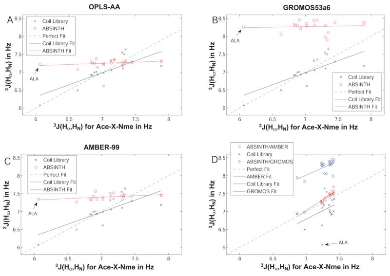
NMR ³J(H_αN_H) coupling constants obtained using ABSINTH's continuum solvation model coupled to standard force field parameters. Panel A shows the correlation between values measured by Avbelj et al. to the coil library as well as ABSINTH/OPLS-AA. Panels B and C show analogous plots for ABSINTH/GROMOS and ABSINTH/AMBER, respectively. Finally, Panel D shows a comparison of the values obtained with ABSINTH/OPLS-AA to the other two computational models as well as the coil library. Alanine is indicated in all plots as the most drastic outlier.

Panel A of Figure 4 shows that the values obtained for the OPLS-AA force field (circles) are insensitive to the type of sidechain, and that they are generally too large when compared to the direct measurements. Alanine is the most drastic outlier as indicated on the plot, but the agreement is generally poor. The values obtained from the coil library fits⁶⁸ show better agreement with experiment, although the slope of the correlation is less than unity for both comparisons implying larger similarity between simulated values and coil library fits compared to simulation and (direct) experiment. This suggests that the application of the Karplus equation to extract coupling constants inherently gives rise to some similarity, but might always deviate somewhat from direct measurements of the ³J(H_α,H_N).

The situation for the AMBER-99 force field is almost identical (Panel C), even though the values for the coupling constants are slightly larger, and hence further away from the measured values. Finally, the GROMOS53a6 force field (Panel B) is unable to generate reasonable coupling constants, because aliphatic hydrogen atoms - including the peptide α-hydrogen - are not actually steric interaction sites. This removes an important barrier for the ϕ-angle, normally separating the β- and polyproline II basins, and leads to vastly overestimated coupling constants. A comparison of these force fields to one another and to the coil library (Panel D) illustrates the extremely small range of coupling constants obtained using LJ parameters for standard force fields. This finding disagrees qualitatively with the predictions made based on coil libraries. We find excellent agreement between calculations based on parameters using the OPLS-AA and AMBER force fields, and this is noteworthy given the differences in the parameters.

Excluded volume interactions based on standard force field parameters (OPLS-AA, AMBER, and GROMOS) lead to severe restrictions in (ϕ,ψ)-space. This was inferred from visual inspection of Ramachandran maps (data not shown) and we concluded that LJ parameters from these standard force fields are not well suited for use with the ABSINTH model. This conclusion is justified based on the observations that: i) all coupling constants are too large, and ii) there is little to no sensitivity with sidechain type. Figure 5 shows that, we are able to remedy the deviation between the different parameter sets, irrespective of charge set used, by using a consistent LJ parameter set, which is detailed in Table II. These parameters are based on atomic radii in small molecule crystals,⁵⁰ and generic choices for the interaction strengths, intended to mimic values used in standard force fields.^1-3 As is apparent, these parameters coupled to any of the three charge sets (Panels A, B, and C) provide better agreement and a much larger sensitivity with respect to residue type. Prominent outliers with respect to the experimental values are alanine, aspartic acid, and histidine. Similarly, outliers with respect to the coil library are alanine, threonine, and aspartic acid, which are indicated in Panel D. Panel D also shows that we observe extremely good agreement for coupling constant values using substantially different charge sets.

Figure 5.

NMR ³J(H_αN_H) coupling constants obtained using ABSINTH's continuum solvation model coupled to modified LJ parameters and standard partial charge sets. Panels A, B, and C show the comparison of experimental values to the coil library values as well as the simulated results for the OPLS-AA (A), the GROMOS (B), and the AMBER (C) charges, respectively. Panel D shows a comparison between the values obtained with OPLS-AA to the other computational as well as the coil library data. Drastic outliers are indicated on the plots.

Within the continuum solvation model adopted in ABSINTH, steric interactions dominate the preferences for the ϕ-angle. Therefore, we are able to remedy deviations in local steric preferences by using a different, consistent set of LJ parameters with all three charge-sets and the hallmark of these LJ parameters is the smaller values for hard sphere radii. The only consistent and drastic outlier is alanine, for which we currently have no convincing explanation. The extremely low coupling constant seen experimentally suggests dominant population of the polyproline II- and α-basins, much more so than for any other residue type. Such a strong preference is inconsistent with the broadness of distributions in ϕ/ψ-space we generally observe in our simulations. Most other outliers involve charged residues, for which there typically is more variation in experiments as well, such as a significant dependence on pH,⁷⁵ which is difficult to represent in our continuum model. We also simulated capped pentapeptides with the sequence construct (Gly)₂-Xaa-(Gly)₂, for which there are experimental data under denaturing conditions.⁷⁶ Coupling constants are known to be insensitive to the presence of denaturant,⁷⁶ and hence we simulated these pentapeptides using the ABSINTH continuum solvation model. The calculated coupling constants obtained for residue Xaa in the context of flanking glycine residues are similar to those obtained for dipeptides (data not shown). This corroborates our conclusion that the LJ parameters are crucial for determining short-range structural preferences, which contribute to the measured values for vicinal coupling constants.

One could argue that the above result is due to the general absence of torsional parameters in ABSINTH, although there are exceptions as described in the Methods section. These parameters describe barriers and staggered conformations for rotations about bonds within polypeptides and one might question the validity of their omission. It has been noted that improvements in torsional parameters are crucial for quantitatively accurate descriptions of conformational equilibria for polypeptides.⁷⁷ To test our approach, we calculated conformational populations for alanine dipeptide and compared our results to those obtained by Hu et al..⁷⁸ These authors analyzed conformational equilibria for glycine and alanine dipeptides using a hybrid quantum mechanics / molecular mechanics (QM/MM) approach. They modeled intra-peptide interactions using the self-consistent charge density functional tight binding (SCCDFTB) method, whereas peptide-solvent and solvent-solvent interactions were described using standard molecular mechanics models. They compared their results to those obtained using a range of molecular mechanics force fields with explicit solvent. None of these agreed with the conformational distributions calculated using the QM/MM approach. They also noted that conformational distributions calculated with different molecular mechanics force fields did not agree with each other.

Table V shows conformational populations for alanine dipeptide, calculated using ABSINTH, and compared to those obtained by Hu et al. from their QM/MM calculations as well as their molecular mechanics calculations using different force fields. Hu et al. reported two sets of QM/MM data that were consistent with each other. The two calculations differed in the choice of LJ parameters used to describe the peptide for modeling peptide-solvent interactions. The QM/MM calculations did not include any empirical torsional potentials because all intra-peptide interactions were described using quantum mechanics. The results shown in Table V are very encouraging for our approach. When we compare the statistics for specific conformational intervals, it becomes clear that the results obtained using the ABSINTH force field show the best agreement with the QM/MM data. This point is also emphasized when we compare pairwise root mean square deviations between data obtained using different force fields and those obtained using QM/MM. Hu et al. also showed that their QM/MM data (and by extension the ABSINTH data) are in good agreement with statistics obtained from the distributions of ϕ and ψ angles in the protein data bank.⁷⁹

Table V.

Comparative analysis of conformational statistics for alanine dipeptide

	SCCDFTB amber 1	SCCDFTB Charmm221	amber1	charmm21	cedar1	gromos1	oplsaa1	oplsaa/l2	absinth3
beta	0.48	0.48	0.16	0.50	0.71	0.82	0.86	0.69	0.50
pass	0.16	0.14	0.00	0.00	0.00	0.00	0.00	0.06	0.09
alpha R	0.27	0.33	0.84	0.50	0.22	0.13	0.14	0.25	0.39
alpha L	0.07	0.03	0.00	0.00	0.05	0.04	0.00	0.00	0.01
state 4	0.01	0.01	0.00	0.00	0.02	0.01	0.00	0.00	0.01
RMSDI4	0.00	0.08	0.68	0.29	0.29	0.40	0.44	0.24	0.15
MaxDI5	0.00	0.06	0.57	0.23	0.23	0.34	0.38	0.21	0.12
RMSDII6	0.08	0.00	0.62	0.22	0.29	0.42	0.45	0.24	0.08
MaxDII7	0.06	0.00	0.51	0.17	0.23	0.34	0.38	0.21	0.06

¹Data for conformational statistics shown in columns 2-8 are taken from Tables I and II in the work of Hu et al..⁷⁸

²Values for conformational statistics were computed using molecular dynamics simulations. In these simulations, we used parameters from the OPLS-AA/L force field for the peptide and the TIP3P model for water molecules. The simulations were carried out with a single alanine dipeptide in a cubic box of side 25Å. The Berendsen thermostat (T=298K; coupling constant 0.1ps) and manostat (P=1bar; coupling constant, 1ps) were used to simulate the peptide in water in an isothermal-isobaric ensemble. The SETTLE algorithm was used to constrain bond lengths and bond angles for the water molecules, whereas the LINCS method was used to constrain all bond lengths in the peptide. A time step of 2.0fs was used and the equations of motion were integrated using the leap frog method as implemented in the GROMACS package. A 10Å spherical cutoff was used for both van der Waals and electrostatic interactions. Neighbor lists were updated once every five time steps and a reaction field with a bulk dielectric constant of 80 was used as a method to introduce corrections due to long-range electrostatic interactions. Data shown in the table are averages over 40 independent simulations, each of length 30ns.

³Values for conformational statistics were obtained using Metropolis Monte Carlo simulations. Details of the move sets used are shown in Table III.

⁴RMSD_I is the root-mean-square deviation between statistics shown in columns 2-10 (for the five conformational states) and the statistics shown in column 2 (SCCDFTB – amber).

⁵MAXD_I is the unsigned maximal deviation between statistics shown in columns 2-10 and the statistics shown in column 2 (SCCDFTB-amber).

⁶RMSD_II is the root-mean-square deviation between statistics shown in columns 2-10 (for the five conformational states) and the statistics shown in column 3 (SCCDFTB – charmm22).

⁷MAXD_II is the unsigned maximal deviation between statistics shown in columns 2-10 and the statistics shown in column 3 (SCCDFTB-charmm22).

The good agreement between QM/MM data and ABSINTH is very important because it suggests that the description of backbone conformational equilibria using ABSINTH is reasonable. The energy landscape obtained using QM/MM and ABSINTH for alanine dipeptide is in general flatter than what one obtains with the other force fields. It appears that the combination of LJ parameters and stiff torsional potentials in molecular mechanics force fields makes them too restrictive. This in turn might pose challenges for accurate modeling of conformational heterogeneity in IDPs because of significant pre-organization at the level of an individual residue. Given our interest in IDPs, as opposed to structure prediction, we propose that the ABSINTH approach might be a more reasonable alternative for simulating conformational heterogeneity that is characteristic of IDPs.

Thermal Unfolding of two Small Proteins

The 56-residue, B1 domain of streptococcal protein G is stable as an isolated construct and characterized by a well-defined α/β-fold and unusually high thermal stability. Its structure has been determined by NMR,⁸⁰ and the maximum melting temperature was found to be 87°C at a pH of 5.4.⁸¹ The exact melting temperature is strongly pH- and salt-dependent, with the stability expected to be significantly reduced at neutral pH based on a recent, systematic study on a structure-preserving mutant.⁸² The B1 domain has been studied extensively by computational methods as well.^83-85 Its α/β-fold, its initial characterization as a prototypical two-state folder, and its outstanding stability suggest that this domain is a useful test case for testing new models.

Ideally, the reversible folding of the B1 domain would be demonstrated by simulating the system from two different initial conditions (randomized vs. folded) over a wide range of temperatures. However, the entire domain folds on the ms-timescale, which is a regime that remains inaccessible to unbiased simulation techniques. Here, we show the results of MC simulations of the thermal unfolding of the B1 domain when starting from the folded structure (PDB: 1GB1). At low simulation temperatures, we expect the fold to remain stable, while at high temperatures, we expect full denaturation. The unfolding transition is known to be cooperative, another feature expected to be prominent in plots of folding measures against temperature. A study of thermal unfolding allows us to test two aspects of our model: First, we can assess if the folded species is a stable minimum for a given Hamiltonian. Second, we assess if the protein shows a cooperative transition between folded and unfolded states, in accord with experimental observations, and irrespective of the measure used to assess conformational stability. The second point is rarely addressed in simulation studies, since the primary interest often lies in the folded species. To describe phenomena such as folding, assembly, or disorder, however, it is crucial that the folded state is not over-stabilized.

Figure 6 shows three different folding measures for the B1 domain of protein G as a function of temperature, the first two of which are based on the root mean square deviation (RMSD) from the PDB structure after superposition, using different subsets of the protein. The third is the radius of gyration (R_g) of the molecule, a quantity used to describe its overall size, i.e., to monitor chain collapse / swelling. Both RMSD measures probe secondary and tertiary structure simultaneously. The thermal stability of the B1 domain has mostly been studied using differential scanning calorimetry and circular dichroism (CD) measurements, which have been shown to agree well in general.^81,82 The overall RMSD hence seems like a good candidate to unite the local and global features measured experimentally. Conversely, the R_g measure can only probe overall size and is shown to illustrate the polymeric behavior for this system.

Figure 6.

Unfolding measures for the B1 domain of protein G as a function of simulation temperature. Panel A shows two raw values for the RMSD to the PDB structure, i) for all heavy backbone atoms excluding the terminal residues; and ii) for just the heavy backbone atoms in the helical portion of the protein, along with the radius of gyration. The RMSD is based on structural alignments using only the corresponding residues as alignment criteria. Panel B shows values for all three measures normalized to their end points at 260K (0.0, fully folded) as well as 440K (1.0, fully unfolded). Error bars are obtained through block averaging, using a block size of 5×10⁵ MC steps.

As can be seen in Figure 6, all three measures report a cooperative and well-defined unfolding transition with well-defined baselines below 320K and above 380K. Interestingly, when normalized (Panel B) the two RMSD curves coincide almost perfectly indicating that the overall α/β-fold unfolds cooperatively rather than exhibiting disparate stability of the helical and β-sheet parts of the structure. Conversely, the R_g transition is shifted to slightly higher temperatures indicating that secondary structure melts out partially while the chain remains collapsed. Overall, however, swelling and unfolding are roughly concomitant. This observation, agrees with the apparent two-state folding behavior reported for this protein.^80,82 More importantly, the melting temperature in the model can be estimated to be around 340K (65-70°C), which is in good agreement with experiment when realizing that the cited 87°C^81,82 are obtained under conditions of maximum stability. The value also coincides well with the number given at low salt and neutral pH for the aforementioned mutant.⁸²

To further corroborate that folded proteins are stable minima and show reasonable temperature dependence we chose to study the engrailed homeodomain from Drosophila whose structure was solved to 2.1Å resolution by X-ray crystallography (PDB: 1ENH).⁸⁶ It is a three-helix bundle protein which undergoes thermal melting with a midpoint of about 45°C as monitored by CD^86,87. It serves as a good, complementary test case for the following reasons. First, it is among the fastest folders known to date,⁸⁸ which has enabled computer simulations to study the unfolding of this protein directly using MD in explicit solvent on a realistic timescale.^87,88 Second, it has been described as a difficult and hence a good test case for continuum solvation models.⁸⁹

Panel A of Figure 7 shows four different unfolding measures, which are all based on the RMSD from the PDB structure. If all the proteins heavy backbone atoms are aligned and the RMSD is computed, one obtains a melting curve with a very well-defined upper baseline, but a relatively high RMSD of about 3.5Å at low temperature, which continuously grows with increasing temperature. In contrast, if one uses the three helices independently to do the alignment and RMSD computation, helices A and B yield highly cooperative and well-defined melting transitions with a mid-point of about 330K, while helix C yields a more gradual transition resembling that of the whole protein, but shifted to slightly higher temperatures. In Panel B of Figure 7 all four unfolding measures are presented in normalized fashion assuming the baseline at low temperature is reasonably flat. As can be seen all measures taken together report on a broad transition region of 300-350K in agreement with experimental data.

Figure 7.

Unfolding measures for the engrailed homeodomain as a function of simulation temperature. Panel A shows four raw values for the RMSD to the PDB structure, which are based on all heavy backbone atoms excluding terminal residues as well as based on the heavy backbone atoms for the three helices individually. Using the PDB-numbering (1ENH) the helices were defined as residues 11 to 25 (A), residues 29 to 41 (B), as well as residues 43 to 57 (C). Likewise to Figure 6, the RMSD is based on structural alignments using only the corresponding residues as alignment criteria. Panel B shows values for the four measures normalized to their end points at 260K (0.0, fully folded) as well as 440K (1.0, fully unfolded). Error bars are obtained through block averaging, using a block size of 5×10⁵ MC steps.

We can interpret the data as follows. Unlike for the B1 domain of protein G, the tertiary contacts for the engrailed homeodomain are weak and have substantial residual entropy even at low temperatures. In other words, the relative arrangement of the three helices is not very tightly constrained. With increasing temperatures, tertiary contacts are lost completely, but alternative collapsed states with intact helices are visited transiently. This leads to intermediate values for the total RMSD and to large error bars in the transition region. Finally, at high temperature the chain expands fully, and the helices become unstable and melt. This picture obtained from the simulations is consistent with the conclusion from both experiments and computation that the folding of the engrailed homeodomain can be explained using the limiting diffusion-collision model,^88,90 in which pre-formed secondary structure elements “dock” to result in the folded tertiary structure. It is also consistent with the view that the system seems to be much less of a two-state system compared to the B1 domain of protein G and that helix-rich intermediates are populated along the folding/unfolding pathway.⁸⁸ Finally, our results somewhat contradict previous simulation work⁸⁷ in that we do not find the helices to be significantly populated at high temperatures. It should be noted, however, that the RMSD measure employed here fails to report on small, but significant populations of the helical state which we certainly observe for helices A and C, but not for helix B (data not shown), which is in agreement with the literature.⁸⁷

Regarding the reasonable agreement of T_m-values we find with the experimental literature, it must be pointed out that it is well known that simulation temperatures do not correspond to actual temperatures, because the phase behavior of the solvent is not captured by the continuum. In fact, the proper way to realize temperature dependence in ABSINTH would be to capture the thermal behavior of all the underlying parameters, including the reference free energies of solvation (decomposed into entropies and enthalpies), the continuum dielectric, and of course all atomistic parameters. The point here is not to provide quantitative agreement between melting temperatures, but to show that the model does not drastically over-stabilize the folded state.

Reversible folding / unfolding of the α-helical FS-peptide

The 21-residue FS-peptide (Acetyl-A₅[AAARA]₃-N-Methylamide) is a member of a class of extremely simple polypeptide systems, which undergo a folding transition in aqueous solution. Its melting temperature is estimated to be ca. 305K, i.e., the folded form is expected to be substantially populated at room temperature.^91-93 The α-helical nature of these peptides in the folded form has been established primarily through CD measurements and other spectroscopic techniques.

The FS-peptide is simple and allows us to simulate reversible folding / unfolding transitions as a function of temperature. Additionally, there have been several computational studies on the FS-peptide.^58,70,71 These studies show that the helical form is over-stabilized in simulations with standard force fields, and that ad hoc modifications such as the scaling of short-range interactions and the modulation of torsional potentials improve agreement with experimental data.^58,70 It is worth reiterating that the ABSINTH model does not employ ad hoc scaling parameters, nor does it include torsional potentials.

In Figure 8, we present the results from 20 independent simulations. For each of the ten temperature values there is both an unfolding simulation starting from the canonical α-helix and a folding simulation starting from a random, extended conformation. Panel A in Figure 8 shows the fractional α-helical content computed according to LR theory. A distinct and cooperative transition is found for both sets of temperature-dependent simulations. We observe virtually no hysteresis between the unfolding and refolding arms indicating that sampling is exhaustive. From the transition region, the melting temperature can be seen to be ∼330K, which is higher than the value of ∼305K obtained from experimental studies. However, as Table VI shows, the disagreement is smaller vis-à-vis previous computational studies using variants of the AMBER force field with either explicit solvent or a GB/SA continuum solvent description.⁷⁰ Panels B and C show how <N_h> and <N_s> vary as a function of temperature (see Equation 11). The data indicate that the dominant species at low temperatures is a single, straight α-helix, an observation confirmed by visual inspection of the trajectories (data not shown). The data around 300K are very similar to observations made by Nymeyer and Garcia (see Figures 1 and 2 in their work⁷⁰) using their modified version of AMBER in either explicit or implicit solvent.

Figure 8.

The temperature-dependence of the fractional helical content (Panel A), the mean number of helical hydrogen bonds (Panel B), and the mean number of helical segments of at least two residues in length (Panel C) in the FS-peptide. The folding and unfolding simulations are shown as solid and dashed lines, respectively. The dotted line in Panel A indicates a fractional helicity of 50%, which is used to roughly estimate the melting temperature.

Table VI.

Comparative analysis of parameters of the helix-coil transition for the FS-peptide.^*

Method	Tm in K	v (T in K)	w
Experiment	∼305	0.036 (273)	∼1.3
AMBER-94	393 / -	0.27 (300) / 0.36 (305)	2.12 / 1.67
AMBER-GS	342 / -	0.13 (300) / 0.70 (305)	1.67 / 3.70
AMBER-94 / GB/SA	380	0.79 (300)	2.20
AMBER-GS / GB/SA	431	1.57 (300)	4.03
AMBER-99	-	0.06 (305)	0.70
AMBER-99ϕ	-	0.26 (305)	1.26
AMBER-94 -SQ	-	0.28 (305)	1.28
ABSINTH	∼330	∼0.5 (300)	∼1.9

^*AMBER-94 is the full Cornell et al. force field¹, while AMBER-GS is the modification introduced by Garcia and Sanbonmatsu.¹²⁵ AMBER-99¹²⁶ is a more recent version known for its heliophobic nature, while AMBER-99ϕ is the correction introduced by Sorin and Pande.⁷¹ Finally, AMBER-94–SQ is a further modification introduced by Sorin and Pande shown to illustrate their more extensive study on the impact of non-covalent term scaling.⁵⁸ The second column shows the melting temperatures in K, the third and fourth columns the LR parameters at 300K or 305K, respectively. The are two different datasets shown for AMBER-94 and AMBER-GS, which come from Garcia's⁷⁰ and Pande's⁷¹ groups, respectively.

Figure 9 shows the LR nucleation and propagation parameters as a function of temperature in Panels A and B. These quantities have been estimated as outlined in the Methods section and describe the propensities to populate the α-helical basin in the absence of hydrogen bond stabilization, and to extend existing helix nuclei through hydrogen bond-stabilized growth. Panel A shows that w follows the trend for the overall helicity, and that it decreases from values around 2.8 to values around 0.45 throughout the temperature range studied here. Panel B shows that v is temperature-dependent as well, decreasing from values around 0.75 to values around 0.15. Just as we observed for the various measures of helicity in Figure 8, the hysteresis between unfolding and refolding arms is minimal indicating very well-converged data. Table VI shows that the estimates obtained using ABSINTH are generally comparable to values obtained with other force fields. The work of Nymeyer and Garcia⁷⁰ makes it clear that even though v and w might show better agreement with experiment, melting temperatures may be overestimated. Furthermore, the experimentally determined temperature-dependence of w⁹⁴ is crudely shown as a thick dashed line in Panel A of Figure 9. Obviously, ABSINTH slightly overestimates the propagation parameter, but it does seem to provide a reasonable representation of the slope. If anything, the latter seems to be slightly overestimated, which stands in contrast to the AMBER-based models deemed most reasonable, for which the slope seems to be underestimated.⁷¹ The most relevant comparison in Table VI is between the simulations using the GB/SA model and ABSINTH, and for this specific system, the latter shows better agreement with experiments than the former, and this holds for all the measures used to quantify helix-coil transitions as shown in Table VI.

Figure 9.

The temperature-dependence of the Lifson-Roig (LR) nucleation (Panel A) and propagation (Panel B) parameters shown analogously to Figure 8. Dotted lines indicate a temperature of 300K. The thick dashed line in Panel A is the experimentally determined temperature dependence of the propagation parameter. Panel C shows predictions for the mean, fractional number of helical hydrogen bonds (lower set of curves) and for the mean number of helical segments (upper set of curves) from LR theory as a function of the nucleation parameter. A family of curves for values of w = 1.27, 1.42, 1.57, 1.72, 1.87, 2.02, 2.17 is shown in either case. Increasing values of w are shown as lighter-colored graphs and dashed and solid lines alternate for better clarity.

Two additional points need to be made. As has been noted in the literature, v is generally overestimated by roughly an order of magnitude in simulations. We suggest that this is partly due to the method employed for analyzing simulation data. In experiments, v is obtained through fits to kinetic data on helix nucleation,^95,96 while computationally it is obtained through fits to the equilibrium population of helix segments. Panel C in Figure 9 shows predictions from LR theory as a function of v. Clearly, for large enough values of w, high helicity coupled to an average number of helical segments significantly larger than unity (as is usually observed) is only possible if v is substantially larger than the experimentally determined value of 0.036. Even at high temperatures, when entropy dominates, it is impossible to observe very low values for v given the way we compute this parameter from simulation data. This point will be addressed in detail elsewhere. Finally, Table VI allows one to make comparisons between the AMBER and OPLS-AA charge sets. It should be noted that the latter were used for the ABSINTH calculations shown here. Gnanakaran and Garcia⁹⁷ have observed sharper transitions in their study of a related peptide Ala₂₁ using explicit solvent and the OPLS-AA/L force field⁷⁷, suggesting that the lack of cooperativity in AMBER might be due to the charge set employed.

The Reversible “Folding” of a β-Hairpin Peptide

For peptides engineered to fold into a β-hairpin, there often is no well-defined transition between the folded and unfolded ensembles. The thermal denaturation of these systems usually shows a broad transition with ill-defined baselines and little cooperativity.^73,98,99 We can summarize the differences with respect to α-helical peptides as follows:

• The folding of α-helical systems is backbone-driven. This is apparent from the fact that low-complexity sequences such as the FS-peptide do in fact fold and that the simplest chiral residue (alanine) is the one with the largest helix propensity.^100,101 Conversely, the folding of β-hairpins or three-stranded β-sheets is sidechain-driven. This point is made by the fact that design attempts succeed by focusing on optimizing the turn sequence and the sidechain registry.^{73,98,102,103} In other words, the chiral peptide backbone of short peptides in aqueous solution shows an intrinsic propensity to populate α-helical, but not β-rich conformations. This is illustrated indirectly by the prevalence of ordered, β-rich structures in environments which become less and less aqueous such as protein aggregates¹⁰⁴ or organic solvent mixtures.¹⁰⁵

• The folding of α-helical systems is well-described by simple models (see above), whereas that of short β-sheet peptides is distinctively heterogeneous and highly sensitive to the experimental probe employed.⁹⁹

• The folded ensemble for α-helical systems is characterized by residual entropy in fraying ends, bending, and possible kinks, but always remains well-described by local backbone propensities and the i to i+4 hydrogen bond registry.⁷² Conversely, the folded ensemble for most β-sheet peptides is almost exclusively constrained by non-local effects such as the arrangement of sidechains coming from opposite strands. Experimentally this type of ordering relates to the fluorescence of aromatic residues^73,99 or NMR order parameters such as NOEs.^102,106

• The kinetics for helix formation are at least an order of magnitude faster than those for hairpin formation.¹⁰⁷ Hence, systems of the latter type pose a much stiffer challenge for computational efforts trying to demonstrate reversible folding.

Most of the simulation studies carried out on β-hairpin peptides have focused on a fragment of the B1 domain of protein G, more precisely the C-terminal hairpin, as it was shown to exhibit features resembling the “native” hairpin experimentally.¹⁰⁶ However, the order parameters chosen in simulation work usually do not relate to experimental probes directly, and hence the relevance of such results for the goal of calibrating force fields is questionable. Moreover, it was recently shown that the NMR data are in fact much more consistent with highly disordered simulation ensembles involving large populations of non-native like structures than with predominantly folded ensembles.¹⁰⁸

The preceding discussion leads us to choose the so-called tryptophan zippers as our model system. These are very short peptides with two tryptophan pairs on either side which “zip” together to stabilize the β-hairpin conformation.⁷³ NMR structures could be obtained using distance as well as dihedral restraints. From a simulation standpoint, the system has been studied most extensively using continuum solvation models of the GB/SA flavor.^{74,99,109,110} Even in a continuum solvent sampling is surprisingly difficult given the small size of these peptides. The system was shown to exhibit heterogeneity both in terms of the kinetics of its thermal unfolding behavior in aqueous solution⁹⁹ and in terms of its simulated conformational equilibrium at temperatures, for which experimental data are interpreted to indicate dominant population of the folded basin.¹⁰⁹

Here, we study “trpzip1” (pdb code: 1LE0),⁷³ which has the lowest melting temperature among the 12-residue designs, but seems to show the cleanest transition between predominantly folded and predominantly unfolded ensembles. Even for this system, however, the experimental data are interpreted to imply that the fraction of folded molecules decreases almost linearly from 0.8 to 0.1 over the wide temperature range of 300 to 360K. Moreover, the maximum folded population is never expected to exceed 0.8, hence indicating substantial residual disorder even in the low-temperature regime. Figure 10 shows the temperature dependence of various order parameters for simulations starting from either random extended conformations (folding simulation) or from the NMR structure, more precisely the first model (unfolding simulation). In general, both sets of simulations agree very well with one another. At 300K, however, discrepancies start to arise, and we could not generate hysteresis-free data for temperatures below 300K. This agrees with previous studies which had to use substantially elevated temperatures to simulate tryptophan zippers.^109,111

Figure 10.

The temperature dependence of various order parameters characterizing the simulated ensembles of the tryptophan zipper “trpzip1”. Sets of folding and unfolding simulations are shown as solid and dashed lines, respectively. Panel A shows the heavy backbone atom RMSD to the PDB structure (Model 1 in 1LE0) excluding the N-terminal serine and the C-terminal amide cap. Panel B shows the radius of gyration of the sidechains of the four tryptophan residues. Panel C shows the mean strand-to-strand distance for the perfect hairpin, whereas the order parameter L as defined by Snow et al.⁷⁴ is shown in Panel D.

Panel A of Figure 10 shows the mean RMSD, which decreases with decreasing temperature, but only reaches a value of 3.5 at 300K. Panel B shows the radius of gyration of the hydrophobic cluster driving hairpin formation, i.e., the sidechains of the four tryptophan residues. This is an order parameter typically used for β-hairpin systems,^112,113 since it addresses the driving force for folding directly. For the tryptophane zippers, however, the NMR structures do not show a true hydrophobic cluster, but instead show the indole rings to be in an edge-to-face arrangement on one face of the hairpin with substantial solvent-accessibility and no stacking or hydrogen bonds. Guvench and Brooks¹¹⁴ argue that this unusual structure arises due to the electrostatic multipoles in the non-polar parts of the indole rings. The NMR ensemble has a resultant value for the R_g of the hydrophobic cluster of 6.4Å, which is actually larger than what we observe at 300K. Panel C shows the average distance strand-to-strand distance. The behavior is similar to that seen for the backbone RMSD in that the value for the NMR ensemble (4.8Å) is approached with decreasing temperature, but that even at 300K the deviation is quite substantial. Similarly, the order parameter L as defined by Snow and co-workers⁷⁴ takes into account native hydrogen bond distances as well as sidechain-sidechain distances for the trypophan pairs found in contact experimentally. Panel D shows that L behaves similarly to both the RMSD and the mean strand-to-strand distance with the NMR ensemble yielding an average L of 27.9Å.

In summary, these results indicate that the ABSINTH Hamiltonian samples predominantly disordered conformations which emphasize the driving force for the collapse of the hairpin, but fail to predominantly populate the specific structure determined by NMR. In an average sense, a broad basin of structures with native-like features becomes more and more populated with decreasing temperature, which is in accordance with the experimental data on thermal melting, but contradicts the folding estimates deduced from such data.⁷³ Yang et al.⁹⁹ have shown for “trpzip2” that by various spectroscopic probes multiple melting transitions can be identified, none of which can be interpreted to uniquely report on the loss of the specific NMR structure as the order parameters in Panels A, C, and D of Figure 10 do.

In order to show the differences and similarities between our results and those of other simulation studies we computed two-dimensional potentials of mean force (PMFs) in various combinations of order parameters. Figure 11 shows plots analogous to Figure 3a in the work of Snow et al.⁷⁴ for the folding (Panel A) and unfolding simulations (Panel D) at 300K, respectively. In these PMFs of order parameter L vs. the backbone RMSD, the native state would be located in the lower left corner. Clearly, the precise NMR structure is not a relevant part of the free energy landscape. Instead, structures with native-like low L values or low backbone RMSDs are observed independently of one another. This means for example that misfolded hairpins with non-native tryptophan arrangements are observed. In Panel B we can identify such a misfolded hairpin basin for low values of both the strand-to-strand distance and L, which was not observed to the same extent in the unfolding simulation (Panel E). Panels C and F show PMFs as a function of the number of strand-to-strand hydrogen bonds vs. R_g of the hydrophobic cluster, and illustrate this point more clearly. For the folding simulation we found a weak, but distinct basin of conformations with substantial hydrogen bonding. In both cases, however, the vast majority of conformations has little to no strand-to-strand hydrogen bonds. It is crucial to point out that in the work of Snow et al. the PMFs are created by analysis of a vast number of independent simulations starting from extended states. While they discard a sufficiently long equilibration phase (100ns, which is several times the collapse time), the free energy surfaces are not equilibrated, and the unfolded state is overrepresented.

Figure 11.

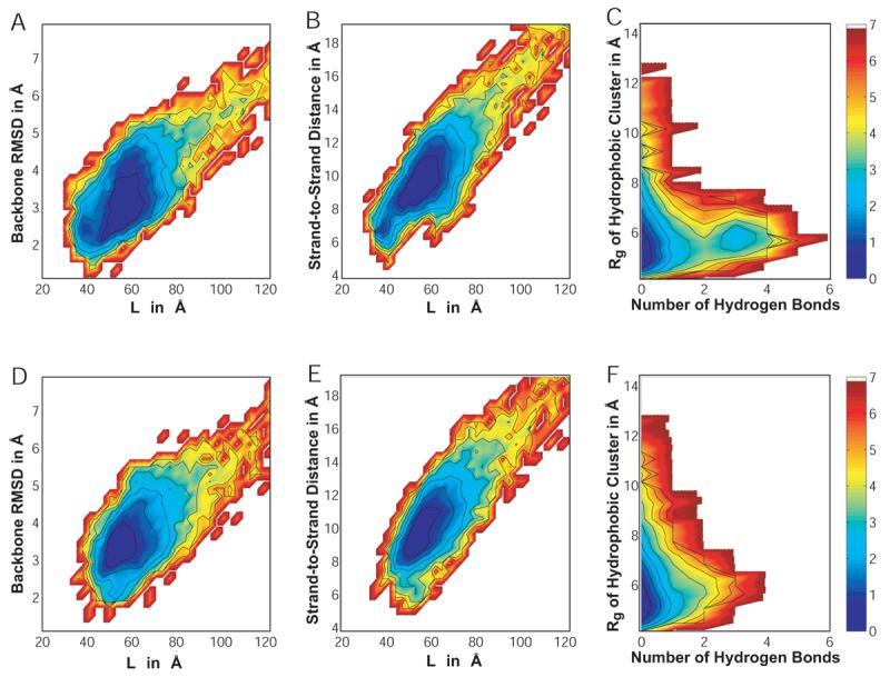
Various two-dimensional potentials of mean force for combinations of order parameters (see Methods and Figure 10). The data are obtained at 300K and are shown for the folding simulation in Panels A, B, and C, and for the unfolding simulation in Panels D, E, and F.

This leads to the following major conclusions for “trpzip1”:

• The native basin as defined by a specific NMR structure is not a stable conformation for the ABSINTH Hamiltonian. It is noteworthy that Snow et al. show that the OPLS-UA force field coupled to the GB/SA continuum solvent is equally unable to stabilize the native basin, and that – unlike common practice – no 14-scaling was employed in any of their OPLS-AA/GB results. This is an important modification of the force field, because the underlying energy landscape may depend astutely on this choice,⁵⁸ in particular in a continuum solvent as discussed in the Methods section.

• A broad basin of states with native-like topology is populated readily and increasingly so with decreasing temperature. This finding suggests that the ABSINTH model can be used to reliably identify native-like basins albeit in a coarse-grained manner.

At this point, we wish to re-emphasize that ABSINTH is not designed as a structure prediction tool. For the applications of interest, it appears more beneficial to underpredict rather than to overpredict the specific structural preferences of polypeptides. While we are actively invested in understanding what components of our model lead to the observed discrepancies for “trpzip1”, we also wish to point out that this result does not imply a general problem of the model in dealing with β-structures. This assertion is supported by our results for the B1 domain of protein G, for which we observe cooperative unfolding in agreement with experimental data indicating that within the context of the full-length protein the hairpin is not destabilized. Therefore we do not pursue tuning of ABSINTH to generate stable hairpins given that the experimental data suggest that such an approach would be unjustified and that the ensembles for such short peptides are indeed heterogeneous.¹⁰⁸

Polymeric behavior of polyglutamine

We have shown, both experimentally⁸ and computationally^10,115, that homopolypeptides composed predominantly of glutamine exhibit a strong preference for collapsed states in aqueous solution. They are intrinsically disordered, and have no marked preference for canonical secondary structures. The latter point is supported by experimental results based on CD and NMR spectroscopy^116-118 as well as high-resolution computational studies, i.e., molecular dynamics (MD) simulations in explicit solvent.¹¹⁵ The collapsed nature of the ensemble can be established through a polymeric scaling law, i.e., the change in size of the molecules with chain lengths. For chains in a poor solvent, i.e., a solvent in which chain-chain contacts are preferred over chain-solvent contacts, collapsed states are preferred and the radius of gyration should scale with chain length N with a scaling exponent of ∼0.33:

$$\langle R_g\rangle =R_{\mathrm{o}}{N}^{\nu };\text{where}\nu =\frac{1}{3}$$ (12)

Here, 〈R_g〉 is the ensemble-averaged radius of gyration of an individual polypeptide chain, N is the chain length, ν is the actual scaling exponent, and R_o is a parameter related to the monomer size. By plotting 〈R_g〉 versus N in a double-logarithmic plot, one can obtain the scaling exponent through linear regression. In previous computational work,^10,115 we were unable to actually measure the scaling exponent due to the prohibitive cost of such simulations. Instead, we compared the polymeric behavior of Q₂₀ in water to two reference models, and established through alternate means that these chains form collapsed globules and that water is indeed a poor solvent even for such short glutamine-rich peptides.

Figure 12 shows the double-logarithmic plot of 〈R_g〉 versus N obtained using ABSINTH compared to the two reference states extracted from previous work.¹⁰ The preference for collapsed states is preserved in the continuum solvation model and this result agrees with both theory and experiment. Using the uncertainty in the data themselves, we used MC re-sampling of the raw data to obtain an error margin for the scaling exponent of 0.33 ≤ ν ≤ 0.45. Clearly, this is only consistent with poor solvent scaling, and not with good solvent scaling, which is observed in the excluded volume (EV) limit, as shown in Figure 12. Moreover, the Experimental results⁸ arrive at similar conclusions with regards to the scaling exponent.

Figure 12.

Scaling law for the peptide series Acetyl-(Gln)_N-N-Methylamide. The data obtained with ABSINTH's solvation model is compared to the data for two reference models used in previous work. Error bars on the data for ABSINTH indicate a crude estimate of the reliability of the R_g-values based on the standard deviation of the averages of four independent runs. The uncertainty in the fit parameters was estimated using 50000 independent samples of the data drawn from the estimated normal distributions for each chain length. Due to the crude determination of the parameters for the latter distributions, the numbers are not to be viewed as a rigorous, statistical error estimate.

However, the scaling exponent is not necessarily the best illustration of solvent quality, as small amounts of noise in the data can lead to substantial variability in its estimate. Figure 13 shows a more detailed comparison of 30 independent trajectories for Q₂₀ to the MD simulations we carried out for the same system¹⁰. Here, we plot the scaling of internal distances (see Equation 5 in our previous work¹⁰) using ABSINTH compared to the calculation in explicit solvent as published. Differences between the two sets of results are mostly statistically insignificant, suggesting that for intrinsically disordered polyglutamine, differences in conformational averaging between the implicit and explicit solvent calculations are negligible. Both curves also coincide with the globular reference state indicating that in both explicit and implicit models of solvation, water is in fact a poor solvent for these peptides. Furthermore, we analyzed contact maps (data not shown) and concluded that overall there seems to be little to no preference for any kind of consensus secondary structure, even though backbone segment statistics indicate that extended stretches of α-helix are encountered in a few of the simulations. The observed preference for disorder is in agreement with both experiment and the previous computational studies.

Figure 13.

The scaling of internal distances with sequence separation. The data shown are the novel results obtained with ABSINTH compared to published results obtained in explicit solvent as well as the two reference models¹⁰. Error bars are shown for the data in explicit solvent and in ABSINTH and are obtained by calculating the standard deviation of the final averages for each of the 60 and 30 trajectories used, respectively.

Discussion and Conclusions

In this manuscript, we have introduced a new continuum solvation model termed ABSINTH. The following paragraphs outline why we think it represents a worthy addition to the available continuum solvation models.

ABSINTH is promising

For the test systems analyzed in this manuscript, ABSINTH provides a reasonable description of the underlying physics. Most results are in general agreement with what is known from experiments with two notable exceptions, i) we find specific outliers in the analysis of NMR coupling constants, and ii) we find that the ABINTH Hamiltonian fails to predict the specific NMR structure for the tryptophan zipper “trpzip1”. For the latter, however, the results are not necessarily in fundamental disagreement with the published experimental data as a function of temperature. The test cases here probe the short-range steric preferences of short peptides, the general polymeric nature of Q₂₀, the thermal stability of two small proteins, and reversible folding of both an α-helical and a β-hairpin peptide. Therefore, we conclude that ABSINTH is suitable for simulating processes such as folding/unfolding and self-assembly with semi-quantitative accuracy. The principles underlying phenomena of biological interest are identical, and hence the physical model behind ABSINTH should always apply. We wish to reiterate, however, that ABSINTH was calibrated with a focus on disordered systems, and hence appears unsuitable as a protein structure prediction tool in its current incarnation.

ABSINTH shares a lot of similarities with the EEF1 model of Lazaridis and Karplus, which has been successfully applied in a variety of contexts^119-122. ABSINTH, however, has novel aspects, which include the protocol used to calculate the solvent-accessible volumes; the use of small molecule solutes as solvation groups; the description of partially solvated states; and the screening of Coulomb interactions based on the local solvation environment. The features listed above make ABSINTH a useful model for continuum solvation, which combines aspects of the EEF1 and GB models.

ABSINTH is tunable

It is worth noting that the continuum solvation model can be tuned to change the nature of the solvent. This can be accomplished by varying the solvation parameters r_w, τ_s, χ_s, τ_d, and χ_d. These parameters modulate properties of solvent by tuning the stability of and the cooperativity of transitions between differently solvated states. Similarly, broad changes can be introduced by swapping out parameter sets for the LJ parameters or partial charges as demonstrated in some of our results. In ongoing work, we are using the temperature-induced helix-coil transition as a case study to illustrate the tunability of the model. It is also possible to carry out simulations including co-solutes such as urea and/or explicit water molecules using the same underlying paradigm, as we have demonstrated for inorganic ions in this work. Finally, there is no fundamental barrier to replace water as the continuum solvent, as long as the reference free energies of solvation and bulk dielectric are known experimentally for the alternative solvent of interest.¹²¹

ABSINTH has potential for substantial improvement

All results shown in this manuscript were obtained using MC sampling. Obvious improvements include a switch to a stochastic dynamics approach or even hybrid methods. The treatment of ionic groups as part of the polypeptide and in the bulk provides room for improvement. The goal is to be able to seamlessly integrate the explicit representation of the polymers in aqueous solution with the explicit representations of mobile counterions, which semi-quantitatively capture experimentally observed properties. In addition, the impact of our modified model for short-range electrostatic interactions needs to be analyzed in detail. Possible corrections based on comparison to quantum-chemical data may be required. Finally, a detailed analysis of the model's sensitivity to all its parameters including the LJ and partial charge sets, and the solvation parameters r_w, τ_s, χ_s, τ_d and χ_d should be performed. For this analysis, a more well-defined set of calibration systems and a more systematic approach will likely be necessary pending the availability of resources for such an endeavor. These improvements are part of our current research directions and hence pursued actively.

Concluding Statement

The guiding principle for developing ABSINTH is that implicit solvent models should offer significant computational savings over models representing all solvent molecules explicitly, while not introducing qualitative errors into the description of the physics of solvation. As was pointed out in the Introduction, numerous approaches have been brought forth to fulfill the aforementioned principle. Given the varying successes of these models, we see the need for an alternative approach, which combines the strengths of existing methods. It is our hope that its computational efficiency, its tunability, and its promising agreement with experimental results make ABSINTH an attractive tool for other researchers to complement available computational methods.

Bibliography

- 1.Cornell WD, Cieplak P, Bayly CI, Gould IR, Merz KM, Ferguson DM, Spellmeyer DC, Fox T, Caldwell JW, Kollman PA. J Am Chem Soc. 1995;117(19):5179–5197. [Google Scholar]
- 2.Oostenbrink C, Villa A, Mark AE, Van Gunsteren WF. J Comput Chem. 2004;25(13):1656–1676. doi: 10.1002/jcc.20090. [DOI] [PubMed] [Google Scholar]
- 3.Jorgensen WL, Maxwell DS, TiradoRives J. J Am Chem Soc. 1996;118(45):11225–11236. [Google Scholar]
- 4.MacKerell AD, Bashford D, Bellott M, Dunbrack RL, Evanseck JD, Field MJ, Fischer S, Gao J, Guo H, Ha S, Joseph-McCarthy D, Kuchnir L, Kuczera K, Lau FTK, Mattos C, Michnick S, Ngo T, Nguyen DT, Prodhom B, Reiher WE, Roux B, Schlenkrich M, Smith JC, Stote R, Straub J, Watanabe M, Wiorkiewicz-Kuczera J, Yin D, Karplus M. J Phys Chem B. 1998;102(18):3586–3616. doi: 10.1021/jp973084f. [DOI] [PubMed] [Google Scholar]
- 5.van Gunsteren WF, Mark AE. Eur J Biochem. 1992;204(3):947–961. doi: 10.1111/j.1432-1033.1992.tb16716.x. [DOI] [PubMed] [Google Scholar]
- 6.Feig M, Brooks CL. Curr Opin Struct Biol. 2004;14(2):217–224. doi: 10.1016/j.sbi.2004.03.009. [DOI] [PubMed] [Google Scholar]
- 7.Uversky VN, Gillespie JR, Fink AL. Prot Struct Funct Gen. 2000;41(3):415–427. doi: 10.1002/1097-0134(20001115)41:3<415::aid-prot130>3.0.co;2-7. [DOI] [PubMed] [Google Scholar]
- 8.Crick SL, Jayaraman M, Frieden C, Wetzel R, Pappu RV. Proc Natl Acad Sci U S A. 2006;103(45):16764–16769. doi: 10.1073/pnas.0608175103. [DOI] [PMC free article] [PubMed] [Google Scholar]
- 9.Moglich A, Joder K, Kiefhaber T. Proc Natl Acad Sci U S A. 2006;103(33):12394–12399. doi: 10.1073/pnas.0604748103. [DOI] [PMC free article] [PubMed] [Google Scholar]
- 10.Vitalis A, Wang X, Pappu RV. Biophys J. 2007;93(6):1923–1937. doi: 10.1529/biophysj.107.110080. [DOI] [PMC free article] [PubMed] [Google Scholar]
- 11.Baker NA. Curr Opin Struct Biol. 2005;15(2):137–143. doi: 10.1016/j.sbi.2005.02.001. [DOI] [PubMed] [Google Scholar]
- 12.Baker NA, Sept D, Joseph S, Holst MJ, McCammon JA. Proc Natl Acad Sci U S A. 2001;98(18):10037–10041. doi: 10.1073/pnas.181342398. [DOI] [PMC free article] [PubMed] [Google Scholar]
- 13.Simonson T. Curr Opin Struct Biol. 2001;11(2):243–252. doi: 10.1016/s0959-440x(00)00197-4. [DOI] [PubMed] [Google Scholar]
- 14.Still WC, Tempczyk A, Hawley RC, Hendrickson T. J Am Chem Soc. 1990;112(16):6127–6129. [Google Scholar]
- 15.Onufriev A, Case DA, Bashford D. J Comput Chem. 2002;23(14):1297–1304. doi: 10.1002/jcc.10126. [DOI] [PubMed] [Google Scholar]
- 16.Grycuk T. J Chem Phys. 2003;119(9):4817–4826. [Google Scholar]
- 17.Ooi T, Oobatake M, Nemethy G, Scheraga HA. Proc Natl Acad Sci U S A. 1987;84(10):3086–3090. doi: 10.1073/pnas.84.10.3086. [DOI] [PMC free article] [PubMed] [Google Scholar]
- 18.Chandler D. Nature. 2005;437(7059):640–647. doi: 10.1038/nature04162. [DOI] [PubMed] [Google Scholar]
- 19.Pierotti RA. Chem Rev. 1976;76(6):717–726. [Google Scholar]
- 20.Huang DM, Chandler D. J Phys Chem B. 2002;106(8):2047–2053. [Google Scholar]
- 21.Wagoner JA, Baker NA. Proc Natl Acad Sci U S A. 2006;103(22):8331–8336. doi: 10.1073/pnas.0600118103. [DOI] [PMC free article] [PubMed] [Google Scholar]
- 22.Gallicchio E, Kubo MM, Levy RM. J Phys Chem B. 2000;104(26):6271–6285. [Google Scholar]
- 23.Gallicchio E, Levy RM. J Comput Chem. 2004;25(4):479–499. doi: 10.1002/jcc.10400. [DOI] [PubMed] [Google Scholar]
- 24.Feig M, Onufriev A, Lee MS, Im W, Case DA, Brooks CL. J Comput Chem. 2004;25(2):265–284. doi: 10.1002/jcc.10378. [DOI] [PubMed] [Google Scholar]
- 25.Warshel A, Papazyan A. Curr Opin Struct Biol. 1998;8(2):211–217. doi: 10.1016/s0959-440x(98)80041-9. [DOI] [PubMed] [Google Scholar]
- 26.Im WP, Lee MS, Brooks CL. J Comput Chem. 2003;24(14):1691–1702. doi: 10.1002/jcc.10321. [DOI] [PubMed] [Google Scholar]
- 27.Haberthur U, Majeux N, Werner P, Caflisch A. J Comput Chem. 2003;24(15):1936–1949. doi: 10.1002/jcc.10317. [DOI] [PubMed] [Google Scholar]
- 28.Ferrara P, Apostolakis J, Caflisch A. Prot Struct Funct Gen. 2002;46(1):24–33. doi: 10.1002/prot.10001. [DOI] [PubMed] [Google Scholar]
- 29.Lazaridis T, Karplus M. Prot Struct Funct Gen. 1999;35(2):133–152. doi: 10.1002/(sici)1097-0134(19990501)35:2<133::aid-prot1>3.0.co;2-n. [DOI] [PubMed] [Google Scholar]
- 30.Privalov PL, Makhatadze GI. J Mol Biol. 1993;232(2):660–679. doi: 10.1006/jmbi.1993.1417. [DOI] [PubMed] [Google Scholar]
- 31.Mallik B, Masunov A, Lazaridis T. J Comput Chem. 2002;23(11):1090–1099. doi: 10.1002/jcc.10104. [DOI] [PubMed] [Google Scholar]
- 32.Patriciu A, Chirikjian GS, Pappu RV. J Chem Phys. 2004;121(24):12708–12720. doi: 10.1063/1.1821492. [DOI] [PubMed] [Google Scholar]
- 33.Perchak D, Skolnick J, Yaris R. Macromolecules. 1985;18(3):519–525. [Google Scholar]
- 34.Karplus M, Kushick JN. Macromolecules. 1981;14(2):325–332. [Google Scholar]
- 35.Echenique P, Calvo I, Alonso JL. J Comput Chem. 2006;27(14):1733–1747. doi: 10.1002/jcc.20467. [DOI] [PubMed] [Google Scholar]
- 36.Ben-Naim A, Marcus Y. J Chem Phys. 1984;81(4):2016–2027. [Google Scholar]
- 37.Levy RM, Zhang LY, Gallicchio E, Felts AK. J Am Chem Soc. 2003;125(31):9523–9530. doi: 10.1021/ja029833a. [DOI] [PubMed] [Google Scholar]
- 38.Alder BJ, Pollock EL. Annu Rev Phys Chem. 1981;32:311–329. [Google Scholar]
- 39.Paulaitis ME, Pratt LR. Unfolded Proteins. 2002:283–310. [Google Scholar]
- 40.Castleman AW, Keesee RG. Chem Rev. 1986;86(3):589–618. [Google Scholar]
- 41.Jorgensen WL, Gao J, Ravimohan C. J Phys Chem. 1985;89(16):3470–3473. [Google Scholar]
- 42.Swanson JMJ, Mongan J, McCammon JA. J Phys Chem B. 2005;109(31):14769–14772. doi: 10.1021/jp052883s. [DOI] [PubMed] [Google Scholar]
- 43.Lee MS, Olson MA. J Phys Chem B. 2005;109(11):5223–5236. doi: 10.1021/jp046377z. [DOI] [PubMed] [Google Scholar]
- 44.Im W, Beglov D, Roux B. Comput Phys Commun. 1998;111(13):59–75. [Google Scholar]
- 45.Onufriev A, Bashford D, Case DA. J Phys Chem B. 2000;104(15):3712–3720. [Google Scholar]
- 46.Qiu D, Shenkin PS, Hollinger FP, Still WC. J Phys Chem A. 1997;101(16):3005–3014. [Google Scholar]
- 47.Schaefer M, Karplus M. J Phys Chem. 1996;100(5):1578–1599. [Google Scholar]
- 48.Hawkins GD, Cramer CJ, Truhlar DG. J Phys Chem. 1996;100(51):19824–19839. [Google Scholar]
- 49.Zhou RH, Friesner RA, Ghosh A, Rizzo RC, Jorgensen WL, Levy RM. J Phys Chem B. 2001;105(42):10388–10397. [Google Scholar]
- 50.Hopfinger AJ. Conformational Properties of Macromolecules. Academic Press; New York: 1973. [Google Scholar]
- 51.Tran HT, Wang XL, Pappu RV. Biochemistry. 2005;44(34):11369–11380. doi: 10.1021/bi050196l. [DOI] [PubMed] [Google Scholar]
- 52.Villa A, Mark AE. J Comput Chem. 2002;23(5):548–553. doi: 10.1002/jcc.10052. [DOI] [PubMed] [Google Scholar]
- 53.Chang J, Lenhoff AM, Sandler SI. J Phys Chem B. 2007;111(8):2098–2106. doi: 10.1021/jp0620163. [DOI] [PubMed] [Google Scholar]
- 54.Shirts MR, Pitera JW, Swope WC, Pande VS. J Chem Phys. 2003;119(11):5740–5761. [Google Scholar]
- 55.Shirts MR, Pande VS. J Chem Phys. 2005;122(13) doi: 10.1063/1.1877132. [DOI] [PubMed] [Google Scholar]
- 56.Udier-Blagovic M, De Tirado PM, Pearlman SA, Jorgensen WL. J Comput Chem. 2004;25(11):1322–1332. doi: 10.1002/jcc.20059. [DOI] [PubMed] [Google Scholar]
- 57.Mobley DL, Dumont E, Chodera JD, Dill KA. J Phys Chem B. 2007;111(9):2242–2254. doi: 10.1021/jp0667442. [DOI] [PubMed] [Google Scholar]
- 58.Sorin EJ, Pande VS. J Comput Chem. 2005;26(7):682–690. doi: 10.1002/jcc.20208. [DOI] [PubMed] [Google Scholar]
- 59.Fitzgerald JE, Jha AK, Sosnick TR, Freed KF. Biochemistry. 2007;46(3):669–682. doi: 10.1021/bi061575x. [DOI] [PubMed] [Google Scholar]
- 60.Vlachy V. Annu Rev Phys Chem. 1999;50:145–165. doi: 10.1146/annurev.physchem.50.1.145. [DOI] [PubMed] [Google Scholar]
- 61.Friedman HL. Annu Rev Phys Chem. 1981;32:179–204. [Google Scholar]
- 62.Vitalis A, Baker NA, McCammon JA. Mol Simul. 2004;30(1):45–61. [Google Scholar]
- 63.Pliego JR, Riveros JM. Phys Chem Chem Phys. 2002;4(9):1622–1627. [Google Scholar]
- 64.Marcus Y. J Chem Soc Farad Trans. 1991;87(18):2995–2999. [Google Scholar]
- 65.Kang YK, Nemethy G, Scheraga HA. J Phys Chem. 1987;91(15):4105–4109. [Google Scholar]
- 66.Engh RA, Huber R. Acta Crystallogr A. 1991;47:392–400. [Google Scholar]
- 67.Karplus M. J Chem Phys. 1959;30(1):11–15. [Google Scholar]
- 68.Avbelj F, Baldwin RL. Proc Natl Acad Sci U S A. 2003;100(10):5742–5747. doi: 10.1073/pnas.1031522100. [DOI] [PMC free article] [PubMed] [Google Scholar]
- 69.Lifson S, Roig A. J Chem Phys. 1961;34(6):1963–1974. [Google Scholar]
- 70.Nymeyer H, Garcia AE. Proc Natl Acad Sci U S A. 2003;100(24):13934–13939. doi: 10.1073/pnas.2232868100. [DOI] [PMC free article] [PubMed] [Google Scholar]
- 71.Sorin EJ, Pande VS. Biophys J. 2005;88(4):2472–2493. doi: 10.1529/biophysj.104.051938. [DOI] [PMC free article] [PubMed] [Google Scholar]
- 72.Hong Q, Schellman JA. J Phys Chem. 1992;96(10):3987–3994. [Google Scholar]
- 73.Cochran AG, Skelton NJ, Starovasnik MA. Proc Natl Acad Sci U S A. 2001;98(10):5578–5583. doi: 10.1073/pnas.091100898. [DOI] [PMC free article] [PubMed] [Google Scholar]
- 74.Snow CD, Qiu LL, Du DG, Gai F, Hagen SJ, Pande VS. Proc Natl Acad Sci U S A. 2004;101(12):4077–4082. doi: 10.1073/pnas.0305260101. [DOI] [PMC free article] [PubMed] [Google Scholar]
- 75.Avbelj F, Grdadolnik SG, Grdadolnik J, Baldwin RL. Proc Natl Acad Sci U S A. 2006;103(5):1272–1277. doi: 10.1073/pnas.0510420103. [DOI] [PMC free article] [PubMed] [Google Scholar]
- 76.Plaxco KW, Morton CJ, Grimshaw SB, Jones JA, Pitkeathly M, Campbell ID, Dobson CM. J Biomol NMR. 1997;10(3):221–230. doi: 10.1023/A:1018340217891. [DOI] [PubMed] [Google Scholar]
- 77.Kaminski GA, Friesner RA, Tirado-Rives J, Jorgensen WL. J Phys Chem B. 2001;105(28):6474–6487. [Google Scholar]
- 78.Hu H, Elstner M, Hermans J. Prot Struct Funct Gen. 2003;50(3):451–463. doi: 10.1002/prot.10279. [DOI] [PubMed] [Google Scholar]
- 79.Lovell SC, Davis IW, Adrendall WB, de Bakker PIW, Word JM, Prisant MG, Richardson JS, Richardson DC. Prot Struct Funct Gen. 2003;50(3):437–450. doi: 10.1002/prot.10286. [DOI] [PubMed] [Google Scholar]
- 80.Gronenborn AM, Filpula DR, Essig NZ, Achari A, Whitlow M, Wingfield PT, Clore GM. Science. 1991;253(5020):657–661. doi: 10.1126/science.1871600. [DOI] [PubMed] [Google Scholar]
- 81.Alexander P, Fahnestock S, Lee T, Orban J, Bryan P. Biochemistry. 1992;31(14):3597–3603. doi: 10.1021/bi00129a007. [DOI] [PubMed] [Google Scholar]
- 82.Lindman S, Xue WF, Szczepankiewicz O, Bauer MC, Nilsson H, Linse S. Biophys J. 2006;90(8):2911–2921. doi: 10.1529/biophysj.105.071050. [DOI] [PMC free article] [PubMed] [Google Scholar]
- 83.Sheinerman FB, Brooks CL. Proc Natl Acad Sci U S A. 1998;95(4):1562–1567. doi: 10.1073/pnas.95.4.1562. [DOI] [PMC free article] [PubMed] [Google Scholar]
- 84.Shimada J, Shakhnovich EI. Proc Natl Acad Sci U S A. 2002;99(17):11175–11180. doi: 10.1073/pnas.162268099. [DOI] [PMC free article] [PubMed] [Google Scholar]
- 85.Li XF, Hassan SA, Mehler EL. Prot Struct Funct Bioinf. 2005;60(3):464–484. doi: 10.1002/prot.20470. [DOI] [PMC free article] [PubMed] [Google Scholar]
- 86.Clarke ND, Kissinger CR, Desjarlais J, Gilliland GL, Pabo CO. Protein Sci. 1994;3(10):1779–1787. doi: 10.1002/pro.5560031018. [DOI] [PMC free article] [PubMed] [Google Scholar]
- 87.Mayor U, Johnson CM, Daggett V, Fersht AR. Proc Natl Acad Sci U S A. 2000;97(25):13518–13522. doi: 10.1073/pnas.250473497. [DOI] [PMC free article] [PubMed] [Google Scholar]
- 88.Mayor U, Guydosh NR, Johnson CM, Grossmann JG, Sato S, Jas GS, Freund SMV, Alonso DOV, Daggett V, Fersht AR. Nature. 2003;421(6925):863–867. doi: 10.1038/nature01428. [DOI] [PubMed] [Google Scholar]
- 89. Anonymous Reviewer: Personal Communication.
- 90.Islam SA, Karplus M, Weaver DL. J Mol Biol. 2002;318(1):199–215. doi: 10.1016/S0022-2836(02)00029-3. [DOI] [PubMed] [Google Scholar]
- 91.Thompson PA, Eaton WA, Hofrichter J. Biochemistry. 1997;36(30):9200–9210. doi: 10.1021/bi9704764. [DOI] [PubMed] [Google Scholar]
- 92.Lockhart DJ, Kim PS. Science. 1993;260(5105):198–202. doi: 10.1126/science.8469972. [DOI] [PubMed] [Google Scholar]
- 93.Ianoul A, Mikhonin A, Lednev IK, Asher SA. J Phys Chem A. 2002;106(14):3621–3624. [Google Scholar]
- 94.Rohl CA, Baldwin RL. Biochemistry. 1997;36(28):8435–8442. doi: 10.1021/bi9706677. [DOI] [PubMed] [Google Scholar]
- 95.Rohl CA, Chakrabartty A, Baldwin RL. Protein Sci. 1996;5(12):2623–2637. doi: 10.1002/pro.5560051225. [DOI] [PMC free article] [PubMed] [Google Scholar]
- 96.Rohl CA, Scholtz JM, York EJ, Stewart JM, Baldwin RL. Biochemistry. 1992;31(5):1263–1269. doi: 10.1021/bi00120a001. [DOI] [PubMed] [Google Scholar]
- 97.Gnanakaran S, Garcia AE. Prot Struct Funct Bioinf. 2005;59(4):773–782. doi: 10.1002/prot.20439. [DOI] [PubMed] [Google Scholar]
- 98.Kortemme T, Ramirez-Alvarado M, Serrano L. Science. 1998;281(5374):253–256. doi: 10.1126/science.281.5374.253. [DOI] [PubMed] [Google Scholar]
- 99.Yang WY, Pitera JW, Swope WC, Gruebele M. J Mol Biol. 2004;336(1):241–251. doi: 10.1016/j.jmb.2003.11.033. [DOI] [PubMed] [Google Scholar]
- 100.Rohl CA, Fiori W, Baldwin RL. Proc Natl Acad Sci U S A. 1999;96(7):3682–3687. doi: 10.1073/pnas.96.7.3682. [DOI] [PMC free article] [PubMed] [Google Scholar]
- 101.Spek EJ, Olson CA, Shi ZS, Kallenbach NR. J Am Chem Soc. 1999;121(23):5571–5572. [Google Scholar]
- 102.De Alba E, Santoro J, Rico M, Jimenez MA. Protein Sci. 1999;8(4):854–865. doi: 10.1110/ps.8.4.854. [DOI] [PMC free article] [PubMed] [Google Scholar]
- 103.Schenck HL, Gellman SH. J Am Chem Soc. 1998;120(19):4869–4870. [Google Scholar]
- 104.Kajava AV, Squire JM, Parry DAD. Fibrous Proteins: Amyloids, Prions And Beta Proteins. 2006;73:1–+. doi: 10.1016/S0065-3233(06)73001-7. [DOI] [PubMed] [Google Scholar]
- 105.Das C, Nayak V, Raghothama S, Balaram P. J Pept Res. 2000;56(5):307–317. doi: 10.1034/j.1399-3011.2000.00775.x. [DOI] [PubMed] [Google Scholar]
- 106.Blanco FJ, Rivas G, Serrano L. Nat Struct Biol. 1994;1(9):584–590. doi: 10.1038/nsb0994-584. [DOI] [PubMed] [Google Scholar]
- 107.Finkelstein AV. Prot Struct Funct Gen. 1991;9(1):23–27. doi: 10.1002/prot.340090104. [DOI] [PubMed] [Google Scholar]
- 108.Weinstock DS, Narayanan C, Felts AK, Andrec M, Levy RM, Wu KP, Baum J. J Am Chem Soc. 2007;129(16):4858–+. doi: 10.1021/ja0677517. [DOI] [PMC free article] [PubMed] [Google Scholar]
- 109.Ulmschneider JP, Ulmschneider MB, Di Nola A. J Phys Chem B. 2006;110(33):16733–16742. doi: 10.1021/jp061619b. [DOI] [PubMed] [Google Scholar]
- 110.Chen JH, Im WP, Brooks CL. J Am Chem Soc. 2006;128(11):3728–3736. doi: 10.1021/ja057216r. [DOI] [PMC free article] [PubMed] [Google Scholar]
- 111.Pitera JW, Haque I, Swope WC. J Chem Phys. 2006;124(14) doi: 10.1063/1.2190226. [DOI] [PubMed] [Google Scholar]
- 112.Felts AK, Harano Y, Gallicchio E, Levy RM. Prot Struct Funct Bioinf. 2004;56(2):310–321. doi: 10.1002/prot.20104. [DOI] [PubMed] [Google Scholar]
- 113.Zhou RH, Berne BJ. Proc Natl Acad Sci U S A. 2002;99(20):12777–12782. doi: 10.1073/pnas.142430099. [DOI] [PMC free article] [PubMed] [Google Scholar]
- 114.Guvench O, Brooks CL. J Am Chem Soc. 2005;127(13):4668–4674. doi: 10.1021/ja043492e. [DOI] [PubMed] [Google Scholar]
- 115.Wang XL, Vitalis A, Wyczalkowski MA, Pappu RV. Prot Struct Funct Bioinf. 2006;63(2):297–311. doi: 10.1002/prot.20761. [DOI] [PubMed] [Google Scholar]
- 116.Bennett MJ, Huey-Tubman KE, Herr AB, West AP, Ross SA, Bjorkman PJ. Proc Natl Acad Sci U S A. 2002;99(18):11634–11639. doi: 10.1073/pnas.182393899. [DOI] [PMC free article] [PubMed] [Google Scholar]
- 117.Masino L, Kelly G, Leonard K, Trottier Y, Pastore A. FEBS Lett. 2002;513(23):267–272. doi: 10.1016/s0014-5793(02)02335-9. [DOI] [PubMed] [Google Scholar]
- 118.Chen SM, Ferrone FA, Wetzel R. Proc Natl Acad Sci U S A. 2002;99(18):11884–11889. doi: 10.1073/pnas.182276099. [DOI] [PMC free article] [PubMed] [Google Scholar]
- 119.Steinbach PJ. Prot Struct Funct Bioinf. 2004;57(4):665–677. doi: 10.1002/prot.20247. [DOI] [PubMed] [Google Scholar]
- 120.Ma B, Nussinov R. Protein Eng. 2003;16(8):561–575. doi: 10.1093/protein/gzg079. [DOI] [PubMed] [Google Scholar]
- 121.Lazaridis T. Prot Struct Funct Gen. 2003;52(2):176–192. doi: 10.1002/prot.10410. [DOI] [PubMed] [Google Scholar]
- 122.Lazaridis T, Mallik B, Chen Y. J Phys Chem B. 2005;109(31):15098–15106. doi: 10.1021/jp0516801. [DOI] [PubMed] [Google Scholar]
- 123.Marten B, Kim K, Cortis C, Friesner RA, Murphy RB, Ringnalda MN, Sitkoff D, Honig B. J Phys Chem. 1996;100(28):11775–11788. [Google Scholar]
- 124.Favrin G, Irback A, Sjunnesson F. J Chem Phys. 2001;114(18):8154–8158. [Google Scholar]
- 125.Garcia AE, Sanbonmatsu KY. Proc Natl Acad Sci U S A. 2002;99(5):2782–2787. doi: 10.1073/pnas.042496899. [DOI] [PMC free article] [PubMed] [Google Scholar]
- 126.Wang JM, Cieplak P, Kollman PA. J Comput Chem. 2000;21(12):1049–1074. [Google Scholar]