Cell Population Tracking and Lineage Construction with Spatiotemporal Context

Abstract

Automated visual-tracking of cell populations in vitro using phase contrast time-lapse microscopy enables quantitative, systematic and high-throughput measurements of cell behaviors. These measurements include the spatiotemporal quantification of cell migration, mitosis, apoptosis, and the construction of cell lineages. The combination of low signal-to-noise ratio of phase contrast microscopy images, high and varying densities of the cell cultures, topological complexities of cell shapes, and wide range of cell behaviors pose many challenges to existing tracking techniques. This paper presents a fully-automated multi-target tracking system that can efficiently cope with these challenges while simultaneously tracking and analyzing thousands of cells observed using time-lapse phase contrast microscopy. The system combines bottom-up and top-down image analysis by integrating multiple collaborative modules, which exploit a fast geometric active contour tracker in conjunction with adaptive interacting multiple models (IMM) motion filtering and spatiotemporal trajectory optimization. The system, which was tested using a variety of cell populations, achieved tracking accuracy in the range of 86.9%–92.5%.

1 Introduction

Biological discovery and its translation into new clinical therapies are rapidly advancing through the use of combinatorial, high-throughput experimental approaches. Automated tracking of cell populations in vitro in time-lapse microscopy images enables high-throughput spatiotemporal measurements of a range of cell behaviors, including the quantification of migration (translocation), mitosis (division), apoptosis (death), as well as the reconstruction of cell lineages (mother-daughter relations). This capability is valuable for several areas including stem cell research, tissue engineering, drug discovery, genomics, and proteomics (Huang et al., 1999; Patrick and Wu, 2003; Braun et al., 2003; Al-Kofahi et al., 2006; Bao et al., 2006).

The automation of cell tracking faces many challenges. These challenges include: varying cell population densities due to cells dividing/dying and leaving/ entering the field-of-view; complex cellular topologies (shape deformation, close contact, and partial overlap); and in particular, massive amounts of image data. As an example, we have been using computer-aided bioprinting to create complex patterned arrays of growth factors for inducing and directing the fates of whole cell populations (Weiss et al., 2005; Campbell et al., 2005; Miller et al., 2006; Phillippia et al., 2008). To quantify how these patterns regulate cell behaviors over time and space requires time-lapse phase-contrast microscopy to continuously record the cellular responses over extended periods (e.g., 5–10 days), while monitoring multiple experiments in parallel. This process routinely produces large datasets with low signal-to-noise ratios (Fig. 1). Typical experiments produce over 100 gigabytes (GB) of image data consisting of about 40,000 frames, with up to thousands of cells in each frame. Manual cell tracking in these images by an experienced microscopist can routinely take weeks of tedious work, while the results can be imprecise and subject to interobserver variability. Therefore, for efficiency and accuracy, automated cell tracking and analysis are required. A robust computer vision based system can address the automated tracking requirements. Previously-reported cell tracking systems, however, do not address all the challenges, and are typically validated on short-term and/or small-scale experiments only.

Fig. 1.

Examples of phase contrast microscopy images of cell populations. (a), (c) MG-63 human osteosarcoma cells. (b) Human amnion epithelial (AE) stem cell population. The images are cropped to 512×512 pixels.

In this paper, we present a fully-automated multi-target tracking system that can successfully cope with the aforementioned challenges, and can simultaneously track hundreds to thousands of cells over the duration of a biological experiment. The system exploits a two-level design, integrating multiple collaborative modules. The lower level consists of a cell detector, a fast geometric active contour tracker, and an interacting multiple models (IMM) motion filter adapted for biological behaviors. The higher level is comprised of two trajectory management modules called the track compiler and the track linker.

The system has several features. First, the geometric active contour tracker simultaneously performs segmentation and data association by integrating image intensity, edge, motion and shape information with a fast level set framework. Second, the IMM filter with online parameter adaptation enhances the tracking of varying cell dynamics, and provides the additional capability of motion pattern identification. Third, the spatiotemporal trajectory optimization approach makes the system capable of resolving complete or long-term occlusions. Finally, although multiple algorithms are integrated in our system, many of its parameters are estimated automatically, while the remaining ones are intuitive to set.

As an example application for the tracking system, we demonstrate its use to automatically measure stem cell lineages. This task requires long-term tracking of cell locations. The accurate segmentation of cell boundaries is an added benefit of our system for other applications, but it is not the emphasis of the results reported here.

2 Related Work

An overview is presented below on the methods currently used for automated tracking of cells in time-series images. These methods can be classified as either tracking by detection or tracking by model evolution.

2.1 Tracking by Detection

In the tracking-by-detection approach, cells are first detected in each frame based on intensity, texture, or gradient features (Al-Kofahi et al., 2006), and then the detected cells are associated between two or more consecutive frames, typically by optimizing certain probabilistic objective functions. This approach is computationally efficient and robust when cell density is low. However, tracking mitosis can be problematic (Kirubarajan et al., 2001), and segmentation errors generally increase with increasing cell density as a result of the inability to discriminate between multiple touching cells.

For one example, Bahnson et al report on an automated system for measuring cell motility and proliferation over time (Bahnson et al., 2005), but the system is unable to distinguish between cells that are not well-separated. As another example, Al-Kofahi et al used a seeded watershed method (Vincent and Soille, 1991) to detect cells, which can, to some degree, distinguish touching cells. They then perform feature-based cell matching between two frames to determine cell trajectories and lineage (Al-Kofahi et al., 2006). They acknowledged that tracking becomes difficult as multiple cells merge into a dense blob, and they did not address cells leaving or entering the image. They also suggest that their methodology could be implemented in real-time since tracking by detection in general requires low computational overhead. In yet another example, Yang et al used watershed and mean shift (Cheng, 1995) to segment fluorescence-labeled nuclei to track cell cycle progression (Yang et al., 2005b), but did not address cell lineage construction.

Another popular set of techniques (Smal et al., 2006, 2007; Godinez et al., 2007) is based on particle filtering (Doucet and Ristic, 2002), which elegantly integrates detection and data association in a Bayesian probabilistic framework. While these techniques are well-suited for particle tracking in fluorescence microscopy image sequences, their extension to cell tracking in phase contrast microscopy images is not straightforward.

2.2 Tracking by Model Evolution

In the tracking-by-model-evolution approach, parametric and non-parametric model-based representations of cell appearances or shapes are evolved from frame to frame (Debeir et al., 2005; Zimmer et al., 2002; Zimmer and Olivo-Marin, 2005; Mukherjee et al., 2004) or in spatiotemporal volumes (Padfield et al., 2006a,b, 2008) in order to keep track of moving cells over time.

Techniques based on parametric active contour models have the potential to produce better estimates of cell morphologies, but must be adapted to handle cell-cell contacts and mitosis at the cost of reduced computational efficiency. For example, Zimmer et al adapted the classic “snake” model to track cells by adding repulsive forces between snakes to handle close contact of cells and incorporating “topological operators” to handle cell division (Zimmer et al., 2002; Zimmer and Olivo-Marin, 2005). However, the computational overhead can be prohibitively expensive for tracking a large number of cells. Debeir et al considered a simplified problem of tracking only the centroid positions, but not the boundaries of the cells (Debeir et al., 2005), which permits a mean shift based model (Cheng, 1995) to be used. However, similar to the snakes model, this model cannot handle cell divisions. As a remedy, the authors proposed to track backwards (from the last frame to the first), which simplified the problem but made the tracking unsuitable for real-time processing during image acquisition. Moreover, this method requires manual identification of cell centroids for initialization, and cannot automatically incorporate new cells entering the field-of-view.

Geometric active contour models implemented via the level set method (Osher and Sethian, 1988) have recently been investigated for cell tracking applications (Mukherjee et al., 2004; Yang et al., 2005a; Dufour et al., 2005; Padfield et al., 2006a,b, 2008). Geometric models are generally deemed to be more powerful representations than parametric models. However, the use of level sets for cell tracking had been dismissed before because, in its classic form, it does not prevent two contacting boundaries from merging (i.e., it will fuse multiple cells that move into close contact as one object), and it is computationally expensive. Most previous studies on level set cell tracking either did not consider contacting cells (Mukherjee et al., 2004), or resorted to off-line post-processing to correct cell fusions (Yang et al., 2005a; Bunyak et al., 2006). These methods made little use of temporal contextual information. Padfield et al approached tracking as a spatiotemporal segmentation task (Padfield et al., 2006a,b, 2008). This method can potentially yield more accurate cell segmentation than frame-by-frame processing. However, it requires additional post-processing to separate cell clusters and to produce cell trajectories (Padfield et al., 2008). It is also more computational and memory intensive than frame-by-frame sequential processing.

To partially address the problem of cell fusion, Zhang et al proposed a “coupled geometric active contours” model (Zhang et al., 2004), which represents each cell by a separate level set function, and enforces a coupling constraint that prevents different contours from overlapping. Dufour et al further extended this approach to 3-D for tracking fluorescent cells (Dufour et al., 2005). This approach is constrained both by computer memory and computing power, which makes it unsuitable to handle a large number of cells.

Another approach is to incorporate topological constraints, which explicitly prohibit cell merging, while allowing cell division. Although the topological control of level sets has been studied extensively for image segmentation problems (Han et al., 2003; Ségonne, 2005), its potential for tracking has yet to be fully exploited. The application of topology-constrained level set methods to cell tracking was first reported by our group (Kanade and Li, 2005; Li et al., 2006) and more recently, by Nath et al (Nath et al., 2006). The key idea shared by Nath et al’s method and ours is to label the contours of different cells using different “colors”, and to prohibit the contours with distinct colors from merging. The distinction between the two approaches, however, lies in the way this coloring mechanism is implemented. Nath et al’s method relies on the four-color theorem (Appel and Haken, 1977a,b), which states that no more than four colors are required to paint a set of disjoint regions on a plane such that no two adjacent regions share the same color. Based on this theorem, their approach applies planar graph-vertex coloring to distinguish cell contours, and requires four level set functions to handle an arbitrary number of cells while preventing cell merging. On the other hand, our approach only requires one level set function, along with a region labeling map that evolves together with the level set function. Besides being more memory-efficient, the region labeling map is conveniently utilized to store the identity of each cell, which facilitates cell tracking.

3 Methods

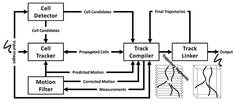
Our tracking system integrates five modules (Fig. 2), including: 1) cell detector, which detects and labels candidate cell regions in the input image utilizing region, edge, and shape information; 2) cell tracker, which propagates candidate cell regions and identities across frames using a fast topologically-constrained geometric active contour framework; 3) motion filter, which performs prediction and filtering of the cell motion dynamics using a biologically inspired adaptive interacting multiple models (IMM) filter; 4) track compiler, which generates intermediate result called track segments by fusing the output from the above modules, and judging on what is and what is not physically possible; and 5) track linker, which oversees the entire tracking history and establishes the complete cell trajectories and lineages. To achieve robust and versatile cell tracking, our system combines the advantages of both tracking-by-detection and tracking-by-model-evolution approaches (Section 2), while mitigating against their disadvantages. Before dwelling on each module, we provide an overview of the system workflow and establish notations.

Fig. 2.

System Overview

3.1 System Workflow

Our system starts with processing the input images sequentially. Its output is a complete spatiotemporal history of the cell trajectories, including cell centroid positions, cell migration velocities, shape and intensity parameters for every cell, as well as the parent-child relations between cells. For each cell, the system may generate multiple track segments as intermediate output. Each track segment is associated with a unique positive-integer label n. Each cell is identified using the label of its first track segment.

To initialize tracking, the cell detector detects all candidate cells in the first frame I₀(x, y) and generates an initial cell region labeling map ψ₀(x, y), where ψ₀(x, y) = n if pixel (x, y) is part of cell n, and ψ₀(x, y) = 0 if (x, y) belongs to the background. Subsequently, for each frame I_k(x, y), k = 1, 2…, K:

Step 1

The cell detector segments cell regions in the image using a combination of region-based and edge-based approaches. The output is a binary map of cell regions, denoted χ_k(x, y). Each connected foreground component in χ_k(x, y) is considered a cell candidate in frame k.

Step 2

The cell tracker propagates the cell region labeling ψ_k−1(x, y) from frame k − 1 to frame k. We extended a fast geometric active contour algorithm (Shi and Karl, 2005b) to segment cell regions and to propagate the corresponding cell labels. First, a level set function ϕ_k(x, y) is initialized using ψ_k−1(x, y). Then, ϕ and ψ are evolved together to minimize an “energy” functional that combines a region competition term (Zhu and Yuille, 1996), a geodesic edge term (Caselles et al., 1997), and a motion term based on the distribution of the predicted cell position from the motion filter. Topological constraints are incorporated to the level set evolution to prevent contours that represent different cells from merging. The output is the propagated cell labeling map for frame k, denoted ψ̂_k(x, y).

Step 3

The track compiler compares the outputs of the cell detector and the cell tracker, and takes one of the following actions: creates a new or daughter track segment, or updates an existing track, or terminates a track. For continuing track segments, the track compiler calls on the motion filter to update the cell motion state in frame k, and to predict its state for frame k + 1. The predictions will be useful for the track linking process (step 4), as well as for the level set evolution for the subsequent frame (step 5). For new track segments, initial motion states are initialized based on quantities measured from the corresponding cell regions. The output of this step includes the track segments and an updated region labeling map ψ_k(x, y).

Step 4

The track linker examines all track segments up to frame k, and detects whether two or more track segments correspond to one cell. It attempts to link track segments in the spatiotemporal image volume, and to form more complete cell trajectories. The updated cell trajectories are fed back to the track compiler for subsequent tracking in frame k + 1.

The following sections elaborate on each module of this system.

3.2 Cell Detection

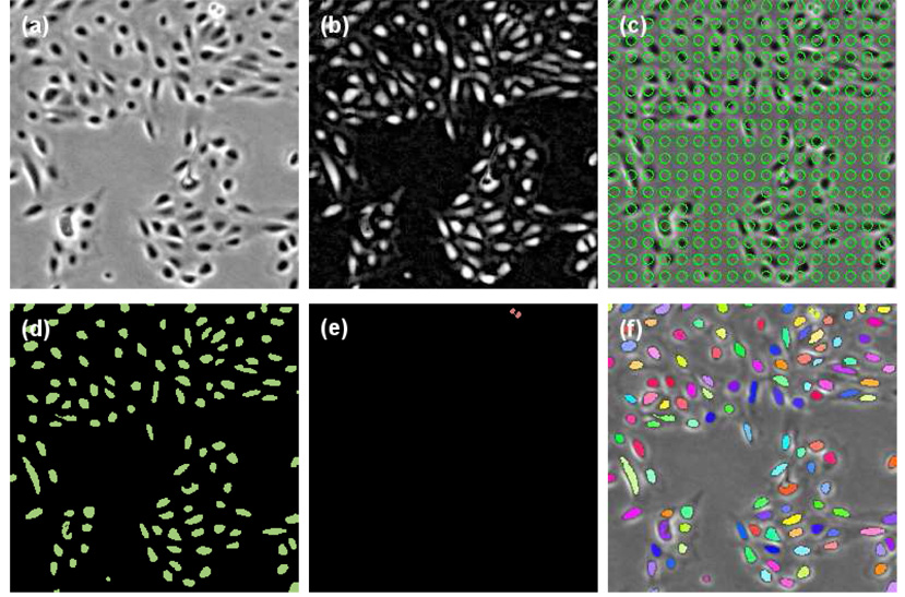
Cells in phase contrast microscopy normally appear as dark regions surrounded by bright halo artifacts, except for mitotic (dividing) or apoptotic (dying) cells, which appear rounder and brighter than the other cells. Consequently, the cell detector takes two approaches: 1) region-based detection, which employs a grayscale morphological filter and the level set method to extract non-mitotic and non-apoptotic cells; and 2) edge-based detection, which detects mitotic and apoptotic cells based on image edges, as well as a set of shape and appearance criteria. The outputs of the two approaches are combined to yield a binary image χ(x, y) : Ω → {0, 1}, in which each non-zero connected component is considered a cell candidate. The steps of cell detection are illustrated in Fig. 3, and detailed in the next two subsections.

Fig. 3.

Illustration of cell detection steps. Shown are the human amnion epithelial (AE) stem cells. (a) Original image I. (b) Result of rolling-ball filtering Î_r. (c) Green circles represent initial level set contour for region-based cell detection. (d) Region-based cell detection output χ_r. (e) Edge-based cell detection output χ_e. (f) Combined output with each cell region shown in a different color.

3.2.1 Region-Based Cell Detection

The region-based cell detection approach consists of two steps: 1) morphological pre-segmentation, the result of which is used to estimate the intensity distributions of cells and background; and 2) level set segmentation, which achieves more robust cell localization.

The rolling-ball filter (Sternberg, 1983) is applied to pre-segment the non-mitotic and non-apoptotic cells. The rolling-ball filter simulates rolling a ball beneath the intensity profile of an image, removing the peaks that are untouchable by the ball surface. It is a grayscale morphological filter that is related to the classical top-hat transformation (Meyer, 1979) by

$$I-\text{rollball}(I,r)=\text{tophat}(I,{\mathit{\text{ball}}}_r),$$

where r is the radius of the rolling ball, and ball_r is a non-flat half ball-shaped structuring element with radius r. The parameter r is set roughly equal to the average radius of cells to be detected. To apply the rolling-ball filter, the input image is first inverted such that the cell interior appears brighter than the surrounding halo. The operation Î_r = Ī − rollball(Ī, r) on the inverted image Ī will produce an image Î_r with cell regions solidified and highlighted. Otsu thresholding (Otsu, 1979) is then applied on Î_r to obtain a binary mask χ̂_r of the cell regions.

The binary mask χ̂_r constitutes a rough pre-segmentation of the image, which enables us to obtain two histograms: a cell histogram h_C, and a background histogram h_B. With these histograms, a Bayesian maximum a-posteriori probability (MAP) classifier can be implemented via the following test:

$$\text{Classify a pixel }I(x,y)\text{as}\{\begin{array}{cc}\text{cell},\hfill & \text{if}{h}_{\mathrm{C}}(I(x,y))>h_{\mathrm{B}}(I(x,y)),\hfill \\ \text{background},\hfill & \text{otherwise}.\hfill \end{array}$$ (1)

To understand this, recall that a MAP classifier can be expressed via the Bayes rule as: arg max_c p(c|I(x, y)) = arg max_c p(I(x, y)|c)p(c), where c ∈ {C,B} is the class label. The following relation holds:

$$\frac{p(I(x,y)|\mathrm{C})p(\mathrm{C})}{p(I(x,y)|\mathrm{B})p(\mathrm{B})}=\frac{h_{\mathrm{C}}(I(x,y))/m_{\mathrm{C}}·m_{\mathrm{C}}/m}{h_{\mathrm{B}}(I(x,y))/m_{\mathrm{B}}·m_{\mathrm{B}}/m}=\frac{h_{\mathrm{C}}(I(x,y))}{h_{\mathrm{B}}(I(x,y))},$$

where m_C = sum(h_C) is the number of pixels in the cell regions, m_B = sum(h_B) is the number of pixels in the background, and m = m_C + m_B is the total number of pixels in the image.

Instead of a direct application of Equation (1), the MAP classifier is implemented via the level set method (Osher and Sethian, 1988), which is less sensitive to noise and yields robust segmentation. The method will be elaborated in Section 3.3. After level set segmentation, an a priori size constraint is imposed by removing the connected components with sizes smaller than s_min pixels or larger than s_max pixels. The output is a binary map of segmented cell regions χ_r.

3.2.2 Edge-Based Cell Detection

The edge-based cell detection approach aims to detect mitotic and apoptotic cells, which appear rounder and brighter than the other cells. This approach consists of three steps. First, the Canny edge detector (Canny, 1986) is applied to compute an edge map of the image. Then, the regions that are enclosed by edges are located and filled. The regions whose sizes fall outside the valid range of [s_min, s_max] (Section 3.2.1) are discarded. Then, for each remaining region, the mean pixel intensity μ_o in a w-pixel-wide rim of the region and the eccentricity are computed. The eccentricity is measured by fitting an ellipse to the region using second-moment matching and computing the ratio of the distance between the foci of the ellipse and its major axis length. Finally, the regions with eccentricities smaller than 0.95 and μ_o > μ_N + σ_N are selected as cell regions, where μ_N and σ_N are respectively the mean and standard deviation of the pixel intensities in a neighborhood of radius r_N surrounding the region. The parameters w and r_N are set to w = max(1, r/3) and r_N = 4r in our implementation, where r is defined in Section 3.2.1. The output is a binary map χ_e of mitotic and apoptotic cells.

3.3 Geometric Active Contour Cell Tracker

Because cells are highly-deformable objects and may divide over time, we choose to represent cell boundaries using an implicit contour model, commonly known as the geometric active contour model. In this model, the boundary of each cell is considered as a closed contour C in the image domain Ω ∈ ℝ². Its contour is represented as the zero level line of a time-dependent embedding function ϕ : Ω × [0, T] → ℝ, where

$$C(t)=\{(x,y)\in \mathrm{\Omega }|\varphi (x,y,t)=0\},$$

such that ϕ(C(t), t) = 0 at any time. Evolving the embedding function ϕ over time is an elegant method to keep track of the motion of the boundary, including its topological changes such as splitting and merging.

Among various approaches to evolve a geometric active contour, the most popular one is the level set method (Osher and Sethian, 1988), in which one evolves the embedding function (or the level set function) ϕ according to an appropriate partial differential equation (PDE). The PDE is usually derived as the Euler-Lagrange equation:

$$\frac{\partial \varphi }{\partial t}=-\frac{\partial E(\varphi )}{\partial \varphi },$$ (2)

which minimizes an application-specific “energy” functional E(ϕ).

For cell tracking, the energy functional is constructed such that its minimization leads to the propagation of cell boundaries from frame k − 1 to frame k. The propagated cell boundaries should not only match the cell appearances in frame k, but also be consistent with the cell motion pattern. The energy consists of a weighted sum of three terms, which are derived from: 1) the image region statistics (E_region); 2) the image edges (E_edge); and 3) the prediction of cell motion (E_motion):

$$E=E_{\text{region}}+w_{\text{edge}}{E}_{\text{edge}}+w_{\text{motion}}{E}_{\text{motion}},$$ (3)

where w_edge ≥ 0 and w_motion ≥ 0 are weighting coefficients. The dependency on ϕ is omitted in the notation for simplicity. The energy terms implicitly depend on ϕ, which will be further explained in Section 3.3.3.

N_k−1 is the set of cells to be propagated from frame k − 1 to frame k. Each cell n ∈ N_k−1 occupies the region Ω_n ⊂ Ω, enclosed by its boundary C_n = {(x, y)|(x, y) ∈ ∂Ω_n}. The region that is not occupied by cells is the background, denoted by Ω₀.

The region energy E_region is based on the Bayesian region-competition framework (Zhu and Yuille, 1996; Cremers et al., 2007):

$$\begin{array}{cc}{E}_{\text{region}}=\hfill & -{\displaystyle \sum _{n\in {\mathbf{N}}_{k-1}}{\displaystyle \int {\displaystyle {\int }_{{\mathrm{\Omega }}_n}\text{log}}p({\mathrm{\Omega }}_n|I_k(x,y))dxdy}}\hfill \\ \hfill & -{\displaystyle \int {\displaystyle {\int }_{{\mathrm{\Omega }}_0}\text{log}}p({\mathrm{\Omega }}_0|I_k(x,y))dxdy}+\frac{\nu }{2}{\displaystyle \sum _{n\in {\mathbf{N}}_{k-1}}{\displaystyle {\int }_{C_n}dl.}}\hfill \end{array}$$ (4)

It represents the joint posterior probability that each pixel in frame k belongs to a certain propagated region (first two terms), subject to a penalty on the total length of the region boundaries (third term). The parameter ν specifies the strength of the penalty.

The edge energy E_edge measures the edgeness along the region boundaries. It is formulated following the approach of geodesic active contours (Caselles et al., 1997; Goldenberg et al., 2001), which can be interpreted as the length of a curve in a Riemannian space whose metric is induced by the image edges:

$$E_{\text{edge}}={\displaystyle \sum _{n\in {\mathbf{N}}_{k-1}}{\displaystyle {\int }_{C_n}e(C_n)dl.}}$$ (5)

The function e(·) is the edgeness metric, which is ideally zero at the locations of image edges, and takes on larger values elsewhere.

The motion energy E_motion represents the joint probability that the cell regions reside at the locations predicted by their respective motion filters:

$$E_{\text{motion}}=-{\displaystyle \sum _{n\in {\mathbf{N}}_{k-1}}{\displaystyle \int {\displaystyle {\int }_{{\mathrm{\Omega }}_n}\tau +\text{log}}}{\widehat{p}}_{k|k-1}(x,y|{\mathrm{\Omega }}_n)}dxdy.$$ (6)

Here, τ > 0 is a size-constraint parameter, which is necessary because log p̂_k|k−1 is non-positive everywhere, and because the contour that minimizes E_motion will enclose the entire image if τ = 0. In addition to providing motion context, the distribution p̂_k|k−1(x, y|Ω_n) serves as an implicit shape prior. The definition of p̂_k|k−1(x, y|Ω_n) will be further discussed in Section 3.3.3.

For tracking N > 1 cells in parallel, one key issue is how to uniquely identify each cell region using the implicit contour representation. A straightforward solution is to utilize N level set functions (Brox and Weickert, 2006; Mansouri et al., 2006), each of which represents one cell. This solution, however, is highly inefficient for simultaneously tracking thousands of cells. Inspired by the approaches in (Feng et al., 2001; Shi and Karl, 2005b), we chose to represent all regions using one level set function ϕ, and to keep track of the identities of cell regions by evolving the region labeling function ψ (Section 3.1) simultaneously with the level set function ϕ. The implementation of our approach will be detailed in the next three sections.

3.3.1 Euler-Lagrange Equations

The first step towards tracking is to rewrite the energy terms such that they explicitly depend on ϕ. We introduce three auxiliary functions: the region indicator function R_n(·), the Heaviside function H(·), and the one-dimensional Dirac measure δ(·), defined as follow:

$$R_n(\psi )=\{\begin{array}{c}1,\text{if}\psi =n,\hfill \\ 0,\text{if}\psi \ne n,\hfill \end{array}H(\varphi )=\{\begin{array}{c}1,\text{if}\varphi \ge 0,\hfill \\ 0,\text{if}\varphi <0,\hfill \end{array}\delta (\varphi )=\frac{d}{d\varphi }H(\varphi ),$$

where ϕ < 0 applies to points inside the cell regions, and ϕ > 0 for points in the background. The energy terms can now be rewritten as:

$$\begin{array}{cc}{E}_{\text{region}}=\hfill & -{\displaystyle \sum _{n\in {\mathbf{N}}_{k-1}}{\displaystyle \int {\displaystyle {\int }_{\mathrm{\Omega }}{R}_n(\psi )(1-H(\varphi ))\text{log}p({\mathrm{\Omega }}_n|I_k)dxdy}}}\hfill \\ \hfill & -{\displaystyle \int {\displaystyle {\int }_{\mathrm{\Omega }}H(\varphi )\text{log}p({\mathrm{\Omega }}_0|I_k)dxdy}+\frac{\nu }{2}{\displaystyle \sum _{n\in {\mathbf{N}}_{k-1}}{\displaystyle \int {\displaystyle {\int }_{\mathrm{\Omega }}\delta (\varphi )|\nabla \varphi |dxdy}}}}\hfill \end{array}$$ (7)

$$E_{\text{edge}}={\displaystyle \int {\displaystyle {\int }_{\mathrm{\Omega }}\delta (\varphi )|\nabla \varphi |edxdy}}$$ (8)

$$E_{\text{motion}}={\displaystyle \sum _{n\in {\mathbf{N}}_{k-1}}{\displaystyle \int {\displaystyle {\int }_{\mathrm{\Omega }}{R}_n(\psi )(1-H(\varphi ))(\tau +\text{log}{\widehat{p}}_{k|k-1}(x,y|{\mathrm{\Omega }}_n))dxdy.}}}$$ (9)

Herein, the dependency on (x, y) is omitted in the notations for simplicity.

Then, by computing the first variation ∂E(ϕ)/∂ϕ and by substituting it into Equation (2), the Euler-Lagrange equation for minimizing the energy can be obtained. The equation can be written in the following standard form:

$$\frac{\partial \varphi }{\partial t}=-F\delta (\varphi ),\text{where}F=F_{\text{region}}+w_{\text{edge}}{F}_{\text{edge}}+w_{\text{motion}}{F}_{\text{motion}}.$$ (10)

The speed functions F_region, F_edge, and F_motion are defined as:

$$F_{\text{region}}={\displaystyle \sum _{n\in {\mathbf{N}}_{k-1}}\text{log}}p({\mathrm{\Omega }}_n|I_k)R_n(\psi )-\text{log}p({\mathrm{\Omega }}_0|I_k)+\frac{\nu }{2}\kappa$$ (11)

$$F_{\text{edge}}=\nabla e·\nabla \varphi /|\nabla \varphi |+e\kappa$$ (12)

$$F_{\text{motion}}={\displaystyle \sum _{n\in {\mathbf{N}}_{k-1}}(\text{log}{\widehat{p}}_{k|k-1}(x,y|{\mathrm{\Omega }}_n)-\tau )R_n(\psi )}$$ (13)

where

$$\kappa =\nabla ·\frac{\nabla \varphi }{|\nabla \varphi |}$$ (14)

is the mean curvature.

3.3.2 Contour Merging Avoidance by Topology Constraints

The topological flexibility of the implicit contour representation not only facilitates the tracking of cell divisions, but also permits the merging of contacting objects. This may cause two adjacent objects in one frame to falsely merge into one object in the next frame. In the context of cell tracking, the merging of multiple cells would signify cell fusion. While cell fusion occurs in specific cell types (e.g. activated macrophages and osteoclasts), it does not normally occur for the cell types studied in this paper, nor in many other studies (Zimmer et al., 2002; Mukherjee et al., 2004; Zhang et al., 2004; Yang et al., 2005a; Zimmer and Olivo-Marin, 2005; Debeir et al., 2005; Al-Kofahi et al., 2006; Bunyak et al., 2006; Nath et al., 2006). To prevent false cell fusion, it is important to incorporate a topological constraint that permits division but prohibits merging.

To introduce the topological constraint, we borrow the concept of topological numbers from digital topology (Han et al., 2003). Let N₈(x, y) be the set of 8 neighbors of pixel (x, y). The topological number of (x, y) with respect to the cell region Ω_n (n > 0), denoted T_n(x, y), is the number of 4-connected components in the set Ω_n ∩ N₈(x, y). Similarly, the topological number of (x, y) with respect to the background Ω₀, denoted T₀(x, y), is the number of 8-connected components in the set Ω₀ ∩ N₈(x, y). Let o(x, y) denote the number of cell regions that overlap with N₈(x, y). Then, the relaxed topological number (Shi and Karl, 2005b) for pixel (x, y) is defined as:

$$T_{\mathrm{r}}(x,y)=\text{min}\left[o(x,y),\text{max}\left(T_n(x,y),T_0(x,y)\right)\right].$$

The boundaries of two different cell regions can merge only if the level set function changes sign from positive to negative at a point (x, y) with T_r(x, y) > 1. By detecting the points at which T_r > 1, and preventing the level set function from changing sign at these points during the contour evolution, merging of different cell regions can be effectively prevented.

3.3.3 Fast Implementation

Traditional implementations of the level set method require evaluating PDEs (e.g. Equation (10)) using numerical methods (e.g., finite difference), which is computationally expensive. Among various approaches to speed up the computation (Cates et al., 2004; Lefohn et al., 2004; Pan et al., 2006), the fast two-cycle algorithm proposed in (Shi and Karl, 2005a,b) is chosen, since it achieves near real-time tracking speed, allows straightforward incorporation of topological constraints, and is easy to implement.

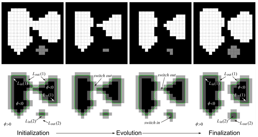
The algorithm evolves a contour iteratively by operations as simple as switching elements between two linked lists, L_in and L_out, which keep track of the points adjacent to the contour. This approach can be viewed as an extreme case of the narrow-band scheme with a two-pixel bandwidth (Chopp, 1993; Sethian, 1999). For tracking N contours, 2N linked lists are initialized from the region labeling map ψ(x, y) according to:

$$\begin{array}{cc}\hfill L_{\text{out}}(n)& =\{\mathbf{x}|\psi (\mathbf{x})=n,\exists {\mathbf{x}}^{*}\in N_4(\mathbf{x})\text{where}\psi ({\mathbf{x}}^{*})\ne n\},\hfill \\ \hfill L_{\text{in}}(n)& =\{\mathbf{x}|\psi (\mathbf{x})=n,\exists {\mathbf{x}}^{*}\in N_4(\mathbf{x})\text{where}{\mathbf{x}}^{*}\in L_{\text{out}}(n)\},\hfill \end{array}$$ (15)

where x ≡ (x, y). Accordingly, the level set function is defined as:

$$\varphi (x,y)=\{\begin{array}{cc}\hfill 3,& \text{if}(x,y)\text{is an exterior pixel},\hfill \\ \hfill 1,& \text{if}(x,y)\in L_{\text{out}}(n),\forall n,\hfill \\ \hfill -1,& \text{if}(x,y)\in L_{\text{in}}(n),\forall n,\hfill \\ \hfill -3,& \text{if}(x,y)\text{is an interior pixel},\hfill \end{array}$$ (16)

which approximates a signed distance function.

Each contour-evolution iteration is performed in two cycles: an update cycle and a regulation cycle.

Update Cycle

The update cycle evolves the contour according to the sign of a speed function F̂, which approximates F given in Equation (10) with all curvature-dependent terms removed (i.e., the terms $\frac{\nu }{2}\kappa$in (11) and eκ in (12) are no longer necessary) :

$$\widehat{F}(x,y)={\widehat{F}}_{\text{region}}(x,y)+w_{\text{edge}}{\widehat{F}}_{\text{edge}}(x,y)+w_{\text{motion}}{\widehat{F}}_{\text{motion}}(x,y),$$ (17)

where

$${\widehat{F}}_{\text{region}}(x,y)=\{\begin{array}{cc}\hfill 1,& \text{if}\chi (x,y)>0,\hfill \\ \hfill -1,& \text{otherwise},\hfill \end{array}$$ (18)

$$\begin{array}{cc}{\widehat{F}}_{\text{edge}}(x,y)=\hfill & -(e(x+1,y)-e(x-1,y))(\varphi (x+1,y)-\varphi (x-1,y))\hfill \\ \hfill & +(e(x,y+1)-e(x,y-1))(\varphi (x,y+1)-\varphi (x,y-1)),\hfill \end{array}$$ (19)

$${\widehat{F}}_{\text{motion}}(x,y)={\displaystyle \sum _{n\in {\mathbf{N}}_{k-1}}(\text{log}}𝒩(x,y|{\widehat{\mathbf{z}}}_{n,k|k-1},{\mathbf{S}}_{n,k-1})-\tau )R_n(\psi (x,y)).$$ (20)

The region speed F̂_region requires the cell candidate map χ(x, y) output from the cell detector. Recall from Section 3.2 that χ(x, y) is computed by combining two approaches: region-based detection and edge-based detection. In region-based detection, the level set algorithm is executed using a uniform lattice-of-circles initialization and the following speed function:

$${\widehat{F}}^{*}(x,y)=h_{\mathrm{C}}(I_k(x,y))-h_{\mathrm{B}}(I_k(x,y)),$$ (21)

which implements the MAP classifier given in Equation (1). The output segmentation χ_r(x, y) is combined with the output from edge-based detection χ_e(x, y) by a binary OR operation to obtain χ(x, y).

The edge speed F̂_edge is a central-difference approximation of the first term of Equation (12). Inspired by (Huang et al., 2004), we define the edgeness function e(x, y) to be the Euclidean distance transform of the edge map of I_k(x, y), which is produced by the Canny edge detector. This definition induces fewer local minima as opposed to the gradient-based definition in (Caselles et al., 1997). The edge map is also utilized for edge-based cell detection (Section 3.2.2), hence this computation can be reused.

The function 𝒩 (·|z, S) in Equation (20) denotes a bivariate normal distribution with mean z and covariance S. The vector ẑ_n,k|k−1 is the centroid position of cell n in frame k predicted by the motion filter, which will be explained further in Section 3.4. S_n,k−1 is the shape matrix, computed as:

$${\mathbf{S}}_{n,k-1}=\text{cov}\{(x,y)|{\psi }_{k-1}(x,y)=n\}.$$ (22)

It can be considered as an elliptical approximation of the cell shape in frame k − 1 by second-moment matching.

Regulation Cycle

The regulation cycle provides smoothness regulation to the contour using local Gaussian filtering. This regulation has a similar effect as the curvature-dependent terms in Equation (11) and Equation (12), but avoids the expensive computation of the curvature. This is because the curvature equals ∇²ϕ (i.e., the Laplacian of ϕ) when ϕ is a signed distance function (|∇ϕ| = 1); and based on the theory of heat diffusion (Perona and Malik, 1990), evolving a function according to its Laplacian is equivalent to Gaussian filtering.

More detail of the implementation is provided in Appendix A with pseudocode. This algorithm is limited to a pixel-level accuracy unless the input image is interpolated. A pixel-level accuracy is adequate for our study, since our primary goal is to construct the cell trajectories over time, rather than to delineate the cell boundaries at a sub-pixel precision.

3.4 Interacting Multiple Models Motion Filter

A motion filter is the fundamental building block of many tracking systems (Ristic et al., 2004). It provides recursive estimations of the target states (such as position, speed, and acceleration) based on noisy measurements. Essential to any motion filter is a motion model that describes the target dynamics, and a measurement model that relates states to measurements. Traditional motion filters, such as the Kalman filter (Kalman, 1960) and the standard particle filter (Gordon et al., 1993), are bound to use only one motion model, which is inadequate for tracking biological cells because cell dynamics vary frequently with time. The interacting multiple models (IMM) filter (Blom, 1984), instead, is capable of incorporating multiple motion models in parallel, and it has been shown to be well suited for biological object tracking (Genovesio et al., 2006).

Cell motions are assumed to consist of a finite number of modes. Each mode can be described by a linear model with additive Gaussian noise. The motion models and the measurement model are defined as:

$$\begin{array}{cc}\hfill \text{Motion models}:& {\mathbf{s}}_k={\mathbf{F}}^i{\mathbf{s}}_{k-1}+{\mathbf{v}}_{k-1}^i,i\in \{,\dots ,M\}\hfill \\ \hfill \text{Measurement model}:& {\mathbf{z}}_k=\mathbf{H}{\mathbf{s}}_k+{\mathbf{w}}_k.\hfill \end{array}$$

Here, s_k is the state vector of a cell in frame k, which consists of the centroid position, velocity, and acceleration of the cell, i.e., s_k ≡ (x_k, ẋ_k, ẍ_k, y_k, ẏ_k, ÿ_k)^′. Note that the “prime” sign (’) denotes vector or matrix transposition. The corresponding measurement vector z_k ≡ (x_k, y_k)^′ contains the measured centroid position. Fⁱ is the state transition matrix of model i, and H is the measurement matrix that relates states to measurements. ${\mathbf{v}}_{k-1}^i\text{and}{\mathbf{w}}_k^i$ are the process and measurement noise vectors, which are uncorrelated zero-mean Gaussian processes with covariances Qⁱ and R, respectively.

The IMM filter operates M Kalman filters in parallel, each of which is matched to a distinct motion model. It assumes that the transition between models is regulated by a finite-state Markov chain, with probability p_ij of switching from model i to model j in successive frames. However, rather than making hard commitments to any single model, it maintains a weighting among the models, which is determined as the probability of each model being correct given the current measurement. Hence, the optimal state estimate at any time instant is a mixture of Gaussian distributions. Each mixture component is the estimate from a Kalman filter, weighted by the posterior probability of the corresponding motion model. This leads to a mixture with exponentially growing number of components in time because of the branching of model switching hypotheses. To avoid the combinatorial explosion and make the computation tractable, the IMM filter approximates the mixture of Gaussians with a single Gaussian with equal mean and covariances.

The filtering recursion consists of two stages: prediction and correction. The prediction stage predicts the state ŝ_k|k−1 at time k based on the state history up to time k − 1; the correction stage generates a refined estimate ŝ_k by incorporating the newly-arrived measurement z_k. The mechanisms of the two stages are detailed below.

Prediction

Starting from M weights ${\rho }_{k-1}^i$, states ${\widehat{\mathbf{s}}}_{k-1}^i$ and covariances ${\mathrm{\Sigma }}_{k-1}^i$ from the previous iteration, the mixed initial condition is computed:

$${\widehat{\mathbf{s}}}_{k-1}^{0j}={\displaystyle \sum _i{\rho }_{k-1}^{i|j}{\widehat{\mathbf{s}}}_{k-1}^i},$$ (23)

$${\mathrm{\Sigma }}_{k-1}^{0j}={\displaystyle \sum _i{\rho }_{k-1}^{i|j}\left[{\mathrm{\Sigma }}_{k-1}^i+\left({\widehat{\mathbf{s}}}_{k-1}^i-{\widehat{\mathbf{s}}}_{k-1}^{0j}\right){\left({\widehat{\mathbf{s}}}_{k-1}^i-{\widehat{\mathbf{s}}}_{k-1}^{0j}\right)}^{\prime }\right]},$$ (24)

where ${\rho }_{k-1}^{i|j}=p_{ij}{\rho }_{k-1}^i/{\rho }_{k|k-1}^j,\text{and}{\rho }_{k|k-1}^j={\sum }_i{p}_{ij}{\rho }_{k-1}^i$. These are input to M Kalman filters to compute the state prediction ${\widehat{\mathbf{s}}}_{k|k-1}^j$ and covariance ${\mathrm{\Sigma }}_{k|k-1}^j$:

$${\widehat{\mathbf{s}}}_{k|k-1}^j={\mathbf{F}}^j{\widehat{\mathbf{s}}}_{k-1}^{0j},$$ (25)

$${\mathrm{\Sigma }}_{k|k-1}^j={\mathbf{F}}^j{\mathrm{\Sigma }}_{k-1}^{0j}({\mathbf{F}}^j{)}^{\prime }+{\mathbf{Q}}^j.$$ (26)

The combined state and covariance predictions can be determined by:

$${\widehat{\mathbf{s}}}_{k|k-1}={\displaystyle \sum _j{\rho }_{k|k-1}^j}{\widehat{\mathbf{s}}}_{k|k-1}^j,$$ (27)

$${\mathrm{\Sigma }}_{k|k-1}={\displaystyle \sum _j{\rho }_{k|k-1}^j\left[{\mathrm{\Sigma }}_{k|k-1}^j+({\widehat{\mathbf{s}}}_{k|k-1}^j-{\widehat{\mathbf{s}}}_{k|k-1})({\widehat{\mathbf{s}}}_{k|k-1}^j-{\widehat{\mathbf{s}}}_{k|k-1}{)}^{\prime }\right]}.$$ (28)

The predicted centroid positions ẑ_k|k−1 = Hŝ_k|k−1 of all cells are fed to the cell tracker to guide the level set evolution in frame k (see Section 3.3.3).

Correction

Given the predicted states, covariances, and measurement z_k, the Kalman filters are used to obtain the updated state ${\widehat{\mathbf{s}}}_k^j$ and covariance ${\mathrm{\Sigma }}_k^j$.

$${\widehat{\mathbf{s}}}_k^j={\widehat{\mathbf{s}}}_{k|k-1}^j+{\mathbf{K}}_k^j({\mathbf{z}}_k-\mathbf{H}{\widehat{\mathbf{s}}}_{k|k-1}^j),$$ (29)

$${\mathrm{\Sigma }}_k^j={\widehat{\mathrm{\Sigma }}}_{k|k-1}^j-{\mathbf{K}}_k^j\mathbf{H}{\widehat{\mathrm{\Sigma }}}_{k|k-1}^j,$$ (30)

where ${\mathbf{K}}_k^j={\mathrm{\Sigma }}_{k|k-1}^j\mathbf{H\prime }{(\mathbf{H}{\mathrm{\Sigma }}_{k|k-1}^j\mathbf{H\prime }+\mathbf{R})}^{-1}$ is the Kalman gain. The likelihood that model j is activated in frame k is

$${\lambda }_k^j=\text{exp}\left[-\frac{1}{2}({\mathbf{y}}_k^j{)}^{\prime }{({\mathbf{S}}_k^j)}^{-1}{\mathbf{y}}_k^j\right]/\sqrt{2\pi \text{det}({\mathbf{S}}_k^j)},$$ (31)

where ${\mathbf{y}}_k^j=({\mathbf{z}}_k-{\widehat{\mathbf{z}}}_{k|k-1})$ is the innovation of Kalman filter j, and ${\mathbf{S}}_k^j$ is the associated covariance. Then, the combined state ŝ_k and covariance Σ_k estimates can be computed by Equation (27) and Equation (28), with ${\rho }_{k|k-1}^j$ replaced by ${\rho }_k^j={\rho }_{k|k-1}^j{\lambda }_k^j/({\displaystyle {\sum }_i{\rho }_{k|k-1}^i}{\lambda }_k^i)$.

To initialize the IMM filter, the system tracks each cell without motion filtering in the first three frames in which it appears. The measured cell centroid positions in these frames are used to initialize the cell state ŝ₀. The initial model weights ${\rho }_0^i$ are set to equal 1/M (i ∈ {1, …,M}), indicating the initial complete uncertainty as to which model is more correct. The definitions of the remaining filter parameters will be discussed in sections 3.4.1 and 3.4.2.

3.4.1 Motion Models

To adapt the IMM filter for cell tracking, cell motion models need to be defined by specifying the system matrices Fⁱ and H. Inspired by (Genovesio et al., 2006), we define four motion models (M = 4): random walk (RW), constant velocity (CV), constant acceleration (CA), and constant-speed circular turn (CT). They represent four typical modes of cellular motion: Brownian motion, constant-velocity migration, constant-acceleration migration, and turning. Compared to the approach of Genovesio et al, the circular turn model is a novel addition, since the amnion epithelial stem cells that we experimented with perform an interesting turning motion. Moreover, instead of interpreting the motion models as the extrapolation of cell positions (Genovesio et al., 2006), we explicitly incorporate velocity and acceleration components into the state vector, and derive the models based on state-space differential equations. The state-transition matrices corresponding to the RW, CV, CA and CT models are, respectively:

$${\mathbf{F}}^1=\left[\begin{array}{cccccc}1& 0& 0& 0& 0& 0\\ 0& 0& 0& 0& 0& 0\\ 0& 0& 0& 0& 0& 0\\ 0& 0& 0& 1& 0& 0\\ 0& 0& 0& 0& 0& 0\\ 0& 0& 0& 0& 0& 0\end{array}\right],{\mathbf{F}}^2=\left[\begin{array}{cccccc}1& T_s& 0& 0& 0& 0\\ 0& 1& 0& 0& 0& 0\\ 0& 0& 0& 0& 0& 0\\ 0& 0& 0& 1& T_s& 0\\ 0& 0& 0& 0& 1& 0\\ 0& 0& 0& 0& 0& 0\end{array}\right],{\mathbf{F}}^3=\left[\begin{array}{cccccc}1& T_s& \frac{T_s^2}{2}& 0& 0& 0\\ 0& 1& T_s& 0& 0& 0\\ 0& 0& 1& 0& 0& 0\\ 0& 0& 0& 1& T_s& \frac{T_s^2}{2}\\ 0& 0& 0& 0& 1& T_s\\ 0& 0& 0& 0& 0& 1\end{array}\right],$$

$${\mathbf{F}}_k^4=\left[\begin{array}{cccccc}1& \frac{\text{sin}({\theta }_k{T}_s)}{{\theta }_k}& \frac{1-\text{cos}({\theta }_k{T}_s)}{{\theta }_k^2}& 0& 0& 0\\ 0& \text{cos}({\theta }_k{T}_s)& \frac{\text{sin}({\theta }_k{T}_s)}{{\theta }_k}& 0& 0& 0\\ 0& -{\theta }_k\text{sin}({\theta }_k{T}_s)& \text{cos}({\theta }_k{T}_s)& 0& 0& 0\\ 0& 0& 0& 1& \frac{\text{sin}({\theta }_k{T}_s)}{{\theta }_k}& \frac{1-\text{cos}({\theta }_k{T}_s)}{{\theta }_k^2}\\ 0& 0& 0& 0& \text{cos}({\theta }_k{T}_s)& \frac{\text{sin}({\theta }_k{T}_s)}{{\theta }_k}\\ 0& 0& 0& 0& -{\theta }_k\text{sin}({\theta }_k{T}_s)& \text{cos}({\theta }_k{T}_s)\end{array}\right],$$

where T_s is the time between the measurements (i.e., the frame interval). The subscript k in the coordinated turn transition matrix ${\mathbf{F}}_k^4$ indicates that it is time varying. It depends on the angular turning rate θ_k, which can be computed from the velocity and acceleration vectors as ${\theta }_k=\sqrt{{\mathit{ẍ}}_k^2+{\mathit{ÿ}}_k^2}/\sqrt{{\mathit{ẋ}}_k^2+{\mathit{ẏ}}_k^2}$. We refer the reader to (Zarchan and Musoff, 2005; Herman, 2002) for detailed derivations of the state-transition matrices. The proposed motion models share a common measurement matrix:

$$\mathbf{H}=\left[\begin{array}{cccccc}1& 0& 0& 0& 0& 0\\ 0& 0& 0& 1& 0& 0\end{array}\right].$$

3.4.2 Parameter Estimation and Adaptation for IMM

With the system matrices defined, the noise covariances Qⁱ, R, and the initial error covariance matrix${\mathrm{\Sigma }}_0^i$ can be estimated from training sequences using the expectation-maximization (EM) algorithm (Bishop, 2007). The details of the EM-IMM parameter estimation procedure are presented in Appendix B. While EM also permits the estimation of Fⁱ and H, the resulting matrices may be in arbitrary forms and are difficult to interpret. With the predefined system matrices, we gain additional insight into the typical motion patterns of each cell. Namely, we can identify if the cell motion is predominated by Brownian motion, constant-velocity migration, accelerating migration, or turning motion based on the corresponding model weights ${\rho }_k^i$ computed by the IMM filter.

One important parameter yet to be specified is the Markovian model transition probabilities p_ij. By convention, p_ij can be arranged in an M × M transition probability matrix (TPM) P, with p_i denoting the i-th row of P. Traditionally, the TPM is almost always treated as a fixed design parameter chosen empirically. For many biological applications, however, a priori information about the TPM may be inadequate or lacking. Cellular motion could vary considerably or become unpredictable due to changes of experimental procedures, extracellular environments, cell densities, and/or cell types. Moreover, imposing an empirical TPM would contradict the very goal of biological discovery, i.e., to discover unknown cell behavioral variations.

With the above considerations, we chose to perform online minimum meansquare error estimation of the TPM. Various algorithms exist for our purpose, and we adopt the quasi-Bayesian algorithm (Jilkov and Li, 2004), which is simple to implement, numerically stable, and requires negligible computational overhead. The quasi-Bayesian estimation assumes that each row p_i of the TPM follows a Dirichlet prior distribution. The Dirichlet distribution is defined by:

$$p({\mathbf{p}}_i|a_{i1},\dots ,a_{iM})=\frac{\mathrm{\Gamma }(a_{i1}+\cdots +a_{iM})}{\mathrm{\Gamma }(a_{i1})\cdots \mathrm{\Gamma }(a_{iM)}}{\displaystyle \prod _{j=1}^M{p}_{ij}^{a_{ij}-1},}$$ (32)

with hyperparameters a_ij ≥ 0. The Dirichlet distribution naturally satisfies the unit simplex requirement ${\displaystyle {\sum }_{j=1}^M{p}_{ij}=1}$ and p_ij ∈ [0, 1], for all i. The parameters a_ij represent the unnormalized a priori TPM. If they are chosen as a_i1 = ⋯ = a_iM = 1 for any i, the corresponding Dirichlet distribution of p_i coincides with the uniform distribution. Therefore, if a priori knowledge about the TPM is unavailable, the quasi-Bayesian estimator can naturally be initialized with the noninformative (uniform) prior p_ij = 1/M using parameters a_ij = 1 (i, j = 1,…,M).

Algorithm 1.

Quasi-Bayesian TPM Estimation

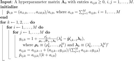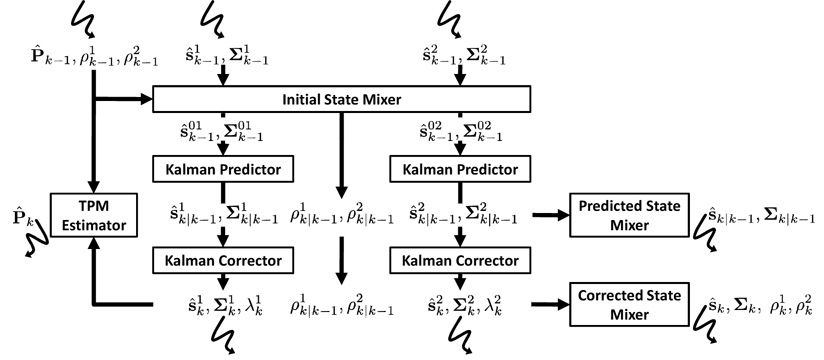
The quasi-Bayesian algorithm proceeds as follows. Upon receiving the first measurement z₁, a posterior probability p(p_i|z₁) can be obtained based on the Dirichlet prior p(p_i) for each model i, which is a weighted sum of M Dirichlet distributions. The posteriors over the subsequent measurements will be mixtures of exponentially more Dirichlet distributions. The quasi-Bayesian approach utilizes a similar approximation as in IMM to obtain a quasi-posterior distribution. At each time step, it approximates the posterior mixture of M Dirichlet distributions by a single Dirichlet distribution, then computes the quasi-posterior estimation p̂_i as the mean of this approximated distribution. This process is elaborated in (Jilkov and Li, 2004; Smith and Makov, 1978), and can be summarized as a recursive algorithm (Algorithm 1). The quasi-Bayesian algorithm integrates seamlessly with IMM, enabling us to update the TPM after the correction step in each filtering cycle (see Section 3.4). A diagram of the TPM-adaptive IMM filter with two models is given in Fig. 4.

Fig. 4.

Block diagram of the TPM-adaptive IMM filter framework for two models.

3.5 Track Compilation

The track compiler coordinates the cell detector, cell tracker and motion filter to produce track segments. We use N_k to denote the set of labels of all track segments created up to frame k. A track segment is active in frame k if it was successfully tracked in frame k − 1, otherwise it becomes inactive. Let Ω₀ denote the background region, and Ω_n denote the cell region with label n. An outline of the track compilation algorithm is shown in Algorithm 2.

Algorithm 2.

Track Compilation

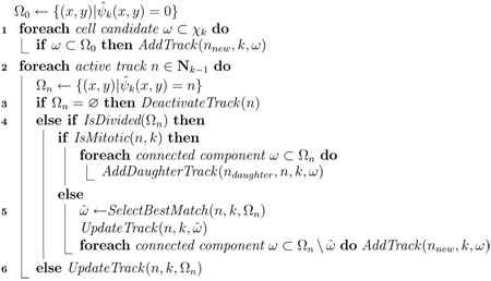The compiler first compares the output of the cell detector and cell tracker, χ_k(x, y) and ψ̂_k(x, y). Each cell candidate in χ_k(x, y) that does not overlap with any propagated cell region in ψ̂_k(x, y) is considered a new cell. A new track segment will be initialized, and ψ̂_k(x, y) will be updated accordingly.

Next, the algorithm scans through all active track segments, and deactivates track segments whose labels are not found in the propagated region labeling ψ̂_k(x, y). A track segment whose corresponding propagated cell region contains only one connected component will be updated directly. If a cell region consists of more than one connected components separated by a minimum distance d_min, the track compiler will judge between two possibilities: 1) the cell divided into daughter cells; or 2) one or more of these components are from occluded cells or close-by newly-entered cells. The algorithm will either create daughter tracks or continue tracking using the component that best matches the cell trajectory, depending on whether the cell is previously detected to be mitotic.

Details of several key operations are as follow.

AddTrack(ω, n_new, k) creates a new track segment labeled n_new; fills region ω with n_new; and initializes the cell state based on measurements of ω.

UpdateTrack(n, k, ω) updates the track segment n using the features of region ω, including the centroid location, mean intensity, area, and eccentricity. The centroid and the mean intensity are fed to the motion filter to obtain a filtered state of cell n in frame k. The last three features are used to classify a cell as normal, mitotic, or apoptotic, using three-nearest-neighbor (3NN) matching with the Mahalanobis distance to a set of training samples obtained off-line.

AddDaughterTrack(n_daughter, n, k, ω) creates a daughter track of cell n with a unique label n_daughter, and fills the region ω with n_daughter. The state of the daughter cell will be computed based on the measured centroid location and mean intensity of ω, and the predicted state of cell n.

SelectBestMatch(n, k, Ω_n) selects component ω̂ ∈ Ω_n that best matches the dynamics of cell n, i.e., the one which maximizes the innovation likelihood given by Equation (31) among all dynamic models.

IsDivided(Ω_n) returns true if region Ω_n has multiple connected components and the minimum distance between any two points in different components is greater than a preset threshold d_min; otherwise, it returns false.

IsMitotic(n, k) returns true if cell n is classified as mitotic during the past T frames using the approach described in UpdateTrack above.

The parameters d_min and T involved in the algorithm need to be adjusted for specific datasets. Their values will be provided in Section 4.2.

3.6 Track Linking

The track linker module provides the global view. It oversees the entire tracking history, and it detects potential problems among all track segments up to frame k based on two physical constraints: 1) a cell does not vanish unless it leaves the field-of-view, dies and is released into the media, or is occluded; and 2) a cell does not appear unless it enters from outside, divides from another cell, or comes out of occlusion. The linker attempts to correct violations of these constraints by linking track segments into complete cell trajectories, utilizing spatiotemporal context.

The track linking procedure is outlined in Algorithm 3. Here, N_lost ≡ {n_l|l = 1,…,L} denotes the label set of track segments that end before frame k, and N_found ≡ {n_f|f = 1,…,F} denotes the label set of track segments that start after the first frame. Most operations in the algorithm are self-explanatory. One vital step is the matching between lost and appearing track segments: MatchTracks (Line 4).

Algorithm 3.

Track Linking

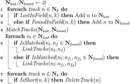In MatchTracks, a bipartite graph G is created, whose nodes correspond to the labels in N_lost and N_found. For each node pair (n_l, n_f), an arc 〈n_l, n_f〉 is created between node n_l and node n_f if the last centroid location (x_l, y_l, k_l) of track n_l is within a spatiotemporal double cone centered at the first centroid location (x_f, y_f, k_f) of track n_f , i.e.,

$$\begin{array}{c}\sqrt{{(x_l-x_f)}^2+{(y_l-y_f)}^2}\le |k_l-k_f|R+R_0,\text{and}\\ |k_l-k_f|\le D/2,\end{array}$$

where D, R and R₀ are user-defined parameters. Each arc 〈n_l, n_f〉 is assigned a weight $w_{lf}={\lambda }_{n_l{k}_f}^{\text{max}}(n_{f)}$, which is the maximum innovation likelihood of track n_l on the measurement of track n_f in frame k_f (Equation (31)). Intuitively, w_lf indicates how likely track segment n_f is a continuation of track segment n_l based on the dynamics of track n_l.

Next, a maximum-likelihood matching is computed between tracks n_l and n_f. The approach we reported previously (Li et al., 2007) only considered one-to-one matches. Hence, it could not handle the case where a cell is lost during mitosis, and whose daughter cells are re-detected in later frames. To handle this case, we improved the algorithm to consider both one-to-one and one-to-two matches. The algorithm relies on two inputs: an H × (L + F) constraint matrix C and an H × 1 likelihood vector d. Here, H is the total number of one-to-one and one-to-two matching hypotheses. L and F are, respectively, the numbers of track segments in N_lost and N_found. Matrix C and vector d are constructed as follows:

For each arc 〈n_l, n_f〉 in G, a new row is appended to C and a corresponding new element to d. Let h be the index of this new row. We set d(h) = w_lf, and

$$\mathbf{C}(h,i)=\{\begin{array}{cc}1,\hfill & \text{if}i=l\text{or}i=L+f,\hfill \\ 0,\hfill & \text{otherwise}.\hfill \end{array}$$

For each node n_l that is connected to multiple nodes n_f1,…,n_fm ∈ N_found (m ≥ 2), all possible one-to-two matchings are enumerated, e.g., n_l → (n_f1, n_f2), n_l → (n_f1, n_f3), and so on. For each of these hypotheses, say n_l → (n_f1, n_f2), a new row with index h′ to C and a corresponding new element is appended to d. The value of d(h′) is set to be the maximum innovation likelihood of track n_l for the spatiotemporal mean of the starting points of tracks n_f1 and n_f2, with the constraint

$$\mathbf{C}(\mathrm{h\prime },i)=\{\begin{array}{cc}1,\hfill & \text{if}i=l,i=L+f_1,\text{or}i=L+f_2,\hfill \\ 0,\hfill & \text{otherwise}.\hfill \end{array}$$

With C and d constructed, the matching problem reduces to selecting a subset of rows of C such that the sum of corresponding elements in d is maximized, under the constraint that no two rows share common nonzero entries. This can be posed as the following integer programming problem:

$$\underset{\mathbf{x}}{\text{max}}\mathbf{d\prime }\mathbf{x},\text{such that}\mathbf{C\prime }\mathbf{x}\le \mathbf{1},$$ (33)

where 1 is a H × 1 vector of ones. x is a H × 1 binary vector to be solved for, with x(h) = 1 if row h is selected in the solution, or x(h) = 0 otherwise. While integer programming problems are in general NP-hard, the problem given in Equation (33) can be solved exactly using linear programming. This is due to the fact that the constraint matrix C is totally unimodular², and the right-hand sides of the constraints are all integers. In fact, if the above two conditions are satisfied, a linear programming problem will always have an integer-valued solution (Papadimitriou and Steiglitz, 1998). In our implementation, the open-source software package lpsolve (Berkelaar et al., 2007) is used to solve the above integer programming problem. A similar optimization approach was used by Al-Kofahi et al (Al-Kofahi et al., 2006) for inter-frame cell matching. As an optional step after the completion of the track linking procedure, all cell trajectories that terminate in the field-of-view with lengthes shorter than a preset threshold will be regarded as noise and removed (Line 7).

4 Experimental Methods

The tracking system is implemented in ISO C++. The inputs to the system are gray-scale image sequences generated by the imaging software QED Image (Media Cybernetics Inc.). Unprocessed microscopy images are often distorted by spatial illumination inhomogeneity. The distortion is especially severe when low-magnification objectives are used. To normalize illumination, a flat-field correction filter is applied to the input images. This filter divides each input frame by a preacquired light field image, and then it scales the output pixel values to a fixed range. In our experiments, a light field image is unavailable. Therefore, a pseudo light field is generated for each sequence by applying a Gaussian filter with standard deviation of 50 to the first frame.

4.1 Data

The performance of our system is quantitatively evaluated on eight phase-contrast microscopy image sequences. They are categorized into three data sets (A, B and C) according to the cell type, imaging protocol and cell seeding method.

Dataset A includes two image sequences of MG-63 human osteosarcoma cells acquired with a 12-bit Qimaging Retiga EXi Fast 1394 CCD camera mounted on a Zeiss Axiovert 135 TV microscope, at a time-lapse interval of 4 minutes for 10 hours. Each sequence consists of 150 frames, with a frame dimension of 1280×1024 pixels, and a resolution of 1.9 µm/pixel at 4.9× magnification. The cells are seeded randomly on a polystyrene dish. The images are cropped to a size of 512×512 pixels (Fig. 1(a)) to speed up processing and evaluation. The cell populations in the cropped sequences are in the range of 80–110 cells per frame. An independent sequence of the same cell type was utilized for training.

Dataset B includes four image sequences of proprietary amnion epithelial (AE) stem cells (Fig. 1(b)), acquired using the same imaging protocol as Dataset A, except that the acquisition rate is one frame per 10 minutes. The AE cells are extracted from the placenta following live birth, and are potentially a noncontroversial source of stem cells for cell transplantation and regenerative medicine (Miki et al., 2005). The sequences were acquired over a duration of 42.5 hours, each consisting of 256 frames with 1280×1024 pixels/frame. The cell population density in each sequence is roughly 2000–5000 cells per frame, and is nearly confluent towards the end of the sequence. An independent sequence of the same cell type was utilized for training.

Dataset C includes one sequence of MG-63 cells (Fig. 1(c)) recorded by an 8-bit CCD camera on a Zeiss IM35 microscope. The sequence lasts for 43.5 hours and has a frame interval of 15 minutes, corresponding to 174 frames/sequence. The frame dimension is 512×512 pixels with a resolution of 3.9 µm/pixel at 5:1 magnification. The cells are seeded randomly on a fibrin-coated slide, on which a 0.75×0.75 mm² uniformly-concentrated square pattern of FGF-2 was created using our bioprinter (Weiss et al., 2005). The cell population in the sequence is in the range of 350–750 cells per frame. The first 40 frames of the sequence are reserved for training, the rest is used for testing.

In addition to the above datasets, 35 sequences of AE cells were utilized to qualitatively assess the tracking performance of the system.

4.2 Parameters

Many parameters involved in our system can be learned automatically from training data. These trainable parameters include the process noise covariances Qⁱ (i = 1,…,4), measurement noise covariance R, initial estimation error covariance ${\mathrm{\Sigma }}_0^i$ (i = 1,…,4), and the model transition probability matrix (TPM) P, all of which are required by the IMM motion filter. For each dataset, the parameters are learned using a set of manually tracked cell trajectories. The training set include 71 trajectories from dataset A, 101 trajectories from dataset B, and 232 trajectories from dataset C.

The training procedure alternates between two steps. First, Qⁱ, R, and ${\mathrm{\Sigma }}_0^i$ are trained using the EM-IMM algorithm (Appendix B) with an initial TPM P₀. This TPM has diagonal entries p_ii,0 = 0.85 and off-diagonal entries p_ij,0 = 0.05, (i ≠ j), which encodes the assumption that a cell tends to stay in a motion mode rather than to switch to the other modes in successive time steps. It is chosen instead of a uniform (uninformative) initialization as suggested in Section 3.4.2 because it leads to better capability of model identification and faster convergence of the parameters. Then, once Qⁱ, R, and ${\mathrm{\Sigma }}_0^i$ are learned, the TPM is re-estimated using the Quasi-Bayesian algorithm (Algorithm 1) with the hyperparameter matrix A₀ set to equal the previous P. The procedure iterates until the TPM converges.

The above procedure converges to a near identical TPM for all datasets, which approximately equals:

$$\mathbf{P}=\left[\begin{array}{cccc}0.9793& 0.0074& 0.0064& 0.0070\\ 0.0072& 0.9834& 0.0037& 0.0056\\ 0.0272& 0.0281& 0.9156& 0.0290\\ 0.0276& 0.0296& 0.0279& 0.9148\end{array}\right]$$ (34)

In addition to the tendency for cells to stay unchanged in a motion mode, the TPM indicates that the random walk and constant-velocity motions are more persistent, whereas the acceleration and turning motions are relatively transient. It is used to initialize the hyperparameter matrix A₀ in the subsequent experiments. In contrast to the TPM, the learned values of Qⁱ, R, and ${\mathrm{\Sigma }}_0^i$ vary between different datasets. Their specific values are less informative than the TPM, and are omitted here.

The settings of the additional parameters are summarized in Table 1. These parameters can be intuitively determined based on direct observation. For example, the cell detector parameter r is set to roughly equal to the average cell radius. The size constraints s_min and s_max loosely correspond to the expected cell size range. The cell tracker parameters w_edge, w_motion, and τ are determined empirically, and they are mostly held constant for different datasets. The parameter T is related to the maximum duration of mitosis events. The track linker parameters D, R, and R₀ are constrained by the maximum cell migration speed.

Table 1.

Summary of parameter settings for each dataset.

Dataset	r	smin	smax	wedge	wmotion	τ	dmin	T	D	R	R0
A	10	16	4000	0.1	0.1	0.001	10	10	10	5	10
B	5	5	2500	0.1	0.2	0.001	8	10	10	5	20
C	4	4	1000	0.1	0.1	0.001	3	5	6	3	5

4.3 Cell Detection Accuracy Assessment

To quantitatively evaluate cell detection accuracy, the centroid positions of all visible cells in 5 randomly selected images in each dataset were manually identified using an interactive program. The human operators can navigate through contextual frames to better identify overlapping cells, and to distinguish cells from background and other objects (e.g., glass scraps, air bubbles, etc.) that may exist in the field.

The detection accuracy is gauged using two metrics: 1) precision, which is the ratio of the number of detected cells to the total number of detected objects, and 2) recall (a.k.a. sensitivity), which is the ratio of the number of detected cells to the total number of cells actually in the image, visually determined by the human observer. In terms of true positives (TPs), false positives (FPs), true negatives (TNs) and false negatives (FNs), the metrics can be computed as: precision = TP/(TP + FP) and recall = TP/(TP + FN).

4.4 Cell Tracking Accuracy Assessment

The image sequences used for cell tracking accuracy assessment were selected to be feasible for manual tracking. Only the cells that appear in the initial frame of each sequence and their progeny were manually tracked. The manual tracking results were obtained after weeks of expert scrutiny, and gained consensus among multiple observers. The manually and automatically tracked trajectories (branches) were paired in the initial frame of each sequence, and they were compared in the remaining frames. An automatically tracked cell trajectory is considered valid only if it follows the same cell through all the frames that the cell appears. Any swapping of identities between two nearby cells will invalidate the trajectories of both cells and their progeny.

The sequences in datasets B and C contain hundreds to thousands of cells per frame, making it unrealistic to manually track all cells in the entire sequences. To make quantitative validations feasible, a 256×256-pixel region of interest (ROI) is defined in each image sequence of dataset B, and a 192×192-pixel ROI in dataset C. The automated tracking results are manually examined only within the ROI volume. In addition to the tracking validity defined previously, the ratio of cell divisions that were correctly tracked by the tracking system was also evaluated. This ratio is referred to as the division tracking ratio. A division is considered to be correctly tracked if the daughter cells are correctly located and the cell lineage is successfully established.

5 Results

5.1 Tracking Examples

Before presenting quantitative results, we provide several explanative examples to demonstrate the key features of our system.

Fig. 5 demonstrates that the topology-constrained level set can effectively prevent merging of closely contacting cells and maintain cell identities. In addition, cells (e.g., cell 25) are automatically initialized when they enter, and they (e.g. cells 16 and 20) are removed when they exit the field of view. This example is cropped from one of the sequences in dataset B.

Fig. 5.

Tracking contacting and partially overlapping AE cells. The numbers at the top-left corner are the frame indices. Cells 12, 15 and 18 are partially overlapping in frames 151–152. Cells 15 and 12 are closely passing each other in frames 162–167.

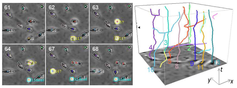
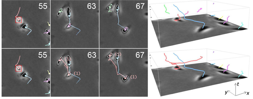
Fig. 6 shows an example of tracking mitotic and apoptotic cells. The images are taken from dataset C. Since the appearances of mitotic and apoptotic cells are almost identical during a certain period (frames 62 and 63), they can only be distinguished with sufficient temporal information (frames 64–68). This example illustrates that our tracking system can effectively detect mitoses and apoptoses, and distinguish between them by using the temporal context.

Fig. 6.

Tracking mitotic and apoptotic MG-63 cells. Left: Six frames with cell boundaries and centroids overlaid. Question marks indicate cells in intermediate stages (either mitotic or apoptotic). For daughter cells, the label of their parent is shown. Right: A spatiotemporal plot of the corresponding cell trajectories. The tick marks on the bounding box indicate the time instants of the six frames shown in the left panel, and the triangle indicates frame 61.

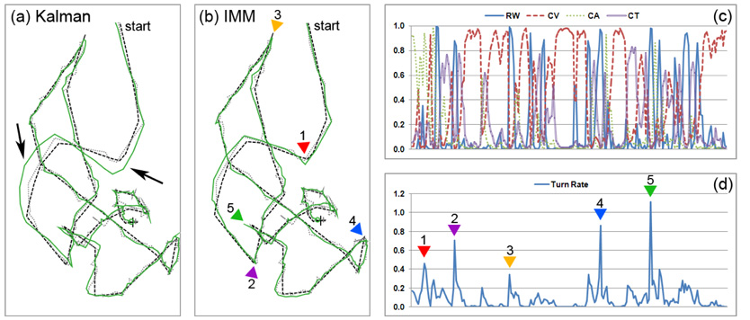
To illustrate the operation of the IMM filter (Section 3.4) and demonstrate its superiority to Kalman filter, an artificial example was devised as shown in Fig. 7. To reflect realistic cell motion and to serve as the ground truth, the trajectory of a cell in one of the sequences in dataset B was manually tracked. Gaussian noise of covariance 25I is added to the trajectory to simulate the measured cell positions during tracking, where I is a 2 × 2 identity matrix. The IMM filter with the four motion models described in Section 3.4.1, as well as a standard Kalman filter using only the constant-velocity (CV) model, is then executed to estimate the cell trajectory based on the noisy measurements. Both filters utilized equivalent parameter settings.

Fig. 7.

IMM filter versus Kalman filter. Black dashed curves in (a) and (b) represent the true trajectory of a cell. Gray dotted curves show the noisy trajectories after superimposing additive Gaussian noise. Solid green curves are the estimated trajectories by the Kalman and IMM filers using the noisy trajectories as measurements. Plots (c) and (d) show the model weights ${\rho }_k^j$ (j = 1,…,4) and the turn rates θ_k estimated by the IMM filter during its operation. Colored triangles in (b) and (d) indicate major turning points of the trajectory.

As shown in Fig. 7(a), the trajectory estimated by the Kalman filter (green curve) diverges from the true trajectory (black dashed curve) at the arrow-indicated positions, indicating that the CV model is no longer adequate to represent the turning motion at these locations. In comparison, the trajectory estimated by the IMM filter stays close to the ground truth, and exhibits appreciably smaller deviation from the true trajectory.

To provide additional insights into the IMM filter, we plotted the model weights ${\rho }_k^j$ (j = 1,…,4) (Fig. 7(c)) and the turn rate θ_k (Fig. 7(d)) estimated by the filter during its operation. As shown in these plots, the major turning points of the trajectory are indicated by peaks in the estimated turn rates, with higher peaks indicating tighter turns. An interesting exception is at the location indicated by triangle 3, where a near 180° turn is spotted in the trajectory, but the corresponding peak in the turn rate is relatively small. By examining the ground truth, we found that the cell stopped at the aforementioned location for a short period (approx. 20 minutes) before heading toward a different direction, resulting in a smaller turn rate. The stopping motion is captured by an increase in the random-walk model weight at the corresponding location in Fig. 7 (c).

The effect of spatiotemporal track linking is illustrated in Fig. 8. The top row of the figure shows the track segments, which are intermediate outputs of the track compiler. As shown, the trajectory of cell 1 and its daughters are broken in to multiple segments due to abrupt jumping motions of the cells. The bottom row shows the result after track linking, where the identities of the daughter cells and their lineage with cell 1 were successfully recovered.

Fig. 8.

Example of spatiotemporal track linking. Top: Track segments output by the track compiler. Bottom: Completed cell trajectories after track linking. The numbers in the parentheses indicate cell generations.

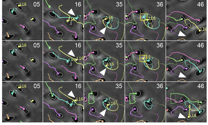
With the incorporation of IMM motion filter and spatiotemporal track linking (Section 3.6), our system achieves superior robustness in handling varying cell motions and long-term occlusions. Fig. 9 shows a 20×20-pixel portion of the tracking result for a sequence in dataset B. In this example, cell 116 is occluded by cell 47 in frame 36 and reappeared in frame 46. With a standard Kalman motion filter and no spatiotemporal linking, the system (top row) switched the identities of cells 47 and 116 in frame 16, detected a false mitosis in frame 36, and eventually lost cell 47 after frame 36. By replacing the Kalman filter with an IMM filter, the system correctly maintained the identities of cell 47 and 116, but it still lost track of cell 116 due to occlusion (middle row). Finally, by incorporating spatiotemporal optimization, the system correctly recovered the trajectory of cell 116 after occlusion (bottom row).

Fig. 9.

Tracking AE cells through occlusion. Cell 116 was completely occluded by cell 47 from frame 35 to 45 and reappeared in frame 46. The numbers at the top-right corner are frame indices. The trailing curves represent cell trajectories. Different colors represent different cell lineages. Top: With standard Kalman motion filter and no spatiotemporal track linking, the system switched the identities of cell 116 and cell 47 and loses track of cell 116 eventually. Middle: By replacing the Kalman filter with an IMM filter, the system correctly maintained the identities of cells 47 and 116. Bottom: By incorporating both IMM motion filter and spatiotemporal track linking, the system successfully tracked all cells.

5.2 Detection and Tracking Accuracy

The selected experimental datasets represent high and varying densities of cell populations as well as a variety of complex cell behaviors, which pose significant challenges for the tracking system. For example, the cell populations in datasets B and dataset C are nearly confluent towards the end of each sequence, with densities as high as approximately 30 cells per 100² pixels. In addition, while the typical diameter of AE stem cells in the experimental image sequence is around 5–12 pixels, some cells migrate more than 20 pixels between frames, which is a distance much larger than the cell diameter. The active contour tracker alone is insufficient to handle such large displacements. Moreover, some of the cells were frequently occluded in some frames and reemerged in other frames. Under these challenging conditions, our system achieved high detection and tracking accuracy as summarized in Table 2 and Table 3, respectively.

Table 2.

Summary of cell detection accuracy for all datasets.

Dataset	Cell Count	Detected	FP	FN	Precision (%)	Recall (%)
A	673	662	9	20	98.6	97.0
B	9879	9987	271	163	97.3	98.4
C	2126	2107	44	63	97.9	97.0
Overall	12678	12756	324	246	97.5	98.1

Table 3.

Summary of tracking validity and division tracking accuracy of the automated tracking results as compared with manual tracking.

	Tracking Validity
Sequences	Kalman		IMM		IMM + Track Linking
A1	70/81	(86.4%)	72/81	(88.9%)	75/81	(92.6%)
A2	82/93	(88.2%)	82/93	(88.2%)	86/93	(92.5%)
B1	70/92	(76.1%)	73/92	(79.3%)	81/92	(88.0%)
B2	90/117	(76.9%)	94/117	(80.3%)	101/117	(86.3%)
B3	81/104	(77.8%)	83/104	(79.8%)	91/104	(87.5%)
B4	80/108	(74.1%)	84/108	(77.8%)	93/108	(86.1%)
C1	98/121	(81.0%)	102/121	(84.3%)	110/121	(90.9%)
	Division Tracking Ratio
Sequences	Kalman		IMM		IMM + Track Linking
A1	1/1	(100%)	1/1	(100%)	1/1	(100%)
A2	0/0	(N/A)	0/0	(N/A)	0/0	(N/A)
B1	43/55	(78.2%)	43/55	(78.2%)	47/55	(85.5%)
B2	41/52	(78.8%)	42/52	(80.8%)	45/52	(86.5%)
B3	36/48	(75.0%)	37/48	(77.1%)	41/48	(85.4%)
B4	44/57	(77.2%)	47/57	(82.5%)	50/57	(87.7%)
C1	32/42	(76.2%)	33/42	(78.6%)	37/42	(88.1%)

The first column of Table 3 summarizes the tracking performance of our system with a standard Kalman motion filter and a constant-velocity motion model. The second column shows the performance with an adaptive IMM motion filter and four motion models as described in Section 3.4.1. The third column shows the performance after the incorporation of spatiotemporal track linking. As the statistics suggests, the incorporation of spatiotemporal track linking leads to significant performance boosts (as much as a 12% difference) compared to the Kalman filter-based system. In comparison, the IMM filter provides relative small performance improvements. However, the IMM filter still always outperforms the Kalman filter, and helps to resolve certain challenging tracking scenarios. One example is shown in Fig. 9. With the incorporation of IMM filter and spatiotemporal track linking, our system achieved overall tracking validity of 92.5% for dataset A, 86.9% for dataset B, and 90.9% for dataset C. It achieved overall division tracking ratios of 100% for dataset A, 86.3% for dataset B, and 88.1% for dataset C.

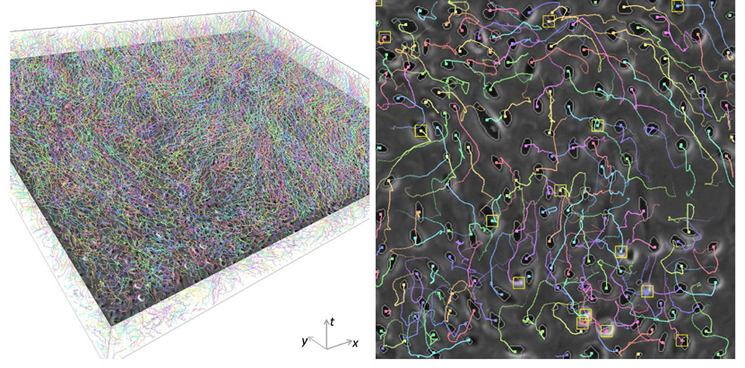
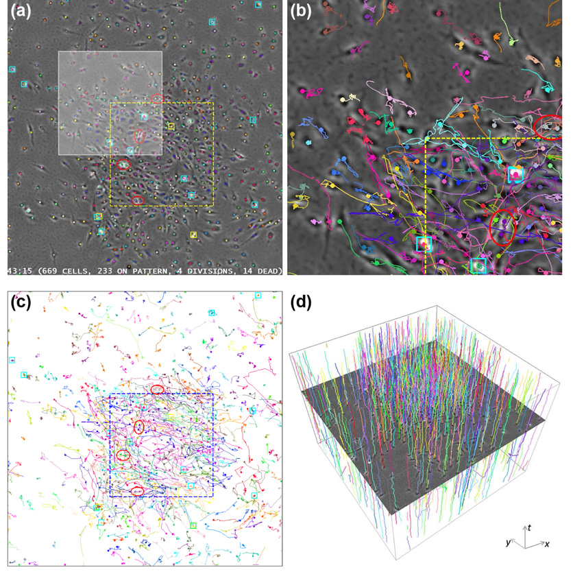
A visualization of the automatically tracked trajectories of more than 4000 AE stem cells across 256 frames is provided in Figure 10, and a visualization of the tracking result for MG-63 cells is shown in Figure 11.

Fig. 10.

Visualization of the tracking result of AE cells. Left: Spatiotemporal visualization of cell trajectories. Right: One of the selected regions used for quantitative validation with cell trajectories overlaid. Yellow rectangles indicate occurrences of mitosis in the past T = 10 frames.

Fig. 11.

Automatically-tracked MG-63 cell trajectories. The yellow and blue dashed lines indicate the location of the printed growth-factor pattern. Red ellipses indicate cell division. Cyan squares indicate dead cells. Yellow squares indicate mitotic or apoptotic cells. Cells inherit the colors of their farthest ancestors. (a) A sample frame with cell centroids overlaid. (b) Magnified view of the highlighted region in (a) with automatically tracked cell trajectories overlaid. (c) and (d) 2-D and spatiotemporal rendering of the automatically tracked cell trajectories.

5.3 Lineage Construction

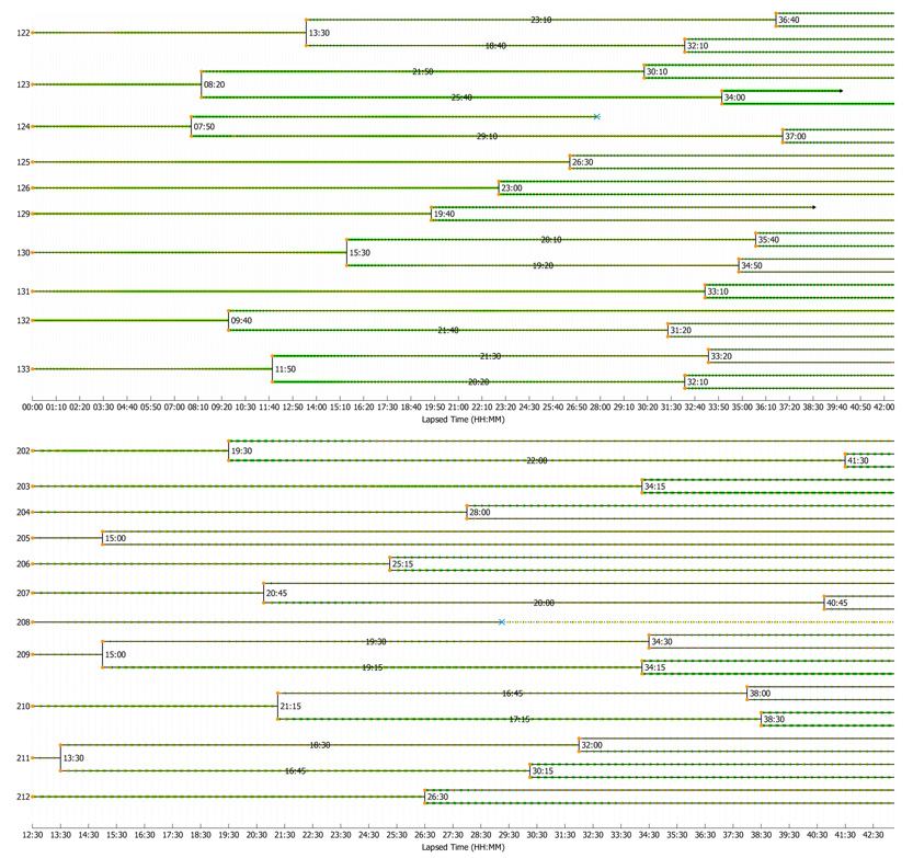
One application of the tracking system is to automatically reconstruct cell lineage maps, which is especially important for stem cell research. In addition to revealing the mother-daughter relations between cells, metrics such as symmetry and division times can also be derived from lineage maps. Symmetry, which is defined as the mitotic fraction, is a measure of the capability of a stem cell to divide and produce daughter cells that are essentially identical to the mother, thus representing self-renewal (Deasy and Huard, 2002). And, the division time, which is defined as the lapsed time between cytokinetic events, is a key parameter in determining the expansion rate of stem cell populations. For example, these metrics can be used in predictive models of stem cell population growth during cell culture expansions (Deasy and Huard, 2002), as well as the design and optimization of subculturing strategies.

We utilized the system to construct the lineage maps for the entire populations of AE stem cells in dataset B and of MG-63 cells in dataset C. Our system correctly constructed 62.4% of the lineage trees for AE stem cells and 68.3% for MG-63 cells as measured in the selected regions of interest (see Section 3.4); Fig. 12 shows samples of the correctly constructed lineage trees with cells undergoing multiple divisions. In general, achieving higher accuracy is challenging since a single tracking error will invalidate the entire lineage tree that the cell belongs to. However, alternative approaches for mitosis/apoptosis event detection (Li et al., 2008) and spatiotemporal image processing techniques (Padfield et al., 2006a) could potentially improve lineage tracking accuracy. Increasing the image acquisition rate would be another possibility to reduce ambiguities and hence increase tracking accuracy. We also emphasize that acceptable accuracy levels required in various experiments, using large and dense cell populations, will likely vary depending on the specific biological question being proposed.

Fig. 12.

Portions of color-coded lineage maps of AE cells (top) and MG-63 cells (bottom) constructed based on automated tracking results. Green line segments indicate the relative migration distances, where a longer line segment suggests a longer migration distance up to the current time point. Black arrows indicate cell departure. Blue crosses indicate cell death. Texts on the lineage lines show the division times.

5.4 Computation Time

All of the above experiments were conducted on a computer with a 2.66 GHz Intel Xeon processor and 4 GB memory, running 64-bit Gentoo Linux operating system. Our system runs at an average speed of 90 frames/hour for tracking approximately 3000 cells in a 1280×1024 pixels/frame image sequence. The most time consuming computation step is the level set evolution.

6 Conclusion

We developed and validated an automated system capable of simultaneously tracking thousands of individual cells in dense cell populations in phase contrast microscopy image sequences. The system employs a modular design, which integrates an efficient cell detector, a topology-constrained geometric active contour tracker, a biologically relevant IMM motion filter, and spatiotemporal trajectory optimization. Our system enables automatic quantification of cell migration, proliferation, apoptosis, and construction of cell lineage maps, which facilitates the analysis of massive biological datasets. For future work, we will focus on further improving tracking accuracy for automated cell lineage construction, and applying the system to tackle challenging biological problems.

A Two-Cycle Fast Level Set Algorithm

Algorithm 4 provides the pseudocode of the fast dual-cycle level set algorithm described in Section 3.3.3. Figure A.1 illustrates the key steps of the algorithm. The input to the algorithm is the region labeling map ψ_k−1(x, y) for frame k − 1; the output is the evolved labeling map ψ̂_k(x, y) for frame k. There are three parameters: the maximum iterations of the main loop (T_max), the

Algorithm 4.

Fast Dual-Cycle Level Set Evolution

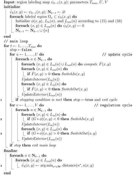number of iterations for the update cycle (U), and the number of iterations for the regulation cycle (V). U and V controls the relative strength of regulation, which replace the parameter ν in Equation (11). We set T_max = 500, U = 3, and V = 1 in all the experiments.

Fig. A.1.

Illustration of fast level set initialization, evolution, and finalization.

The stopping condition (Line 1) is satisfied if F(x, y) ≤ 0, ∀ (x, y) ∈ L_out(n), ∀n and F(x, y) ≥ 0, ∀(x, y) ∈ L_in(n), ∀n. The discrete Gaussian kernel G (Lines 2 and 3) is approximated by:

$$G=\left[\begin{array}{ccc}1& 2& 1\\ 2& 4& 2\\ 1& 2& 1\end{array}\right].$$ (A.1)

N* (Line 4) denotes the set {n ∈ N_k−1|Ω_n ∩ N₄(x, y) ≠ Ø}, and the distance function is defined as:

$$\text{distance}(n^{*},n|x,y)=|I_k(x^{*},y^{*})-I_k(x,y)|,$$

where (x^*, y^*) ∈ N₄(x, y), ψ(x, y) = n^*, and ψ(x, y) = n.

The psuedocode of the procedures SwitchIn, UpdateInterior, SwitchOut, and UpdateExterior, which are required by the dual-cycle algorithm, are listed in Algorithm 5, Algorithm 6, Algorithm 7, and Algorithm 8.

Algorithm 5.

Procedure SwitchIn

Algorithm 6.

Procedure UpdateInterior

Algorithm 7.

Procedure SwitchOut

Algorithm 8.

Procedure UpdateExterior

B EM-IMM Parameter Estimation

The unknown parameters are denoted by Θ ≡ {Qⁱ, R, ${\mathrm{\Sigma }}_0^i$}. Our objective is to estimate the parameters Θ and the hidden states S = {s₀,…,s_K} based on the measurements Z = {z₋₂,…,z_K}. We make the index of the measurement sequence to start from −2 for the convenience of notation. The initial state s₀ is obtained using the first three measurements {z₋₂, z₋₁, z₀}.

The EM algorithm maximizes the complete-data log likelihood, defined by

$$\begin{array}{cc}\text{log}P(\mathbf{S},\mathbf{Z}|\mathbf{\Theta })=\hfill & -\frac{K}{2}\text{log}|{\mathbf{Q}}^i|-\frac{K}{2}\text{log}|\mathbf{R}|-\frac{1}{2}\text{log}|{\mathrm{\Sigma }}_0^i|\hfill \\ \hfill & -\frac{1}{2}{\displaystyle \sum _{k=1}^K({\mathbf{z}}_k-\mathbf{H}{\mathbf{s}}_k{)}^{\prime }}{\mathbf{R}}^{-1}({\mathbf{z}}_k-\mathbf{H}{\mathbf{s}}_k)\hfill \\ \hfill & -\frac{1}{2}{\displaystyle \sum _{k=1}^K({\mathbf{s}}_k-{\mathbf{F}}^i{\mathbf{s}}_{k-1}{)}^{\prime }}{({\mathbf{Q}}^i)}^{-1}({\mathbf{s}}_k-{\mathbf{F}}^i{\mathbf{s}}_{k-1})+\text{constant},\hfill \end{array}$$ (B.1)

where |·| denotes matrix determinant. The maximization of log P(S,Z|Θ) with respect to the unknown parameters Θ is a chicken-and-egg problem since the system states S are also unknown. The EM algorithm solves this problem by iterating between two steps: expectation (E) and maximization (M).

B.1 E Step

The E step finds the expected value of the complete-data log likelihood with respect to the unknown states S, given the observed data Z and the current parameter estimates Θ^old:

$$𝒬(\mathbf{\Theta }|{\mathbf{\Theta }}^{\text{old}})=E[\text{log}P(\mathbf{S},\mathbf{Z},\mathbf{\Theta }|\mathbf{Z},{\mathbf{\Theta }}^{\text{old}})].$$ (B.2)

This quantity depends on three expectations:

$${\widehat{\mathbf{s}}}_{k|K}\equiv E\left[{\mathbf{s}}_k|\mathbf{Z},{\mathbf{\Theta }}^{\text{old}})\right]$$ (B.3)

$${\mathrm{\Sigma }}_{k|K}\equiv E\left[{\mathbf{s}}_k{\mathbf{s}}_k^{\prime }|\mathbf{Z},{\mathbf{\Theta }}^{\text{old}})\right]$$ (B.4)

$${\mathrm{\Sigma }}_{k,k-1|K}\equiv E\left[{\mathbf{s}}_k{\mathbf{s}}_{k-1}^{\prime }|\mathbf{Z},{\mathbf{\Theta }}^{\text{old}})\right]$$ (B.5)

Note that the estimates ŝ_k|K and Σ̂_k|K differ from the ones computed by the forward-time IMM filter in that they depend on past as well as future observations. To obtain these estimates, the fixed-interval IMM smoother in (Helmick et al., 1995) is utilized. The algorithm uses two IMM filters. One of the filters propagates in the forward-time direction, and produces estimates ${\widehat{\mathbf{s}}}_k^j$ and ${\mathrm{\Sigma }}_k^j$ as given previously. The other filter propagates in the backward-time direction, and produces estimates ${\widehat{\mathbf{s}}}_k^{b,i},{\mathrm{\Sigma }}_k^{b,i},{\widehat{\mathbf{s}}}_{k|k+1}^{b,i}\text{and}{\mathrm{\Sigma }}_{k|k+1}^{b,i}$. We refer the reader to (Helmick et al., 1995) for details on the backward-time IMM filter. The fixed-interval IMM smoother combines the forward and backward filtered outputs to obtain smoothed estimates according to the following procedure.

Step 1

Compute combined estimates:

$$\begin{array}{cc}\hfill {\widehat{\mathbf{s}}}_{k|K}^{ji}& ={\mathrm{\Sigma }}_{k|K}^{ji}[{({\mathrm{\Sigma }}_k^j)}^{-1}{\widehat{\mathbf{s}}}_k^j+{({\mathrm{\Sigma }}_{k|k+1}^{b,i})}^{-1}{\widehat{\mathbf{s}}}_{k|k+1}^{b,i})],\hfill \\ \hfill {\mathrm{\Sigma }}_{k|K}^{ji}& ={\left[{({\mathrm{\Sigma }}_k^j)}^{-1}+{({\mathrm{\Sigma }}_{k|k+1}^{b,i})}^{-1}\right]}^{-1},\hfill \\ \hfill {\mathrm{\Sigma }}_{k+1,k|K}^{ji}& ={\left[{({\mathrm{\Sigma }}_{k+1,k|k}^j)}^{-1}+{({\mathrm{\Sigma }}_{k+1,k|k+1}^{b,i})}^{-1}\right]}^{-1},\hfill \end{array}$$ (B.6)

with ${\mathrm{\Sigma }}_{k+1,k|k}^j={\mathbf{F}}^j{\mathrm{\Sigma }}_k^j,\text{and}{\mathrm{\Sigma }}_{k+1,k|k+1}^{b,i}={\mathrm{\Sigma }}_{k+1}^{b,i}[{({\mathbf{F}}^i)}^{-1}{]}^{\prime }.$

Step 2

Compute model-conditioned smoothed estimates:

$$\begin{array}{cc}\hfill {\widehat{\mathbf{s}}}_{k|K}^j& ={\displaystyle \sum _{i=1}^r{\rho }_{k+1|K}^{i|j}{\widehat{\mathbf{s}}}_{k|K}^{ji},}\hfill \\ \hfill {\mathrm{\Sigma }}_{k|K}^j& ={\displaystyle \sum _{i=1}^r{\rho }_{k+1|K}^{i|j}}\left[{\mathrm{\Sigma }}_{k|K}^{ji}+({\widehat{\mathbf{s}}}_{k|K}^{ji}-{\widehat{\mathbf{s}}}_{k|K}^j)({\widehat{\mathbf{s}}}_{k|K}^{ji}-{\widehat{\mathbf{s}}}_{k|K}^j{)}^{\prime }\right],\hfill \\ \hfill {\mathrm{\Sigma }}_{k+1,k|K}^j& ={\displaystyle \sum _{i=1}^r{\rho }_{k+1|K}^{i|j}}\left[{\mathrm{\Sigma }}_{k+1,k|K}^{ji}+({\widehat{\mathbf{s}}}_{k+1|K}^{ji}-{\widehat{\mathbf{s}}}_{k+1|K}^j)({\widehat{\mathbf{s}}}_{k|K}^{ji}-{\widehat{\mathbf{s}}}_{k|K}^j{)}^{\prime }\right].\hfill \end{array}$$ (B.7)

The conditional probability ${\rho }_{k+1|K}^{i|j}$ is obtained by

$${\rho }_{k+1|K}^{i|j}=p_{ij}{\lambda }_k^{ji}/{\gamma }_j,\text{with}{\gamma }_j={\displaystyle \sum _{i=1}^r{p}_{ji}{\lambda }_k^{ji}.}$$ (B.8)

The likelihood ${\lambda }_k^{ji}$ is given by

$${\lambda }_k^{ji}=𝒩({\widehat{\mathbf{s}}}_{k|k+1}^{b,i}-{\widehat{\mathbf{s}}}_k^j;0,{\mathrm{\Sigma }}_{k|k+1}^{b,i}+{\mathrm{\Sigma }}_k^j),$$ (B.9)

where 𝒩(·) denotes a multivariate normal distribution.

Step 3

Compute the overall smoothed estimates:

$$\begin{array}{cc}\hfill {\widehat{\mathbf{s}}}_{k|K}& ={\displaystyle \sum _{j=1}^r{\rho }_k^{s,j}{\widehat{\mathbf{s}}}_{k|K}^j,}\hfill \\ \hfill {\mathrm{\Sigma }}_{k|K}& ={\displaystyle \sum _{j=1}^r{\rho }_k^{s,j}}\left[{\mathrm{\Sigma }}_{k|K}^j+({\widehat{\mathbf{s}}}_{k|K}^j-{\widehat{\mathbf{s}}}_{k|K})({\widehat{\mathbf{s}}}_{k|K}^j-{\widehat{\mathbf{s}}}_{k|K}{)}^{\prime }\right],\hfill \\ \hfill {\mathrm{\Sigma }}_{k+1,k|K}& ={\displaystyle \sum _{j=1}^r{\rho }_k^{s,j}}\left[{\mathrm{\Sigma }}_{k+1,k|K}^j+({\widehat{\mathbf{s}}}_{k+1|K}^j-{\widehat{\mathbf{s}}}_{k+1|K})({\widehat{\mathbf{s}}}_{k|K}^j-{\widehat{\mathbf{s}}}_{k|K}{)}^{\prime }\right].\hfill \end{array}$$ (B.10)

The smoothed model probability ρ^s,j can be computed as

$${\rho }_k^{s,j}=\frac{{\gamma }_j{\rho }_k^j}{{\displaystyle {\sum }_{j=1}^r{\gamma }_j{\rho }_k^j}},$$ (B.11)

where ${\rho }_k^j$ is the forward-time filtered model probability.

B.2 M Step

The M-step of the EM algorithm re-estimates the unknown parameters by maximizing the expectation computed in the first step, i.e.,

$${\mathbf{\Theta }}^{\text{new}}=\underset{\mathbf{\Theta }}{\text{max}}𝒬(\mathbf{\Theta }|{\mathbf{\Theta }}^{\text{old}}).$$ (B.12)

By taking the partial derivatives of 𝒬 with respect to (Qⁱ)⁻¹ and R⁻¹, and setting the respective result to zero, we obtain

$$\begin{array}{cc}{({\mathbf{Q}}^i)}^{\text{new}}=\hfill & \frac{1}{K}{\displaystyle \sum _{k=1}^K[{\mathrm{\Sigma }}_{k|K}-{\mathbf{F}}^i{\mathrm{\Sigma }}_{k-1,k|K}}\hfill \\ \hfill & -{\mathrm{\Sigma }}_{k,k-1|K}({\mathbf{F}}^i{)}^{\prime }+{\mathbf{F}}^i{\mathrm{\Sigma }}_{k-1|K}({\mathbf{F}}^i{)}^{\prime }],\hfill \end{array}$$ (B.13)

$${\mathbf{R}}^{\text{new}}=\frac{1}{K}{\displaystyle \sum _{k=1}^K\left({\mathbf{z}}_k{\mathbf{z}}_k^{\prime }-2\mathbf{H}{\widehat{\mathbf{s}}}_{k|K}{\mathbf{z}}_k^{\prime }+\mathbf{H}{\mathrm{\Sigma }}_{k|K}\mathbf{H\prime }\right),}$$ (B.14)

$${({\mathrm{\Sigma }}_0^i)}^{\text{new}}={\mathrm{\Sigma }}_{0|K}.$$ (B.15)

The expectation and maximization steps are computed repeatedly until the relative absolute change of the expected log likelihood is below a threshold. Each iteration is guaranteed to increase the log likelihood, and the algorithm will converge to a local maximum of the log likelihood function.

References

- Al-Kofahi O, Radke RJ, Goderie SK, Shen Q, Temple S, Roysam B. Automated cell lineage construction: A rapid method to analyze clonal development established with murine neural progenitor cells. Cell Cycle. 2006 Feb;5(3):327–335. doi: 10.4161/cc.5.3.2426. [DOI] [PubMed] [Google Scholar]
- Appel K, Haken W. Every planar map is four colorable, Part I: Discharging. Illinois J. Math. 1977a;21:429–490. [Google Scholar]
- Appel K, Haken W. Every planar map is four colorable, Part II: Reducibility. Illinois J. Math. 1977b;21:491–567. [Google Scholar]
- Bahnson A, Athanassiou C, Koebler D, Qian L, Shun T, Shields D, Yu H, Wang H, Goff J, Cheng T, Houck R, Cowsert L. Automated measurement of cell motility and proliferation. BMC Cell Biology. 2005 Apr;6(19) doi: 10.1186/1471-2121-6-19. [DOI] [PMC free article] [PubMed] [Google Scholar]
- Bao Z, Murray JI, Boyle T, Ooi SL, Sandel MJ, Waterston RH. Automated cell lineage tracing in caenorhabditis elegans. Proceedings of the National Academy of Sciences. 2006 Feb;103(8):2707–2712. doi: 10.1073/pnas.0511111103. [DOI] [PMC free article] [PubMed] [Google Scholar]
- Berkelaar M, Dirks J, Eikland K, Notebaert P. lpsolve: A mixed integer linear programming (MILP) solver. 2007 URL http://sourceforge.net/projects/lpsolve.
- Bishop CM. Pattern Recognition and Machine Learning. Springer; 2007. [Google Scholar]
- Blom HAP. An efficient filter for abruptly changing systems; Proc. 23rd IEEE Conference on Decision and Control; 1984. Dec, pp. 656–658. [Google Scholar]
- Braun V, Azevedo RBR, Gumbel1 M, Agapow P-M, Leroi AM, Meinzer H-P. ALES: Cell lineage analysis and mapping of developmental events. Bioinformatics. 2003;19(7):851–858. doi: 10.1093/bioinformatics/btg087. [DOI] [PubMed] [Google Scholar]
- Brox T, Weickert J. Level set segmentation with multiple-regions. IEEE Trans. Image Processing. 2006;15(10):3213–3218. doi: 10.1109/tip.2006.877481. [DOI] [PubMed] [Google Scholar]
- Bunyak F, Palaniappan K, Nath SK, Baskin TI, Dong G. Quantitative cell motility for in vitro wound healing using level set-based active contour tracking; Proc. 3rd IEEE Int. Symp. Biomed. Imaging (ISBI); 2006. Apr, pp. 1040–1043. [DOI] [PMC free article] [PubMed] [Google Scholar]
- Campbell PG, Miller ED, Fisher GW, Walker LM, Weiss LE. Engineered spatial patterns of FGF-2 immobilized on fibrin direct cell organization. Biomaterials. 2005 Nov;26:6762–6770. doi: 10.1016/j.biomaterials.2005.04.032. [DOI] [PubMed] [Google Scholar]
- Canny J. A computational approach to edge detection. IEEE Trans. Pattern Anal. Machine Intell. 1986 Nov;8:679–698. [PubMed] [Google Scholar]
- Caselles V, Kimmel R, Sapiro G. Geodesic active contours. Int. J. Computer Vision. 1997;22(1):61–79. [Google Scholar]
- Cates JE, Lefohn AE, Whitaker RT. GIST: An interactive, GPU-based level set segmentation tool for 3D medical images. Medical Image Analysis. 2004 Sep;8:217–231. doi: 10.1016/j.media.2004.06.022. [DOI] [PubMed] [Google Scholar]
- Cheng Y. Mean shift, mode seeking, and clustering. IEEE Trans. Pattern Anal. Machine Intell. 1995 Aug;17(8):790–799. [Google Scholar]
- Chopp DL. Computing minimal surfaces via level set curvature flow. Journal of Computational Physics. 1993 May;106:77–91. [Google Scholar]
- Cremers D, Rousson M, Deriche R. A review of statistical approaches level set segmentation: Integrating color, texture, motion and shape. Int. J. Computer Vision. 2007;72(2):195–215. [Google Scholar]
- Deasy B, Huard J. Gene therapy and tissue engineering based on muscle-derived stem cells. Current Opinion in Molecular Therapeutics. 2002;4:382–389. [PubMed] [Google Scholar]
- Debeir O, Ham PV, Kiss R, Decaestecker C. Tracking of migrating cells under phase-contrast video microscopy with combined mean-shift processes. IEEE Trans. Med. Imag. 2005 Jun;24:697–711. doi: 10.1109/TMI.2005.846851. [DOI] [PubMed] [Google Scholar]
- Doucet A, Ristic B. Recursive state estimation for multiple switching models with unknown transition probabilities. IEEE Trans. Aerosp. Electron. Syst. 2002 Jul;38(3):1098–1104. [Google Scholar]
- Dufour A, Shinin V, Tajbakhsh S, Guillen-Aghion N, Olivo-Marin J-C, Zimmer C. Segmenting and tracking fluorescent cells in dynamic 3-d microscopy with coupled active surfaces. IEEE Trans. Image Processing. 2005 Sep;14(9):1396–1410. doi: 10.1109/tip.2005.852790. [DOI] [PubMed] [Google Scholar]
- Feng H, Castanon DA, Karl WC. A curve evolution approach for image segmentation using adaptive flows; Proc. IEEE Int. Conf. Comp. Vision; 2001. Jul, pp. 494–499. [Google Scholar]
- Genovesio A, Liedl T, Emiliani V, Parak WJ, Coppey-Moisan M, Olivo-Marin J-C. Multiple particle tracking in 3-D+t microscopy: Method and application to the tracking of endocytosed quantum dots. IEEE Trans. Image Processing. 2006 May;15(5):1062–1070. doi: 10.1109/tip.2006.872323. [DOI] [PubMed] [Google Scholar]
- Godinez WJ, Lampe M, Worz S, Muller B, Eils R, Rohr K. Tracking of virus particles in time-lapse fluorescence microscopy image sequences; Proc. IEEE Int’l. Symp. Biomed. Imaging; 2007. Apr, pp. 256–259. [DOI] [PubMed] [Google Scholar]
- Goldenberg R, Kimmel R, Rivlin E, Rudzsky M. Fast geodesic active contours. IEEE Trans. Med. Imag. 2001 Oct;10(10):1467–1475. doi: 10.1109/83.951533. [DOI] [PubMed] [Google Scholar]
- Gordon NJ, Salmond DJ, Smith AFM. Novel approach to nonlinear/non-Gaussian Bayesian state estimation; IEE Proceedings-F; 1993. Apr, pp. 107–113. [Google Scholar]
- Han X, Xu C, Prince JL. A topology preserving level set method for geometric deformable models. IEEE Trans. Pattern Anal. Machine Intell. 2003 Jun;25(6):755–768. [Google Scholar]
- Helmick RE, Blair WD, Hoffman SA. Fixed-interval smoothing for Markovian switching systems. IEEE Trans. Inform. Theory. 1995 Nov;41(6):1845–1855. [Google Scholar]
- Herman SM. Ph.D. thesis. 2002. A particle filtering approach to joint passive radar tracking and target classification. [Google Scholar]
- Huang S, Law P, Francis K, Palsson BO, Ho AD. Symmetry of initial cell divisions among primitive hematopoietic progenitors is independent of ontogenic age and regulatory molecules. Blood. 1999 Oct;94(8):2595–2604. [PubMed] [Google Scholar]
- Huang X, Metaxas D, Chen T. Metamorphs: Deformable shape and texture models; Proc. IEEE Computer Society Conference on Computer Vision and Pattern Recognition (CVPR); 2004. Jun, pp. 496–503. [Google Scholar]
- Jilkov VP, Li XR. Online Bayesian estimation of transition probabilities for Markovian jump systems. IEEE Trans. Signal Processing. 2004 Jun;52(6):1620–1630. [Google Scholar]
- Kalman, Rudolph E. A new approach to linear filtering and prediction problems. Transactions of the ASME - Journal of Basic Engineering. 1960;82(Series D):35–45. [Google Scholar]
- Kanade T, Li K. Tracking of migrating and proliferating cells in phase-contrast microscopy imagery for tissue engineering; Proc. Computer Vision for Biomedical Image Applications Workshop; 2005. Oct, p. 24. [Google Scholar]
- Kirubarajan T, Bar-Shalom Y, Pattipati KR. Multiassignment for tracking a large number of overlapping objects [and application to fibroblast cells] IEEE Trans. Aerosp. Electron. Syst. 2001 Jan;37(1):2–21. [Google Scholar]
- Lefohn A, Kniss J, Hansen C, Whitaker R. A streaming narrowband algorithm: Interactive computation and visualization of level sets. IEEE Trans. Visual. Comput. Graphics. 2004 Jul;10:422–433. doi: 10.1109/TVCG.2004.2. [DOI] [PubMed] [Google Scholar]
- Li K, Chen M, Kanade T. Proc. Medical Image Computing and Comp.-Assisted Intervention. Springer; 2007. Oct, Cell population tracking and lineage construction with spatiotemporal context. in press. [DOI] [PubMed] [Google Scholar]
- Li K, Kanade T, Chen M, Miller ED, Weiss LE, Campbell PG. Computer vision tracking of stemness; Proc. IEEE Int’l. Symp. Biomed. Imaging; 2008. May, In press. [Google Scholar]
- Li K, Miller ED, Weiss LE, Campbell PG, Kanade T. Online tracking of migrating and proliferating cells imaged with phase-contrast microscopy; Proc. IEEE Conf. Comp. Vision and Patt. Recog. Workshop; 2006. Jun, pp. 65–72. [Google Scholar]
- Mansouri A-R, Mitiche A, Vazquez C. Multiregion competition: A level set extension of region competition to multiple region image partitioning. Computer Vision and Image Understanding. 2006;101:137–150. [Google Scholar]
- Meyer F. A threshold selection method from gray level histograms. The Journal of Histochemistry and Cytochemistry. 1979;27(1):128–135. doi: 10.1177/27.1.438499. [DOI] [PubMed] [Google Scholar]
- Miki T, Lehmann T, Cai H, Stolz DB, Strom SC. Stem cell characteristics of amniotic epithelial cells. Stem Cells. 2005 Aug; doi: 10.1634/stemcells.2004-0357. [DOI] [PubMed] [Google Scholar]
- Miller ED, Fisher GW, Weiss LE, Walker LM, Campbell PG. Dose-dependent cell growth in response to concentration modulated patterns of FGF-2 printed on fibrin. Biomaterials. 2006 Apr;27:2213–2221. doi: 10.1016/j.biomaterials.2005.10.021. [DOI] [PubMed] [Google Scholar]
- Mukherjee DP, Ray N, Acton ST. Level set analysis for leukocyte detection and tracking. IEEE Trans. Image Processing. 2004 Apr;13:562–572. doi: 10.1109/tip.2003.819858. [DOI] [PubMed] [Google Scholar]
- Nath S, Palaniappan K, Bunyak F. Wound cell segmentation using coupled level sets and graph-vertex coloring; Proc. Medical Image Computing and Comp.-Assisted Intervention; 2006. Oct, pp. 101–108. [DOI] [PMC free article] [PubMed] [Google Scholar]
- Osher S, Sethian JA. Fronts propagating with curvature dependent speed: Algorithms based on Hamilton-Jacobi formulations. Jour. Comp. Phys. 1988;79:12–49. [Google Scholar]
- Otsu N. A threshold selection method from gray level histograms. IEEE Trans. Syst., Man, Cybern. 1979 Mar;9:62–66. [Google Scholar]
- Padfield D, Rittscher J, Roysam B. Spatio-temporal cell segmentation and tracking for automated screening; Proc. IEEE Int’l. Symp. Biomed. Imaging; 2008. May, In press. [Google Scholar]
- Padfield D, Rittscher J, Sebastian T, Thomas N, Roysam B. Spatio-temporal cell cycle analysis using 3D level set segmentation of unstained nuclei in line scan confocal fluorescence images; Proc. IEEE Int’l. Symp. Biomed. Imaging; 2006a. Apr, pp. 1036–1039. [Google Scholar]
- Padfield D, Rittscher J, Thomas N, Roysam B. Spatiotemporal cell cycle phase analysis using level sets and fast marching methods; Proc. Workshop on Microscopic Image Analysis with Applications in Biology; 2006b. Sep, pp. 2–9. URL http://www.miaab.org/miaab-2006-papers.html. [Google Scholar]
- Pan Y, Birdwell JD, Djouadi SM. Efficient implementation of the Chan-Vese models without solving PDEs; Proc. IEEE Int. Workshop Multimedia Sig. Proc; 2006. Oct, In press. [Google Scholar]
- Papadimitriou CH, Steiglitz K. Combinatorial Optimization: Algorithms and Complexity. Dover Publications; 1998. Jan, [Google Scholar]
- Patrick CW, Wu X. Integrin-mediated preadipocyte adhesion and migration on laminin-1. Annals of Biomedical Engineering. 2003;31:505–514. doi: 10.1114/1.1566446. [DOI] [PubMed] [Google Scholar]
- Perona P, Malik J. Scale-space and edge detection using anisotropic diffusion. IEEE Trans. Pattern Anal. Machine Intell. 1990 Jul;12(7):629–639. [Google Scholar]
- Phillippia JA, Miller ED, Weiss LE, Huard J, Waggoner AS, Campbell PG. Microenvironments engineered by inkjet bioprinting spatially direct adult stem cells toward muscle- and bone-like subpopulations. Stem Cells. 2008 Jan;26(1):127–134. doi: 10.1634/stemcells.2007-0520. [DOI] [PubMed] [Google Scholar]
- Ristic B, Arulampalam S, Gordon NJ. Beyond the Kalman Filter: Particle Filters for Tracking Applications. Artech House Publishers; 2004. Feb, [Google Scholar]
- Ségonne F. Ph.D. thesis. 2005. Dec, Segmentation of medical images under topological constraints. [Google Scholar]
- Sethian JA, editor. Level Set Methods and Fast Marching Methods: Evolving Interfaces in Computational Geometry, Fluid Mechanics, Computer Vision, and Materials Science. 2nd Edition. Cambridge University Press; 1999. Jan, [Google Scholar]
- Shi Y, Karl WC. A fast level set method without solving PDEs. Proc. IEEE Int. Conf. Acou. Speech and Signal Proc.; Philadelphia, PA. 2005a. Mar, pp. 97–100. [Google Scholar]
- Shi Y, Karl WC. Real-time tracking using level sets; Proc. IEEE Conf. Comp. Vision and Patt. Recog; 2005b. Jun, pp. 34–41. [Google Scholar]
- Smal I, Draegestein K, Galjart N, Niessen W, Meijering E. Rao-blackwellized marginal particle filtering for multiple object tracking in molecular bioimaging; Proc. Int’l. Conf. Information Processing in Medical Imaging; 2007. Jul, pp. 110–121. [DOI] [PubMed] [Google Scholar]
- Smal I, Niessen W, Meijering E. Bayesian tracking for fluorescence microscopic imaging; Proc. IEEE Int’l. Symp. Biomed. Imaging; 2006. Apr, pp. 550–553. [Google Scholar]
- Smith AFM, Makov UE. A quasi-Bayes sequential procedure for mixtures. Journal of the Royal Statistical Society, Series B. 1978;40(1):106–112. [Google Scholar]
- Sternberg S. Biomedical image processing. IEEE Computer. 1983 Jan;16(1):22–34. [Google Scholar]
- Vincent L, Soille P. Watersheds in digital spaces: An efficient algorithm based on immersion simulations. IEEE Trans. Pattern Anal. Machine Intell. 1991 Jun;13(6):583–598. [Google Scholar]
- Weiss LE, Amon C, Finger S, Miller E, Romero D, Verdinelli I, Walker L, Campbell P. Bayesian computer-aided experimental design of heterogeneous scaffolds for tissue engineering. Computer Aided Design. 2005;37:1127–1139. [Google Scholar]
- Yang F, Mackey MA, Ianzini F, Gallardo G, Sonka M. Cell segmentation, tracking, and mitosis detection using temporal context. In: Duncan JS, Gerig G, editors. Proc. Medical Image Computing and Comp.-Assisted Intervention; 2005a. Oct, pp. 302–309. [DOI] [PubMed] [Google Scholar]
- Yang X, Li H, Zhou X, Wong S. Automated segmentation and tracking of cells in time-lapse microscopy using watershed and mean shift; Proc. Int’l. Symp. Intelligent Signal Processing and Communication Systems; 2005b. Dec, pp. 533–536. [Google Scholar]
- Zarchan P, Musoff H. Fundamentals of Kalman Filtering: A Practical Approach. 2nd Edition. American Institute of Aeronautics and Astronautics, Inc.; 2005. [Google Scholar]
- Zhang B, Zimmer C, Olivo-Marin J-C. Tracking fluorescent cells with coupled geometric active contours. Proc. 2nd IEEE Int. Symp. Biomed. Imaging (ISBI); Arlington, VA. 2004. pp. 476–479. [Google Scholar]
- Zhu SC, Yuille A. Region competition: Unifying snakes, region growing, and Bayes/MDL for multiband image segmentation. IEEE Trans. Pattern Anal. Machine Intell. 1996 Sep;18(9):884–900. [Google Scholar]
- Zimmer C, Labruy‘ere E, Meas-Yedid V, Guill’en N, Olivo-Marin J-C. Segmentation and tracking of migrating cells in videomicroscopy with parametric active contours: A tool for cell-based drug testing. IEEE Trans. Med. Imag. 2002 Oct;21(10):1212–1221. doi: 10.1109/TMI.2002.806292. [DOI] [PubMed] [Google Scholar]
- Zimmer C, Olivo-Marin J-C. Coupled parametric active contours. IEEE Trans. Pattern Anal. Machine Intell. 2005 Nov;27(11):1838–1842. doi: 10.1109/TPAMI.2005.214. [DOI] [PubMed] [Google Scholar]