

Abstract
Given a set of alternative models for a specific protein sequence, the model quality assessment (MQA) problem asks for an assignment of scores to each model in the set. A good MQA program assigns these scores such that they correlate well with real quality of the models, ideally scoring best that model which is closest to the true structure.
In this paper, we present a new approach for addressing the MQA problem. It is based on distance constraints extracted from alignments to templates of known structure, and is implemented in the Undertaker [9] program for protein structure prediction. One novel feature is that we extract non-contact constraints as well as contact constraints.
We describe how the distance constraint extraction is done and we show how they can be used to address the MQA problem. We have compared our method on CASP7 targets and the results show that our method is at least comparable with the best MQA methods that were assessed at CASP7 [7].
We also propose a new evaluation measure, Kendall's τ, that is more interpretable than conventional measures used for evaluating MQA methods (Pearson's r and Spearman's ρ).
We show clear examples where Kendall's τ agrees much more with our intuition of a correct MQA and we therefore propose that Kendall's τ be used for future CASP MQA assessments.
2 Introduction
Most search algorithms for protein structure prediction are guided by cost functions that assess how “protein-like” particular conformations of the polypeptide chain are. In theory, a perfect cost function would guide a good search algorithm to the native state of the protein, but such a cost function has yet to be discovered.
One of the obstacles is that many low-cost structures usually exist in the conformational search space and even good cost functions have trouble identifying the most native-like structure among them. For a given set of alternative models for some specific protein target, the model quality assessment (MQA) problem asks for an assignment of a score to each model in the set, such that the scores correlate well with the real quality of the model (that is, the similarity with the native structure). This assignment of scores is, of course, done without knowing the native structure of the protein.
A good MQA is crucial when one has to choose the best model among several different models—for example, in a metaserver for protein structure prediction. Metaservers use structure models generated by other methods and either choose one of the models using an MQA or construct a consensus model to make a predicted structure. The most successful MQA methods in the past have been either consensus methods (looking for features shared by many models in the set) or similarity to a single predicted model [7, 18].
The Lee group has been fairly successful at predicting the tertiary structure of CASP targets. Their method for MQA therefore first predicts the structure of the target and then measures the similarity between their prediction and the models to be assessed [7], a method which always predicts that their model will be the best. Our method differs from the Lee method in that we use a cost function with features derived from either multiple templates or multiple predictions. One of the strengths of our method is therefore that we do not have to come up with a consistent model from the inconsistent constraints. In fact, our method predicts one of our own server models to be best on only 16 of 91 CASP7 targets.
The Pcons method [18] uses a consensus approach, where consensus features are extracted from other predictions and used to score the models. The Pcons method therefore need the predictions from other methods and can not be used to assess the quality of a single model. Our method differs from Pcons since it does not depend on other predictions when the distance constraints are derived from templates.
Qiu et al. [15] recently proposed an MQA algorithm based on support vector regression (SVR). The method is trained on a large number of models (CASP5 and CASP6) to learn the weights in a complex score function. This score function is a linear combination of both consensus-based features and individual features, but relies mainly on the consensus-based features. Our method is simpler, does not rely on consensus, and does not depend much on machine-learned parameters. In a companion paper, Archie and Karplus use a different machine learning approach to extend our method to include consensus terms similar to those used by Qiu et al., improving further on our method. [3]
The most accurate methods for protein structure prediction are based on copying backbone conformations from templates, proteins of known structure with sequences similar to the target sequence. Proteins with similar sequences are usually the result of evolution from a common ancestral sequence and most often have very similar structures [6]. In this paper, we use techniques borrowed from template-based modeling and use them to address the MQA problem.
Different template search methods exist in literature. Among the simplest and fastest methods are BLAST [1] and FASTA [14], which are powerful when the sequence similarity between the target and templates is high. For more difficult cases, methods like SAM_T04 [10] and PSI-BLAST [2] do a better job of detecting remote homologs. In addition to identifying the actual template(s) for a target, most methods also compute one or more alignments of the target sequence to the templates. These alignments are used in many ways by different protein structure prediction algorithms: the most common is to copy the backbone from the aligned residues, also common is to use the alignment to get rigid fragments for a fragment assembly algorithm [10, 21, 20, 4], and yet another approach is to extract spatial constraints and construct a protein model that best satisfies these constraints as in MODELLER [17].
Our method is also based on alignments from templates. We use the SAM_T06 hidden Markov model protocol (a slightly improved version of the SAM_T04 protocol) to search for templates and compute alignments. Then we identify pairs of aligned residues that are in contact in some template and compute a consensus distance between these residues.
Our method then uses a combination of predicted contact probability distributions and E-values from the template search to choose a subset of high quality consensus distances. These selected distances are then used for scoring the models in the MQA problem. The steps of extracting alignments, computing consensus distances, and selecting high quality distances are described in more detail in the Methods section.
We show that the consensus distances from alignments can be treated as weighted distance constraints, where the weights are heavily correlated with their real quality. The cost functions obtained from the distance constraints are evaluated on the MQA problem from CASP7 where the participating groups were asked to evaluate the quality of server models of different targets.
At CASP7 the MQA methods were initially evaluated using Pearson's r between the predicted quality and GDT_TS and the ranking of the methods was done from the z-scores of Pearson's r [7]. Later, McGuffin noticed that “the data are not always found to be linear and normally distributed,” and he therefore used Spearman's ρ for his analysis [13].
Here we propose an alternative measure, Kendall's τ, which measures the degree of correspondence between two rankings. See Section 3.2 for an explanation of why we believe it is more interpretable than Pearson's r and Spearman's ρ and for examples of quality assessments where Kendall's τ agrees more with the intuition of a good MQA than Pearson's r does.
The results show that our method is comparable to the best ranked methods at CASP7 (Pcons and Lee) without using consensus-based methods. When the distance constraints are combined with the other Undertaker cost functions our MQA method can be improved even further as described in Archie and Karplus [3].
3 Materials and Methods
3.1 Benchmarks
At CASP7 there were a total of 95 targets assessed. The benchmarks used here consist of the 86 targets from CASP7 that had a native structure released in PDB by July 2007. For each target, we include all complete models (no missing atoms) from the tertiary structure prediction category and all models (including those with missing atoms) from server predictions. For each model we also compute a SCWRL'ed model, by running SCWRL 3.0 [5] to re-optimize the position of the sidechains. For the backbone-only models, we include only the SCWRL'ed models in the benchmark, since our distance constraints are on Cβ atoms. This benchmark set is called benchmark A and is primarily used for testing different versions of our MQA method.
Benchmark B consists of 91 targets (it was generated later than benchmark A and consequently PDB had more targets released) but contains only complete models from server predictions, not SCRWL'ed models or models from human predictions. The server models were assessed at CASP7, so our MQA method on Benchmark B can therefore be compared directly with other methods.
When we construct the benchmarks in this way, benchmark A will eventually include benchmark B. The reason for this is, that we want to evaluate our MQA methods using as many models as possible (benchmark A) to make our results more reliable. Benchmark A generally also contains better models than benchmark B. However, only benchmark B results for the other MQA methods have are available and we therefore use benchmark B for comparisons of the different methods, even though a larger benchmark would have been more appropriate. A problem with this approach could be that training a method to give good results on benchmark A would eventually also give good results on benchmark B. Our MQA method, however, does not contain parameters that need to be trained on a specific set. The few parameters that determine the shape of the cost function have been given ad-hoc values and we therefore do not believe that the inclusion of benchmark B in benchmark A is a problem for evaluating our method.
3.2 Evaluation of MQA
There are several ways of evaluating a model-quality-assessment method depending on the application. For some applications, it suffices to determine the true quality of the best-scoring model. In other applications, it is important for the MQA function to do a proper ranking of the models. Correlation measures that evaluate the ranking of models are more robust than measures that examine only the quality of the best-scoring model.
In CASP7, the participating methods were ranked using Pearson's r, which measures the linear correspondence between the predicted quality from the MQA and a measure of true quality. The particular measure of true quality used in CASP7 was GDT (global distance test) [19] which is roughly the fraction of Cα atoms that are correctly placed. This measure ignores errors in sidechain and peptide-plane placement, but is well accepted as a measure of the quality of a Cα trace.
We favor the use of a correlation measure, but we think that it is more important to predict a good ranking of the models than predicting a linear relation between quality and GDT. We therefore propose Kendall's τ for evaluating MQA methods and suggest that it be used for ranking methods at future CASPs. Kendall's τ measures the degree of correspondence between two rankings and is defined as
where N is the number of points, and P is the number of concordant pairs. A pair of points is said to be concordant if
In the case of ties, if either XA = XB or YA = yB, we add 0.5 to P rather than 1.
In other words, if two random points (A and B) are chosen and XA > XB, then Kendall's τ is the probability that YA > YB. We think that Kendall's τ is much more interpretable than either Pearson's r or Spearman's ρ, and it does a better job of ranking MQA methods than Pearson's r.
In Figure 1 a plot shows Kendall's τ vs. Pearson's r for benchmark B using the assessments from Pcons. In many cases, MQA algorithms like Pcons give equal scores to different models. This, of course, makes sense if the method can not establish a proper ranking of the different model. However, the plot in Figure 1 clearly shows that Pearson's r highly rewards the tied assessments. The plot also shows that this is not the case when using Kendall's τ. A similar problem exists with Spearman's ρ. Even though it measures ranking explicitly, it slightly favors highly tied assessments (Figure 2). Figure 3 shows two of the highly tied assessments compared with our assessments. The facts that Pearson's r measures linear correlation and highly favors tied ranks make it inappropriate for evaluating MQAs. Spearman's ρ is a better measure than Pearson's r because it measures the correlation of the ranks, however it still slightly favors tied ranking. Kendall's τ is much more interpretable than Pearson's r and Spearman's ρ and does not have the problems mentioned above, we therefore recommend Kendall's τ for evaluation of MQA methods.
Figure 1.
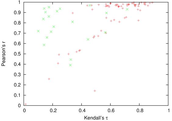
Each point corresponds to a target in benchmark B. The Pearson's r and Kendall's τ are computed from the Pcons MQA. The green points (x) are the 20 assessments with most ties, which inflates the values of Pearson's r.
Figure 2.

Each point corresponds to a target in benchmark B. The Spearman's ρ and Kendall's τ are computed from the Pcons MQA. The green points (x) are the 20 assessments with most ties, which inflates the value of Spearman's ρ.
Figure 3.
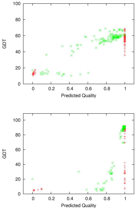
Different MQAs for complete server models of targets T0370 (upper) and T0334 (lower). The set of red points (+) is the MQA from the topranked group (634, Pcons) at CASP7 and the set of green points (X) is our MQA. The correlation values for the assessments in the Figure are: T0370 (+): r=0.94, τ=0.25, ρ=0.60. T0370 (X): r=0.89, τ=0.61, ρ=0.79. T0334 (+): r=0.59, τ=0.14, ρ=0.45. T0334 (X): r=0.54, τ=0.72, ρ=0.90. Evaluations using Pearson's r would slightly prefer the Pcons MQA even though it clearly is not what we expect of a good MQA. However, Kendall's τ and Spearman's ρ are much higher for our assessments, because they do much better rankings of the models.
Other measures, like the ability to select the best model, could also be considered when comparing MQA algorithms, though this approach, relying as it does on a single data points, is very sensitive to noise. In all cases, the individual scatter plots should be examined as the examples in Figure 3 to avoid misleading correlation coefficients.
The naive implementation of Kendall's τ, which simply considers all pairs of points, runs in O(n2). However, the more efficient algorithm by Knight [12] runs in O(n log n), which is not much more expensive than the O(n) algorithms for other correlations. Statistical tools like R [16] include routines for Kendall's τ computations.
3.3 Model Quality Assessment method
Our MQA consists of the following steps which are described in details in the following sections.
Templates and alignments are found using SAM_T06.
The distances between pairs of residues in contact are extracted for each alignment.
For each pair of residues that are in contact in at least one alignment, a consensus distance is computed (the desired distance).
Weighted constraints are constructed from the desired distances.
(Optional) An optimization algorithm selects a subset of constraints using predicted contact distributions.
Each model is scored according to the (selected) distance constraints.
3.4 Templates and Alignments
We use the fully automated SAM_T06 protocol to find templates and compute alignments. SAM_T06 is a profile HMM that excels in detecting remote homologs. The alignments used are local alignments to a three-track HMM [9, 8] using the amino-acid alphabet, the str2 backbone alphabet [10], and the near-backbone-11 burial alphabet [10], with weights 0.8, 0.6, and 0.8 respectively. This is the alignment setting that has worked best in our tests of various alignment methods for maximizing the similarity to a structural alignment—we did not optimize these settings for the MQA application. For each template, there were three such alignments, using the SAM_T2K, SAM_T04, and SAM_T06 multiple-sequence alignments as the base for the local structure predictions and the HMMs.
3.5 Distance Extraction
The next step is to extract the conserved distances of the residue pairs from the alignments. Distance is measured between the Cβ-atoms of the residues (Cα-atoms for glycines). For each alignment, the distances between all Cβ pairs that have a separation of more than 8 residues and a Euclidean distance ≤ 8 Å are stored. We use a chain separation of 8 residues to avoid trivial chain neighbor contacts—we have not yet experimented with different separation cutoffs. We have experimented with various values of the cutoff radius. Small cutoff radii increase the accuracy of the constraints, but fewer constraints are detected. On the other hand, larger cutoff radii generate more constraints, but their quality decreases rapidly because the larger distances are less conserved. Our ad-hoc experiments therefore suggest that a cutoff radius between 7 and 9 Å gives a good trade-off between sensitivity and accuracy.
This distance extraction therefore results in a triangular protein length × protein length table, where a table entry holds the set of all alignment distances between the corresponding pair of residues. Together with each distance, we also store a weight corresponding to the quality of the template from which the distance was extracted. The quality of a template is calculated directly from the E-values of the template. However, we normalize it such that the weight w(E) of an E-value is in the range [0.1:1]
w(E) = 1 therefore corresponds to the highest-quality template (lowest E-value) and w(E) = 0.1 corresponds to the lowest-quality template (highest E-value). The parameter ∊ is an arbitrary very small number for avoiding division by zero.
The Emax value was generally around 36 for the CASP7 targets. Easy targets with many good hits (E <≪ 1) therefore have many hits with weights close to 1. This might be problematic, since this weighting scheme can not distinguish between excellent hits and only fairly good hits, as they are almost equally close to Emin. We have not yet experimented with other weighting schemes, but this problem might be avoided by limiting the number of templates examined, so that targets with several good hits would have much lower Emax values.
3.6 Desired Distances
From the table of distances and weights, a consensus distance for each pair of residues is computed by calculating a weighted average of the observed distances. After this step, the templates and alignments are therefore reduced to a table of so-called desired distances between residues. Each desired distance also has an associated weight (the sum of the weights of the templates where the distances were observed). If two residues have been in contact in many alignments that scored well, the weight is therefore high. Correspondingly, if two residues have only been in contact in few alignments coming from poorly scoring templates, the desired distance will have a low weight. The weights of the desired distances can therefore be interpreted as the confidence of the distance prediction. If two residues have not been observed to be in contact, the desired distance is undefined and the associated weight is 0.
3.7 Weighted Distance Constraints
For each desired distance Dij between residues i and j, we generate a weighted distance constraint. A distance constraint has a minimum distance Aij, desired distance Dij, maximum distance Bij and a weight Wij. For the constraints in our MQA, the minimum and maximum distances are set somewhat arbitrarily to Aij = 0.8Dij and Bij = 1.3Dij. A distance constraint defines a cost function that is a rational function with minimum C(Dij) = −Wij, C′(Dij) = 0, and C(Aij) = C(Bij) = 0:
| (1) |
| (2) |
| (3) |
The α and β parameters define the shape of the function (Equations 4 and 5) and are most easily interpreted in terms of the asymptote at ∞ and the slope at the maximum distance:
| (4) |
| (5) |
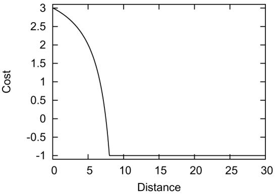
Figure 4 shows a plot of the function with typical settings. The final cost function is the weighted average of the individual costs for all constraints used.
Figure 4.
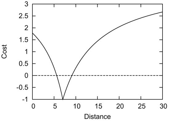
The cost function with parameters Dij = 7, α = 200, β = 50, Wij = 1.
3.8 Selection of Constraints
For the basic MQA method, the model cost function is the sum of all of the cost functions for the pairs of residues, but the method can be improved by using only a good subset of the constraints. We have evaluated several selection strategies and describe two of them here. The selection by fraction strategy is very simple, but improves the performance of the MQA method only marginally. The selection using contact predictions strategy is more complicated, but is the best selection we have tried.
3.8.1 Selection by Fraction
A plot of the error of the constraints vs. their weight is shown in Figure 5 for Target T0370. It clearly shows that high-weight constraints are generally more correct than low-weight constraints. Although we show this property only for one arbitrarily chosen target, a similar relationship holds for most of the targets, though it is strongest for targets for which good templates are available. A simple selection strategy is therefore to sort the constraints by weight and to select a fraction of the highest weight constraints for the final model cost function.
Figure 5.

Each point corresponds to a constraint. The weight of the constraint is shown on the x-axis and the magnitude of the difference between the actual distance in the experimental structure and the desired distance of the constraint is shown on the y-axis. From the scatter diagram, it is easy to see that high-weight constraints tend to have low errors in distance. This property is true for almost all targets considered.
Figure 6 shows the average Kendall's τ for selecting different fractions of the high-weight constraints. The plot shows that the average Kendall's τ for Benchmark A increases from 0.570 using all constraints (100%) to 0.575 when selecting only 40% of the highest weight constraints, but that the quality of our MQA method decreases rapidly when selecting less than 30%. This decline is because we are beginning to discard many good constraints at this point. Even though the increase in average Kendall's τ is small, the result is important because it shows that a proper selection of constraints can improve the performance of our method.
Figure 6.
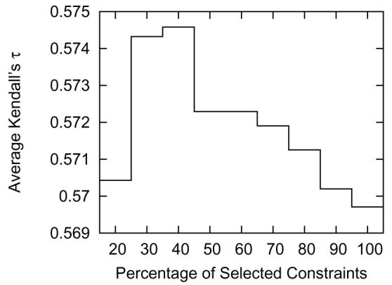
The average Kendall's τ is maximized when selecting approximately 30%–40% of the highest weight constraints.
3.8.2 Selection using Contact Predictions
We can predict how many contacts each residue should have using neural nets, then select constraints so that residues predicted to have more contacts have more constraints also.
We trained neural nets to predict probability Pi,c of residue i having c contacts with separation greater than 8 residues. Residues are said to be in contact if the distance between their Cβ-atoms (Cα-atoms for glycines) is less than 8 Å; the same definition we used for extracting constraints. The contact number predictions are done using the same neural network program (predict-2nd) that we use for all our local structure prediction [11].
Our main selection strategy is to select a subset of constraints that maximizes the contact number probability for each residue, but we also want to have many high-weight constraints. Two objectives must therefore be maximized: the contact number probability and the average weight of the chosen constraints. We used a simple greedy algorithm to do this optimization: Figure 7.
Figure 7.
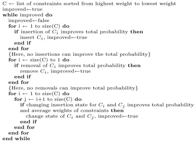
The optimization algorithm for selecting high-weight constraints based on neural-net predictions of the contact number for each residue. Note that each constraint Ci affects the probability for the contact number of two residues. When there are more than 10 000 constraints in set C, we skip the final quadratic-time step, since it offers only small improvements.
The asymptotic running time of the algorithm is O(In2) where I is the number of improvements and n is the number of constraints. In practice the algorithm runs in reasonable time < 5s for problems with fewer than 10 000 constraints. For larger problems, the quadratic-time optimization step is skipped, since it only contributes small improvements compared to the initial linear-time optimization. Using the optimized set of constraints the average Kendall's τ improved from 0.570 using all constraints to 0.582. This selection strategy gives the best improvement in terms of average Kendall's τ of any we have tried, and we do not have to tune a parameter that might be benchmark-dependent like the fraction parameter.
3.8.3 Prediction of non-contacts
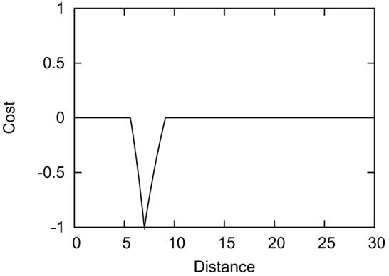
The above selection strategies show how a reduction of the constraint set can improve the quality of the method. We have also found that the addition of so-called non-contact constraints also improves the method substantially. The idea is simply that if a pair of residues is not observed to be in contact in any alignment, then a non-contact constraint is added to the constraint set. This is a special constraint that only penalizes residues being in contact. This behavior can also be modeled with our standard cost function (Equation 1) by setting Dij = 8, Aij = 7.5, Bij = ∞ (in practice, we use 10 000 to be effectively ∞). The non-contact cost function is illustrated in Figure 8.
Figure 8.
The non-contact cost function with parameters Dij = 8, Aij = 7.5, Bij = ∞, α = 200, β = 50.
Using the optimized set of constraints together with the non-contact constraints improves the average Kendall's τ from 0.582 using just the optimized contact constraints to 0.589.
3.8.4 Constraints from Predicted Models
The top-ranked method (Pcons) at CASP7 builds its scoring function from consensus features of the models to be assessed. This approach works very well for CASP MQA since many of the models are of high quality and the consensus features are therefore more likely to be good. Our method for constraint extraction and optimization can easily be generalized to consider the predicted models as well. However, we stress that this approach can only be successful when the model set is large enough to express correct consensus features. In the case of assessing the quality of few models (or one model in the extreme case), the constraints should be extracted from alignments.
When extracting distance constraints from the alignments, we have a clear indication of the alignment quality from the template E-value. This is usually not the case when extracting constraints from predicted models. We therefore performed one experiment where all of the models are equally weighted and another experiment where the models are weighted according to the model cost given by alignment constraints. The results of these experiments are summarized in Table 1. In both experiments there are significant gains when optimizing the constraint sets. However, the qualities of two optimized constraint sets are very similar, which indicates that the optimization algorithm is able to the choose good constraints also in the unweighted experiment.
Table 1.
The all and optimized columns show the average Kendall's tau (Pearson's r in parenthesis) for the two consensus experiments that used constraints extracted from the set of models to be evaluated. All corresponds to selecting all constraints. The optimized column corresponds to the constraints selected by the optimization algorithm described in Figure 7.
| Experiment | All | Optimized |
|---|---|---|
| Equal Model Weights | 0.591 (0.830) | 0.621 (0.863) |
| Weighted Models | 0.598 (0.839) | 0.622 (0.866) |
The performances of the different alignment extraction algorithms and the weighted model extraction algorithm are summarized in Table 2.
Table 2.
Average Kendall's τ and Pearson's r for different versions of the MQA method using Benchmark A. Note that while Kendall's τ is improved by using non-contact constraints, Pearson's r is decreased. The inclusion of non-contacts decreases the linearity of the correlation, but improves the ranking of models. We have argued that we prefer Kendall's τ over Pearson's r, and so we consider the non-contacts to be beneficial to our MQA method.
| Constraint Set | τ̅ | r̅ |
|---|---|---|
| All | 0.570 | 0.825 |
| Best fraction | 0.575 | 0.833 |
| Optimized | 0.582 | 0.838 |
| Opt+noncontacts | 0.589 | 0.827 |
| Opt+models | 0.622 | 0.866 |
4 Results
Here we evaluate our alignment constraints for MQA. This is done by splitting the constraints into three disjoint sets.
alignment constraints These are the constraints that are selected by the optimization algorithm described in Figure 7.
rejected alignment constraints These are the constraints that were not selected by the optimization algorithm in Figure 7.
non-contact constraints Constraints between pairs of residues that were not observed to be in contact in any alignment.
We also consider three additional sets, which are constructed by using a bonus cost functions on the above constraint sets (Figure 9), which provides negative costs, but no positive costs (truncating the standard cost function for a constraint at 0). The total cost function is a weighted sum of costs from the 6 constraint sets. A five-fold cross-validation was done to test the weighted cost function, using the cross-validation and optimization techniques described in the companion paper by Archie and Karplus [3]. We do not report the weights for the various cost functions here, as they came out very slightly different for each train/test split.
Figure 9.
The bonus cost function with parameters Dij = 7, α = 200, β = 50. This type of cost function is 0 when Dij < Aij or Dij > Bij, otherwise it behaves as described in Equation 1. The bonus cost functions are useful for low quality constraints. As the name indicates, a bonus constraint only rewards models when the constraint is satisfied.
We compare our MQA with various MQA methods including the best ranked group at CASP7. This is done using Benchmark B consisting of complete (no missing atoms) server models from CASP7. The results are summarized in Table 3. The table is extracted from the companion paper by Archie and Karplus [3], which describes the statistics and the data used in Table 3. Optimal weights trained on all CASP7 targets are shown in Table 4. Pooled standard deviation is defined by
| (6) |
where 𝕋 is the set of targets, nt is the number of structures for target t, and σt is the standard deviation of the cost function among models of target t. The pooled standard deviation of the weighted cost function component is a useful way of gauging how much the component contributes to the final cost function. It is more informative than the raw weight of the component, because it does not depend on the rather arbitrary scaling of the individual components.
Table 3.
The table shows the average Kendall's τ and average Pearson's r using benchmark B. Correlation is computed separately for each target, then averaged. The Align-all row is the results of MQA with distance constraints from alignments using the 6 constraint sets described here. The Align-only row is the results of MQA with no noncontacts. The Meta-weighted and meta-unweighted rows are the results of extracting constraints from the models to be assessed (with weighted models and unweighted models respectively). TASSER, Lee, and Pcons are top-ranked MQA methods presented at CASP7 (groups 125, 556, and 634 respectively). Qiu is a newer MQA method described in Qiu et al. [15]. The companion paper by Archie and Karplus [3], evaluates our MQA algorithm on more measures.
| Group | τ̅ | r̄ |
|---|---|---|
| Meta-weighted | 0.624 | 0.862 |
| Meta-unweighted | 0.624 | 0.861 |
| Lee | 0.585 | 0.805 |
| Qiu | 0.581 | 0.853 |
| Align-all | 0.574 | 0.832 |
| Align-only | 0.570 | 0.832 |
| Pcons | 0.560 | 0.847 |
| TASSER | 0.538 | 0.633 |
Table 4.
Optimized weights for alignment-based cost functions. Weights were optimized to maximize a weighted measure of correlation (τ3, described elsewhere [3]) with GDT_TS on complete models.
| Cost Function | Weight | Pooled SD |
|---|---|---|
| align_constraint | 9.95242 | 6.16873 |
| noncontacts | 59.6361 | 0.854129 |
| noncontacts_bonus | 30.4114 | 0.300117 |
Figure 10 shows a comparison between our MQA method and the two best MQA methods at CASP7. When comparing our method with Pcons (upper Figure), the plot clearly shows that our algorithm is generally performing better on the easy targets (template-based targets). When comparing our algorithm with the Lee algorithm we, surprisingly, see the opposite behavior: our method does better on the harder targets.
Figure 10.
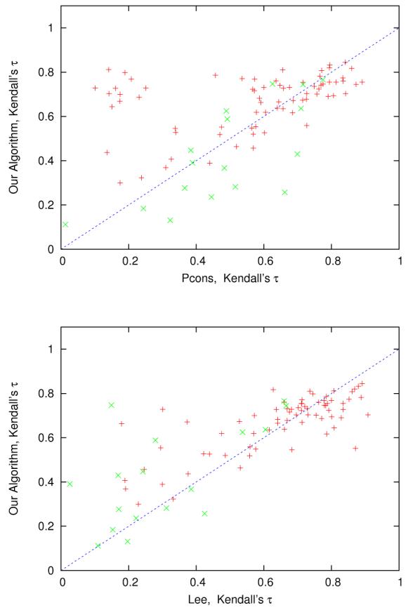
Each point corresponds to a target in benchmark B. Here we show average Kendall's τ using our algorithm (constraints extracted from models) vs. Pcons and the Lee algorithm. Easy targets (marked with red +) correspond to template-based targets and hard targets (marked with green ×) correspond to template-free models using the CASP7 classification.
4.1 Quality of Templates is Important
Since our MQA method is based on homology modeling, the existence of good templates is crucial. It is not possible to know the real quality of a template without knowing the native structure of the target, but the E-value of the template from the search is a good indication of its quality. Figure 11 shows the relationship of the lowest E-value for the target compared to the Kendall's τ for that target. If we find a template with E-value less than 0.9, then the performance of the MQA is generally good, but if the best template E-value is more than 0.9, we can't predict the performance of the MQA based on the E-value only.
Figure 11.
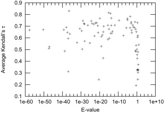
Each point corresponds to a target. The lowest E-value of any template for the target is shown on the x-axis and the Kendall's τ of the models is shown on the y-axis.
The two outliers are T0379 (4E-21,0.244) and T0375 (1.4E-37,0.312). Both targets had many templates and good models from many servers, so that getting a high correlation with quality requires detecting fairly small differences between models. There appear to be two sets of models for both targets (one using a good template and one using a poorer template), with high correlation between the MQA measure and GDT within each set, but without clean separation of the sets.
5 Discussion and Conclusion
We have presented a simple and powerful method for extracting distance constraints from alignments. We have shown how these constraints can be used as a score function for model quality assessment. Our results in Table 3 indicate that MQA using the alignment constraints is comparable in quality to the best methods at CASP7. The distance constraints from alignments are based on evolutionary information only, but are often useful even when sensitive fold-recognition methods do not reliably detect templates.
Even though we here focus on extracting distance constraints from alignments, our algorithm also performs very well when extracting the constraints from the models to be assessed. The models from the CASP7 MQA are generally of high quality and we therefore get a better performance when extracting constraints from the models compared to the alignments. However, in general we can not always expect to have such a large fraction of good models and extracting from alignments seems safer when the method is applied to an unknown collection of models.
When comparing our method with the two best ranked methods at CASP7, we notice that our method is generally better than Pcons on the template-based targets.
On the other hand it is quite surprising that our method performs better than the Lee method on most of the hard targets. The reason for this is that the Lee method only use one predicted base model for comparison. This, of course, works well when the predicted model is good. For the hard targets where our method is doing particularly better than the Lee method, (T0321 and T0350), the base models predicted by the Lee group were poor. Our algorithm therefore seems to be robust on both easy and hard targets.
We have also presented an alternative measure for evaluating an MQA method, the Kendall's τ, and provided several arguments why this measure should be used for future CASP MQA assessments.
6 Acknowledgments
We would like to thank all people who have worked on Undertaker and SAM. Specifically John Archie, who created the test framework and the optimization algorithm for combining cost functions; Grant Thiltgen trained the predict-2nd neural network for prediction of the distribution of contact counts.
Martin Paluszewski is partially supported by a grant from the Danish Research Council (51-00-0336). This research was also supported by NIH grant R01 GM068570.
References
- Altschul S, Gish W, Miller W, Myers E, Lipman D. Basic local alignment search tool. Journal of Molecular Biology. 1990;215:403–410. doi: 10.1016/S0022-2836(05)80360-2. [DOI] [PubMed] [Google Scholar]
- Altschul SF, Madden TL, Schäffer AA, Zhang J, Zhang Z, Miller W, Lipman DJ. Gapped BLAST and PSI-BLAST: a new generation of protein database search programs. Nucleic Acids Research. 1997 September;25(17):3389–3402. doi: 10.1093/nar/25.17.3389. [DOI] [PMC free article] [PubMed] [Google Scholar]
- Archie John, Karplus Kevin. Applying Undertaker cost functions to model quality assessment. Proteins: Structure, Function, and Bioinformatics. 2008 doi: 10.1002/prot.22288. Manuscript in preparation. [DOI] [PMC free article] [PubMed] [Google Scholar]
- Bradley Philip, Malmström Lars, Qian Bin, Schonbrun Jack, Chivian Dylan, Kim David E., Meiler Jens, Misura Kira M.S., Baker David. Free modeling with Rosetta in CASP6. Proteins: Structure, Function, and Bioinformatics. 2005 September;61(S7):128–134. doi: 10.1002/prot.20729. [DOI] [PubMed] [Google Scholar]
- Canutescu AA, Shelenkov AA, Dunbrack RL. A graph-theory algorithm for rapid protein side-chain prediction. Protein Science. 2003 September;12(9):2001–2014. doi: 10.1110/ps.03154503. [DOI] [PMC free article] [PubMed] [Google Scholar]
- Chothia C, Lesk AM. The relation between the divergence of sequence and structure in proteins. EMBO Journal. 1986 April;5(4):823–826. doi: 10.1002/j.1460-2075.1986.tb04288.x. [DOI] [PMC free article] [PubMed] [Google Scholar]
- Cozzetto Domenico, Kryshtafovych Andriy, Ceriani Michele, Tramontano Anna. Assessment of predictions in the model quality assessment category. Proteins: Structure, Function, and Bioinformatics. 2007 August 6;69(S8):175–183. doi: 10.1002/prot.21669. [DOI] [PubMed] [Google Scholar]
- Karchin R, Cline M, Mandel-Gutfreund Y, Karplus K. Hidden Markov models that use predicted local structure for fold recognition: alphabets of backbone geometry. Proteins: Structure, Function, and Genetics. 2003 June;51:504–514. doi: 10.1002/prot.10369. [DOI] [PubMed] [Google Scholar]
- Karplus Kevin, Karchin Rachel, Draper Jenny, Casper Jonathan, Mandel-Gutfreund Yael, Diekhans Mark, Hughey Richard. Combining local-structure, fold-recognition, and newfold methods for protein structure prediction. Proteins: Structure, Function, and Genetics. 2003 October 15;53(S6):491–496. doi: 10.1002/prot.10540. [DOI] [PubMed] [Google Scholar]
- Karplus Kevin, Katzman Sol, Shackelford George, Koeva Martina, Draper Jenny, Barnes Bret, Soriano Marcia, Hughey Richard. SAM-T04: what's new in protein-structure prediction for CASP6. Proteins: Structure, Function, and Bioinformatics. 2005 September;61(S7):135–142. doi: 10.1002/prot.20730. [DOI] [PubMed] [Google Scholar]
- Katzman Sol, Barrett Christian, Thiltgen Grant, Karchin Rachel, Karplus Kevin. Predict-2nd: a tool for generalized local structure prediction. Bioinformatics. 2008 doi: 10.1093/bioinformatics/btn438. Manuscript in preparation. [DOI] [PMC free article] [PubMed] [Google Scholar]
- Knight WR. A computer method for calculating Kendall's tau with ungrouped data. J. Am. Stat. Assoc. 1966;61:436–439. [Google Scholar]
- Mcguffin Liam J. Benchmarking consensus model quality assessment for protein fold recognition. BMC Bioinformatics. 2007 September;8:345+. doi: 10.1186/1471-2105-8-345. [DOI] [PMC free article] [PubMed] [Google Scholar]
- Pearson WR, Lipman DJ. Improved tools for biological sequence comparison. Proceedings of the National Academy of Sciences, USA. 1988 April;85(8):2444–2448. doi: 10.1073/pnas.85.8.2444. [DOI] [PMC free article] [PubMed] [Google Scholar]
- Qiu Jian, Sheffler Will, Baker David, Noble William Stafford. Ranking predicted protein structures with support vector regression. Proteins: Structure, Function, and Bioinformatics. 2008 May 15;71(3):1175–1182. doi: 10.1002/prot.21809. [DOI] [PubMed] [Google Scholar]
- R Development Core Team . R: A Language and Environment for Statistical Computing. R Foundation for Statistical Computing; Vienna, Austria: 2008. ISBN 3-900051-07-0. [Google Scholar]
- Sali A, Blundell TL. Comparative protein modelling by satisfaction of spatial restraints. Journal of Molecular Biology. 1993 December;234(3):779–815. doi: 10.1006/jmbi.1993.1626. [DOI] [PubMed] [Google Scholar]
- Wallner Björn, Elofsson Arne. Prediction of global and local model quality in CASP7 using Pcons and ProQ. Proteins: Structure, Function, and Bioinformatics. 2007 September;69(S8):184–193. doi: 10.1002/prot.21774. [DOI] [PubMed] [Google Scholar]
- Zemla A, Venclovas C, Moult J, Fidelis K. Processing and analysis of CASP3 protein structure predictions. Proteins. 1999;3(Suppl):22–29. doi: 10.1002/(sici)1097-0134(1999)37:3+<22::aid-prot5>3.3.co;2-n. [DOI] [PubMed] [Google Scholar]
- Zhang Yang. Template-based modeling and free modeling by I-TASSER in CASP7. Proteins: Structure, Function, and Bioinformatics. 2007;69(S8):108–117. doi: 10.1002/prot.21702. [DOI] [PubMed] [Google Scholar]
- Zhang Yang, Arakaki Adrian K. K., Skolnick Jeffrey. TASSER: An automated method for the prediction of protein tertiary structures in CASP6. Proteins: Structure, Function, and Bioinformatics. 2005 September;61(S7):91–98. doi: 10.1002/prot.20724. [DOI] [PubMed] [Google Scholar]