Estimating cerebral oxygen metabolism from fMRI with a dynamic multicompartment Windkessel model

Abstract

Stimulus evoked changes in cerebral blood flow, volume, and oxygenation arise from responses to underlying neuronally mediated changes in vascular tone and cerebral oxygen metabolism. There is increasing evidence that the magnitude and temporal characteristics of these evoked hemodynamic changes are additionally influenced by the local properties of the vasculature including the levels of baseline cerebral blood flow, volume, and blood oxygenation. In this work, we utilize a physiologically motivated vascular model to describe the temporal characteristics of evoked hemodynamic responses and their expected relationships to the structural and biomechanical properties of the underlying vasculature. We use this model in a temporal curve‐fitting analysis of the high‐temporal resolution functional MRI data to estimate the underlying cerebral vascular and metabolic responses in the brain. We present evidence for the feasibility of our model‐based analysis to estimate transient changes in the cerebral metabolic rate of oxygen (CMRO₂) in the human motor cortex from combined pulsed arterial spin labeling (ASL) and blood oxygen level dependent (BOLD) MRI. We examine both the numerical characteristics of this model and present experimental evidence to support this model by examining concurrently measured ASL, BOLD, and near‐infrared spectroscopy to validate the calculated changes in underlying CMRO₂. Hum Brain Mapp 2009. © 2008 Wiley‐Liss, Inc.

INTRODUCTION

Functional neuroimaging techniques such as magnetic resonance imaging (MRI) [Belliveau et al., 1991; Ogawa et al., 1990] can record changes in cerebral blood flow, volume, or oxygen saturation that are indirectly related to neuronal activity and reflect the consequences of both neural‐metabolic and neural‐vascular coupling. Although the ability to image these signals has been invaluable in developing spatial maps of the functional organization of the brain, the dependence of measured hemodynamic signals on both vascular and metabolic function results in ambiguous and potentially nonlinear relationships with the underlying electrophysiological and metabolic responses. The potential use of cerebral oxygen metabolism (CMRO₂) as a more accurate indicator of neuronal activation has motivated the recent development of model‐based methods to extract these estimates from functional MRI (fMRI) or optical measurements (reviewed by [Buxton et al., 2004]).

The majority of studies that have been performed to estimate CMRO₂ by fMRI methods have focused on examining the magnitude of evoked signals. In many cases, these studies have used long duration functional stimulation and steady‐state approximations of the vascular and oxygen transport models. In addition, many of these studies rely on a hypercapnic calibration of the blood oxygen level dependent (BOLD) signal, as introduced by Davis et al. [1998], to calibrate the magnitude of signal changes; as these depend on the baseline physiological and biophysical properties of the vasculature. However, such studies have largely overlooked the potential to utilize the temporal dynamics of the hemodynamic measurements and the inter‐relationships between the flow, volume, and oxygen‐saturation changes, which can reveal information about the underlying biomechanical properties of the vasculature, such as vascular transit time, vascular compliance, and baseline vascular features. Several recent experimental studies have demonstrated that baseline blood flow, volume, and venous oxygen saturation can have significant effects on the relative temporal characteristics of the overall hemodynamic changes (e.g., [Cohen et al., 2002; Liu et al., 2004; Sicard and Duong, 2005]). In light of such experimental data, we hypothesized that the utilization of dynamic information from multimodal measurements will help to characterize flow and oxygen metabolism changes more accurately by providing additional information about the properties of the vascular network based on the relationships of both the temporal evolution and magnitude of the evoked hemodynamic signals.

Several recent studies have described bottom‐up methodologies that use model‐based curve‐fitting of the hemodynamic response to estimate the underlying vascular and metabolic states [Deneux and Faugeras, 2006; Huppert et al., 2007; Riera et al., 2005]. In this work, we extend our previous model described in Huppert et al. [2007] to use high‐temporal resolution, multimodal measurements to estimate parameters depicting the vascular biomechanics. We find that this approach allows us to estimate dynamic changes in CMRO₂ from measurements of blood flow and BOLD evoked changes by using our vascular model as the basis for a nonlinear inverse problem. We present three examples to demonstrate the advantages and limitations of the inverse problem by examining (i) the local sensitivity and stability of the inverse problem, (ii) the global robustness of the parameter identification procedure, and (iii) the application of our model to experimental data. In the experimental data, we estimate relative CMRO₂ changes from blood flow and BOLD responses measured during the performance of a brief motor task activity as measured by pulsed arterial spin labeling (ASL) imaging. Finally, we compare the results of this analysis of fMRI signals with the analysis of measured changes in blood flow, volume, and oxygen saturation obtained using simultaneously measured fMRI and near‐infrared spectroscopy (NIRS) data.

METHODS

Overview of Model

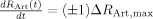
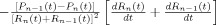
In our dynamic model, evoked changes in the vascular tone and the cerebral metabolic rate of oxygen (CMRO₂) are estimated by the inversion of a nonlinear model that describes the changes in blood flow, volume, and oxygenation in response to the driving forces as schematically depicted in Figure 1A. Our approach is similar to that discussed in previous works [Deneux and Faugeras, 2006; Huppert et al., 2007; Riera et al., 2005]. Our model can be divided into three components: (i) a dynamic forward model that describes the physiological response of the vascular system to flow and CMRO₂ changes (sections “vascular forward model” and “oxygen transport forward model”); (ii) the observation model that describes the biophysics of the fMRI or optical measurement process (section “hemodynamic observation models”); and (iii) the inverse model that estimates values of the input states and parameters via a measurement variance weighted least‐squares fit of experimental data (section “the vascular inverse model”). The details of this forward model have been presented previously. [Huppert, 2007; Huppert et al., 2007].

Figure 1.

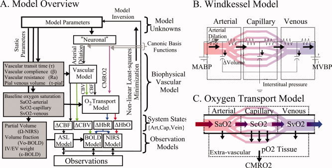
Schematic outline of the vascular model. A vascular forward model (Panel A) based on a multicompartment Windkessel (Panel B) and oxygen transport model (Panel C) is used to estimate the changes in blood flow, volume, and oxygenation in the arterial, capillary, and venous compartments. The model of hemodynamic signals is evoked by underlying changes in vascular tone via arterial vasodilatation and changes in the cerebral metabolic rate of oxygen (CMRO₂). Observation models depicting the biophysics of the optical and fMRI techniques relate the internal states of the model to the measurable hemodynamic responses, which are compared with experimental data.

Vascular forward model

The vascular component of this model is derived from basic principles of fluid mechanics and is based on the flow and volume changes within a system consisting of a dilating arteriole, two compliant vascular windkessel compartments and a constant volume compartment that models the pial veins as depicted in Figure 1B and is summarized in Table I. Briefly, the blood flow between each vascular compartment (F _n−1,n) is derived from the gradient of the hydrostatic pressure (P_n) between the compartments and the vascular resistance of the blood vessels (R_n). The vascular resistance is inversely related to the diameter of the blood vessels according to Poiseuille's law [Washburn, 1921] and thereby related to vascular volumes. A decrease in arterial resistance drives an increase in blood flow. The resulting hydrostatic pressure between the vascular compartment and the surrounding tissue (P _surround) causes an increase in the vascular blood volume (V_n). As the capillary and venous vascular compartments expand against the surrounding tissue, the extra‐vascular space resists compression that gives rise to a saturation of the volume expansion function. Thus, the vascular capacitance (C_n) decreases as a function of the pressure gradient between the compartment and the surrounding tissue [Mandeville et al., 1999b]. In the aforementioned variables, n indicates the vascular compartment (arterial, capillary, vein or pial vein).

Table I.

Summary of Windkessel model

Arterial dilation contraction (arterial resistance state)

Flow changes

Volume changes

Pressure changes

Resistance changes

Capacitance changes

The temporal dynamics of cerebral vascular changes can be approximated based on the fluid mechanics of a compliant Windkessel compartment. In response to changes in vascular tone (described as a sum of two independent non‐linear gamma‐variant temporal basis functions), the flow, volume, and pressure changes are modeled for each of the three vascular compartments (n ∈ {Artery, Cappilary, Vein}). The symbols used in the equation above are P, pressure; F, blood flow; V, blood volume; C, capacitance; R, vascular resistance; and t, time. The subscript ‘0’ indicates the baseline value. In the arterial resistance equation, H(t) is the heavy side hat function. Further details of this model have been presented in (Huppert et al., 2007).

In our model, we assume that the changes in vascular resistance can be approximated using a canonical driving function to the vascular system similar to the canonical neurovascular model described in Buxton et al. We define the dilation and contraction of the arteries as the sum of a pair of independent canonical γ‐variant temporal basis functions with variable timing parameters (refer Table I: Arterial Dilation). We use these nonlinear canonical functions with variable onset time (τ_onset), width (σ), and amplitude, to impose a smooth temporal basis for the arterial resistance state instead of modeling the entire time‐series of arterial dilation. A total of six unknown model parameters describe the arterial dilation and contraction states (refer Tables I and III].

Table III.

Description of parameters in Model

	Symbol	Description	Physiological range	Citation
Arterial resistance temporal basis	ΔRAlmax	Maximum change arterial resistance	[0–90] [−90–0]%	—
	τonset	Time to onset of resistance change	[0–6]s [0–6]as	—
	σA	Width of temporal resistance change	[0–8]s [0–8]s	—
CMRO2 temporal basis	ΔCMRO2Max	Maximum change in relative CMRO2	[0–50]%	—
	τonset	Time to onset of CMRO2 change	[0–4]s	—
	σM	Width of temporal CMRO2 change	[0–8]s	—
Vascular model parameters	RA(0)	Initial arterial resistance	[20–90]%	(Boas et al., 2003)
	β	Windkessel vascular reserve	[1.1–5]	(Mandeville et al., 1998b)
	τ	Vascular transit time	[0.5–4]s	(Ito et al., 2005)
	τpial	Pial venous transit time	[0–4]s	—
Oxygen saturation	SaO2	Baseline arterial saturation	[95–100]%
	ScO2	Baseline capillary saturation	[60–90]%b	(Herman et al., 2006)
	SvO2	Baseline venous saturation	[55–89]%b
NIRS lead field	[HbT]0	Total baseline blood volume	[40–140]μM	(Tomcelli et al., 2001)
	ωpial	Pial vascular sensitivity	[0–1]	—
BOLD lead field	Vo	Baseline vascular volume fraction	[1–10]%	(Ito et al., 2005)
	ε	Intrinsic ratio of intra/extra‐vascular signal	[1–5]	—

This table shows the parameters used in the model described in the text. Physiological ranges are used to set the upper and lower bounds for each parameter used in the fitting procedure as determined from the provided citations. The baseline oxygen saturation of each vascular compartment was estimated in the full multimodal model only.

^aOnset time for the arterial contraction response is defined as the lag time after the onset of the dilation response.

^bCapillary and venous oxygen saturations are defined by the change from the previous compartment to ensure that S_aO₂ > S_cO₂ > S_vO₂.

Oxygen transport forward model

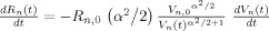
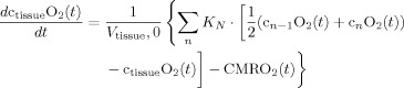
In the second part of the physiological forward model, net changes in blood oxygenation are modeled by a set of first‐order differential equations that describe the balance between the oxygen supplied by the vascular response and the oxygen consumed within the tissue. We calculate the oxygen content (c_nO₂; designating the nth compartment) in both the vascular segments and the bulk extra‐vascular parenchyma tissue using the oxygen transport model described in previous works [Herman et al., 2006; Huppert et al., 2007]. The rate of transport across each vascular segment can be described by first‐order rate equations and depends on (i) the steady‐state flow and (ii) the relative permeability of the segment, which can be determined from the baseline oxygen saturation.

Increased CMRO₂ in the extra‐vascular compartment is approximated by a canonical temporal basis function as described in previous works [Huppert et al., 2007]. As with the arterial resistance state, CMRO₂ changes are described by a γ‐variant functional form (refer Table II). Both the timing and amplitude of this function are estimated as parameters within the model. Unlike arterial resistance changes only one basis function is used as a regressor maintaining that evoked CMRO₂ changes are expected to be elevated compared with baseline.

Table II.

Summary of Oxygen transport model

CMRO2 state

Intravascular oxygen content

Hemoglobin oxygen saturation

Oxy/deoxyhemoglobin changes

Extravascular oxygen changes

Changes in blood and tissue oxygen content are defined a set of differential equations shown in this table derived from the mass‐balance of oxygen delivered via blood flow and consumed via CMRO₂ in the tissue (Huppert et al., 2007). The symbols used in the equations above are as follows: F, flow; V, volume; c_nO₂, oxygen content; s_nO₂, blood oxygen saturation fraction; K_n, vascular permeability rate constant; HbR/HbO₂, deoxy/oxyhemoglobin per volume tissue; H_n, Hufner number (1.39 ml/gm Hb (Habler and Messmer 1997)); HGB‐ hemoglobim content of blood (∼12–15gm Hb/dl (Habler and Messmer, 1997)), and t, time. The subscript ‘0’ indicates the baseline value. In the CMRO₂ equation, H(t) is the heavy side hat function.

Hemodynamic observation models

The second component of our overall model is a set of observation equations that represent the relationships between the underlying physiological variables in the model and the fMRI or optical measurements. Such an unified model of the physiology allows different multimodal information to be fused into a single consistent estimate of cerebral activation. This provides a mechanism to combine both complementary measurements such as BOLD and flow, with partially redundant information, such as the common deoxy‐hemoglobin contrast between optical and BOLD signals. Because these measurement models are modular, this framework allows combinations of the different data sets, namely fMRI, optical, or multimodal data sets, to be utilized and examined for consistency.

FMRI measurement model

The BOLD signal has a complex origin arising from both intra‐ and extra‐vascular water signals [Buxton et al., 2004; Nair, 2005; Obata et al., 2004; Ogawa et al., 1990]. In our model, we consider the contributions to the BOLD signal of all four vascular compartments (artery through pial veins) and susceptibility effects on the extra‐vascular water signal. We model the BOLD signal according to the equations for intra‐ and extra‐vascular contrast described in Obata et al. [2004] based on the theory by Yablonskiy and Haacke [1994].

(1)

Extra‐vascular signal:

Intra‐vascular signal (nth compartment):

At the 3 T field strength used in this study, r _o = 100 s⁻¹ and v _o = 80.6 s⁻¹ [Mildner et al., 2001]. S _IV and S _EV are the fractional baseline contributions of the intra‐ and extra‐vascular signals, respectively. These parameters include a bulk representation of the intrinsic relaxation rates of water molecules in the intra‐ and extra‐vascular space. Because there is debate over the exact value of this parameter [Lu and van Zijl, 2005; Mildner et al., 2001], we include it as an additional unknown parameter () estimated by the model. In the above equations, V_n is the ratio of blood volume of the nth compartment to tissue volume. The term, V ₀, represents the baseline volume fraction and acts as a partial volume correction factor for the BOLD measurement (i.e., 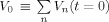). V ₀ is estimated in the model using the minimization procedure and is included as a calibration factor for the magnitude of the BOLD signal. Because this factor has explicit physiological meaning, its value contributes to the calculation of the baseline physiological values.

The measurement sensitivity weighting factors (w_n) in Eq. (1) are assumed to be equal for all four vascular compartments (w_n = 1). The measurement sensitivity factors describe the intrinsic sensitivity of the measurement process and depend on MR physics, the physical vessel dimensions, and vessel orientations. In general, the MR measurement sensitivity is a highly complex function of the underlying vasculature (e.g., [Boxerman et al., 1995]). Our current assumption of equal measurement sensitivities implies that the vascular contributions to the signal directly reflect the relative changes in contrast. For example, the largest contribution to the BOLD signal arises from the venous compartments because the oxygenation changes are the largest in these veins due to washout effects. This assumption should be examined more closely in future work. We use a direct projection of the normalized arterial blood flow changes to model the ASL signal.

NIRS measurement model

The NIRS technique measures spectroscopic changes in the optical absorption properties of tissue [Obrig et al., 1996; Villringer and Chance, 1997]. These measurements are related to changes in mean oxy‐ and deoxy‐hemoglobin concentrations by the modified Beer‐Lambert law [Cope et al., 1988; Delpy et al., 1988]. We assume that the measurements reflect the weighted sum over the vascular compartments, i.e.,

(2)

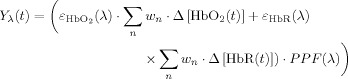
In this equation, ε(λ) is the molar extinction coefficient of each hemoglobin species and PPF(λ) is the effective path‐length for wavelength (λ) traveled by photons on the diffuse path through the brain cortex [Hiraoka et al., 1993]. The subscript n indicates the vascular compartment. In principle, NIRS measurements are related to the absolute changes in hemoglobin concentrations provided that the effective path‐lengths are known [Cooper et al., 1996]. However, in practice, such path‐length factors are difficult to determine without additional spatial information [Hiraoka et al., 1993; Huppert et al., 2006a] or direct measurement [Duncan et al., 1995; Leung et al., 2006]. In our model, hemoglobin changes are normalized to the baseline volume and therefore the value of absolute baseline total hemoglobin is needed to scale between the changes predicted in the model and the true measurements. We include a scaling value (Ω_NIRS) as an additional parameter in the model to compensate for the uncertainty introduced in the exact quantification of the hemoglobin changes measured with NIRS. The measurement model for NIRS is given by the equation

(3)

Note that if the optical path‐length is known then the scaling factor can be used to calculate the baseline hemoglobin concentration (). The normalized term can be calculated directly from within the model. The vascular weights (w_n) in Eqs. (2) and (3) describe the sensitivity of NIRS to the vascular compartments and are assumed to be uniform for the arteries through veins (w_n = 1). The pial venous compartment constitutes larger blood vessels and contributes to changes measured by both the fMRI and optical imaging. Sensitivity to vessels decreases with increasing radius for NIRS measurements [Liu et al., 1995] and conversely increases for gradient echo BOLD‐fMRI [Boxerman et al., 1995]. Therefore, to account for measurement discrepancies, the weight given to the contribution of the pial vein in the NIRS measurement is included as an additional model parameter (ω_pial < 1). This allows the NIRS and BOLD measurements to potentially have different weights for the pial compartment and these measurements can be modeled to sample different effective pial compartments.

The vascular inverse model

There are a total of 20 unknown parameters in the full model (see Table III). The full data model utilizes measurements of blood flow, volume, and oxygen saturation from combined multimodal optical and ASL data. The baseline oxygen saturation contents of the arterial, capillary, and venous compartments have been included as three parameters within the model. These oxygen saturation parameters were fixed in the models using the fMRI only and optical only data. In the fMRI alone and NIRS alone models, there are a total of 15 unknown model parameters because we fix the values for baseline oxygen extraction parameters and additionally drop two parameters specific to NIRS/fMRI, respectively.

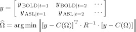
CMRO₂ and arterial resistance changes together with the unknown parameters associated with the model's differential equations can be determined from the inverse of the model. These parameters are estimated by nonlinear curve fitting of the temporal dynamics of observable hemodynamic parameters. We used a nonlinear Levenberg‐Marquardt algorithm [Marquardt, 1963] implemented in Matlab (The Mathworks, Natick, MA) to calculate the model parameters that define the CMRO₂ and arterial dilation functions (Matlab function lsqnonlin). In contrast to previous approaches that consider only the magnitude of hemodynamic changes, we account for the full temporal dynamics of the response and minimize the model using the entire time course of the hemodynamic changes in a single cost function. Thus, the model is minimized using the temporally vectorized array of discrete measurements to simultaneously fit the entire dataset, i.e.,

(4)

where R is an estimate of the variance of the measurement error for each measurement type and superscript T indicates the transpose operation. The estimates of the measurement error variances were calculated from the error in the estimate of the mean evoked hemodynamic responses calculated from the linear deconvolution model (described in section “preprocessing of evoked hemodynamic responses”) from each experimental session and normalized across the subjects. Weighting the squared model error of the different measurement types in the minimization cost function helps to weight the model fit to more confident observations. This routine provides the minimum variance unbiased estimator for a general linear model as described in Huppert et al. [2007] and allows the fusion of multimodal information using a priori knowledge of the measurement error in each imaging method. In the model‐fitting routine, the error cost metric is minimized by refining the model parameters. To improve the stability of the inverse problem, we constrain the parameter set within the range of physiological bounds (Table III). The fitting routine was iterated until a predefined convergence criterion (10⁻⁶ times the variance of the measurement error) was met. This took ∼6–10 h per fitting procedure (Pentium(R)‐4 CPU 3.00 GHz). The error bounds of our model prediction were examined using a Markov Chain Monte Carlo sampling of the parameter‐space as described in Huppert et al. [2007]. Because of the high computational time involved, it is currently impractical to run this model on a per voxel basis, but will be explored in future extensions of this work.

Estimation of baseline physiology from model parameters

In our previous work [Huppert et al., 2007], we described how values for the baseline physiology could be extracted from the model estimates of baseline volume, vascular transit time, and baseline oxygen saturation. For example, the vascular mean transit time, which is defined as the ratio of baseline blood volume and flow, can be estimated from the temporal delay between the arterial (i.e., ASL flow) and venous (i.e., BOLD) responses. These biomechanical parameters provide a link between the dynamics of the evoked response and the baseline state. In addition, both baseline hemoglobin concentration ([HbT₀]) and baseline vascular volume fraction (V ₀) are estimated in the model as the scaling factors applied to the NIRS and BOLD observations, respectively, (detailed in [Huppert et al., 2007]). These calibration factors allow us to assign a physiological scale to the normalized changes estimated in the model.

The estimates of baseline blood volume fraction from the BOLD measurement model (or equivalently total hemoglobin concentration) and the mean vascular transit time (τ) are sufficient to estimate the value of baseline blood flow using the steady‐state relationship,

(5)

where MW_Hb is the gram molecular weight of hemoglobin (64.5 kDa) and ρ_tissue is the density of brain tissue (= 1.04 g/ml [DiResta et al., 1991]). When the full set of measurements (ASL, BOLD, and NIRS) is used to cross‐calibrate the estimates of absolute values for the baseline blood volumes, the ratios of the vascular volume fraction (in volume blood per volume tissue), and baseline hemoglobin concentration (moles Hb per volume tissue) can be used to calculate the hemoglobin content of blood (HGB) in g Hb/volume blood. In the absence of estimates of both V ₀ and [HbT₀], in Eq. (5) HGB can be assumed from literature or measured (in adult humans HGB is typically 12–18 g/dL [Habler and Messmer, 1997]).

At baseline steady state, relative CMRO₂ is the product of blood flow and the oxygen extraction fraction across the compartments. In this model, baseline oxygen saturation is either estimated (using the full multimodality data set only) or assumed from the analysis of the complete data set. Thus, baseline CMRO₂ is calculated directly from the baseline blood flow and absolute oxygen extraction (OE; OE = s_inO₂ − s_outO₂),

(6)

where H_n is the Hufner number (H_n = 1.39 ml O₂/g Hb [Habler and Messmer, 1997]).

Experimental Methods

The data used in this study previously published in [Huppert et al., 2006b] and recorded simultaneous pulsed arteriole spin labeling (PASL) and NIRS measurements. Five subjects were included in this study (4 male and 1 female). Subjects performed a brief 2‐s duration finger walking task using their right hand. All subjects were right‐handed. The stimulus was jittered evenly on a 500‐ms time‐step, which allowed for the response to be estimated at 2 Hz with fMRI. The length of the inter‐stimulus interval (ISI) ranged between 4 and 20 s with an average ISI period of 12 s. The timing of the stimulus presentation was synchronized with the MR image acquisitions and generated with a custom written Matlab script. Each run lasted 6 min and consisted of between 27 and 32 stimulus periods. This was repeated 4–6 times for each subject during the course of one scan session (∼90 min in total time for each session including position of the NIRS probe and structural scans). The human research committee at the Massachusetts General Hospital approved all protocols.

NIRS acquisition

The NIRS probe consisted of two rows of four detector fibers and one row of four source fibers arranged in a rectangular grid pattern and spaced 2.9 cm between nearest neighbor source‐detector pairs as shown in Figure 2. The probe was secured to the subject's head over the contra‐lateral primary motor cortex (M1). This was verified using vitamin‐E fiducial markers in the anatomical MRI. NIRS measurements were taken using a multichannel continuous‐wave optical imager (690 and 830 nm; 18 and 7 mW, respectively) (CW4 system, TechEn Inc., Milford, MA). These signals were synchronized to the timing of the fMRI. Monte Carlo simulations were used to determine the mean photon trajectories by simulating the diffusion through tissue‐segmented anatomical volumes for each subject using the locations of the optodes referenced by the fiducial markers [Huppert et al., 2006a]. A mean partial path‐length correction of 4.7 ± 1.5 and 4.8 ± 1.5 (830 and 690 nm, respectively; N = 5) was calculated from the fraction of the path‐length through the brain cortex based on these simulation results (see Fig. 2B). Methods and results for the collection of this data set have been previously published in Huppert et al. [2006b]. Optical data was sampled at 100 Hz and down‐sampled with a Nyquist filter to 10 Hz for analysis in the model.

Figure 2.

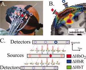
Optical imaging setup. In this figure, we illustrate the setup used for NIRS recordings. Further details can be found in [Huppert et al., 2006b]. Panel (A) shows the location of the optical probe over the motor cortex for a example subject. The “+” indicate the locations of the light source fibers and “o” indicate the detector fiber positions. In Panel (B) is shown a coronal cross‐section of the subjects anatomical MRI with the fiber positions and measurement sensitivity profiles (contour plot) overlain as described in Huppert et al. [2006a]. The BOLD response (thresh held at P < 0.05) is also overlain on the anatomical image. The dotted line in Panel A shows the approximate location of this slice. In Panel (C) is shown the averaged evoked hemoglobin responses from the performance of the motor task. The locations of the axis indicate the originating pair of source and detector positions for the plotted response.

Functional MRI acquisition

Pulsed ASL measurements were carried out at 3 T on a Siemens Allegra MR scanner using PICORE (proximal inversion with control for off‐resonance effects) labeling geometry [Wong et al., 1997] with Q2TIPS (second version of quantitative imaging of perfusion by using a single subtraction with addition of thin‐section periodic saturation after inversion and a time delay sequence) saturation [Luh et al., 1999] to impose a controlled label duration. A post‐label delay of 1400 ms and label duration of 700 ms were used, with repetition and echo times of 2 s and 20 ms, respectively [α = 90°]. Echo Planar Imaging (EPI) was used to image five 6‐mm slices (1 mm spacing) with 3.75 mm in‐plane spatial resolution. The PICORE labeling scheme allowed collection of BOLD signals using the interspersed control images from the acquisition. The fMRI images were motion‐corrected [Cox and Jesmanowicz, 1999] and spatially smoothed with a 6 mm Gaussian kernel. Blood flow and BOLD signals were separated by first extracting the even‐numbered (ASL label and BOLD contrast) and odd‐numbered (BOLD contrast only) series of images. These two time‐series were independently interpolated using cubic spline functions and then the temporally aligned series were subtracted to yield the isolated spin‐label contrast. This approach was similar to the linear “surround subtraction” method described by Lu et al. to give the minimal cross‐talk between the ASL and BOLD signals [Lu et al., 2006]. Structural scans were performed using a T1‐weighted MPRAGE (magnetization prepared rapid gradient echo) sequence [1 × 1 × 1.33 mm resolution, TR/TI/TE/α = 2530 ms/1100 ms/3.25 ms/7°].

Preprocessing of evoked hemodynamic responses

Both the NIRS and fMRI hemodynamic responses were separately estimated using a 2‐Hz resolution finite impulse response (FIR) linear model as described in Huppert et al. [2006b]. High temporal resolution was achieved by designing the stimulation protocol using a jittered inter‐stimulus interval and lowering spatial coverage and resolution for the EPI sequence. This may limit the use of this method in general studies but were necessary to get the effective sample rates needed for our model analysis. The FIR approach assumes a linearly additive hemodynamic model to estimate the high‐temporal resolution responses but avoids canonical assumptions that could restrict the temporal characteristics of the estimates. Second order linear trends were removed from the estimated responses. The epoch timing for this deconvolution was based on the stimulus presentation timing rather then the subject's motor response. However, the subject motor response times were similar to presentation times with a jitter of ∼100 ms as judged by an optical sensor placed on the fingers which was used to record the tapping event as described in Huppert et al. [2006b]. Because of technical limitations, this recording was only available on three of the five subjects. Region‐of‐interest averages for both data sets were independently chosen from measurements showing statistical changes (P < 0.05) based on mixed effects analysis using an activation time window of 2–7 s to define the t‐statistic as described in Huppert et al. [2006b]. The fMRI responses were restricted to voxels beneath the optical probe judged manually based on the fiducial markers on the probe. ASL and BOLD responses were independently estimated. Significant NIRS channels were defined based on the oxy‐hemoglobin estimate.

The resulting BOLD, ASL, and NIRS time‐courses for each subject were variance normalized and averaged into a single group average. In this work, the high computational load of the inverse routine required us to predetermine the single‐trial hemodynamic response function using the FIR model rather than run our state‐space analysis directly on the full data set (c.f. [Deneux and Faugeras, 2006]). However, the linear assumption of the FIR model can be justified (e.g., [Cannestra et al., 1998]) for the minimum inter‐stimulus interval (>4 s) used in this study. We acknowledge that the temporal resolution is limited by the acquisition techniques of fMRI and ASL methods and may currently limit the utility of this method in general studies because the response characterization of our vascular model makes use of high‐temporal resolution response to estimate the vascular parameters.

RESULTS

The underlying vascular and metabolic changes are provided by a nonlinear inverse solution to our vascular forward model and estimated by curve‐fitting the observed hemodynamic responses. To illustrate the performance of this inverse model, we demonstrate the characteristics of our model using three examples that examine the local precision, global accuracy, and physiological consistency of our model when used to analyze fMRI, NIRS, or multimodal data.

Example 1: Parameter Sensitivity and Local Stability of the Inverse Problem

A requirement of a well‐poised inverse model is that the number of independent measurements is equal to or greater than the number of free model parameters. This is informally referred to as the “counting rule” and can provide a qualitative common‐sense check for such a model (e.g., [Bamber and van Santen, 2000]). To begin our investigation of our windkessel model, we will first discuss this qualitative rule. Our model used for analysis of the fMRI signals has a total of 15 free parameters. Although the ASL and BOLD responses (recovered at 2 Hz) contain a greater number of sample points, each sample point does not represent an independent measurement due to the inherent temporal autocorrelation of the evoked response and partial correlation between measurements. To apply the counting rule, we must estimate the number of independent degrees‐of‐freedom to these measurements. The BOLD response is believed to have up to three distinct phases; an initial dip period, a main response, and a post‐stimulus undershoot. To correctly model the overall BOLD response, for example in a general linear model, three independent canonical functions should be used with one for each of these phases. Because each canonical function requires three degrees‐of‐freedom for the amplitude, first order timing (e.g., onset or time‐to‐peak) and second order timing (e.g., temporal width), it follows that a total of nine parameters should be included to model all three phases of the BOLD response. Similar arguments can be applied to determine that oxy‐ and deoxy‐hemoglobin are expected to contain nine degrees‐of‐freedom each and flow to contain six (with an assumption of no “initial dip” period). By this argument, we can expect that the BOLD/ASL fMRI data should have the minimum number of independent degrees‐of‐freedom needed for our model. This argument, however, is at best only a qualitative deduction. To more rigorously investigate the ability to determine all model parameters from fMRI measurements, we must turn to more formal mathematical definitions of model sensitivity and parameter identifiability.

The stability of our inverse model indicates the feasibility of our model to estimate the model parameters from experimental data and requires that measurements be sensitive to changes in each of the estimated model parameters (reviewed in [Bamber and van Santen, 2000]). Model sensitivity can be examined using a variety of numerical methods and has been recently discussed in the context of a similar vascular model by [Deneux and Faugeras, 2006]. However, model sensitivity does not guarantee that the estimated values are accurate or unique. Instead, it allows us to test whether a solution to the inverse problem exists. Because of the nonlinear nature of our model, we focused on local data perturbation methods to examine the theoretical sensitivity of measurements to changes in the model parameters.

Model sensitivity quantifies the influence of each parameter on the output of the forward model. Two parameters; namely, the mean vascular transit time (τ) and the Windkessel vascular compliance factor (β), are primarily involved in modeling the dynamic relationship between flow and volume. We begin our investigation of model sensitivity by qualitatively examining whether these two parameters affect the temporal dynamics of the hemodynamic response and if it is plausible to estimate these values based on relative temporal dynamics. On the basis of our model, we predicted that these two parameters would have distinguishable effects on the relative temporal dynamics of the BOLD and ASL measurements. For example, in Figure 3A we see that if vascular transit time is increased (i.e., with constant baseline flow and thus increased baseline volume), the BOLD response amplitude is reduced and the initial dip component is removed. In particular, a longer transit time increases the temporal delay between arterial and venous responses. Likewise, increases in the value of β lead to larger and quicker washout changes that produce larger magnitude changes in BOLD and deoxy‐hemoglobin and reduce the relative time‐to‐peak value of these responses. The compliance parameter also has pronounced effects on the relative magnitude (i.e., ratio) of the oxy‐, deoxy‐, and total‐hemoglobin changes that are measured by NIRS reflecting differing degrees of washout. We note that the relationships between multimodal measurements are uniquely related to these parameters when compared with the individual evoked responses considered independently.

Figure 3.

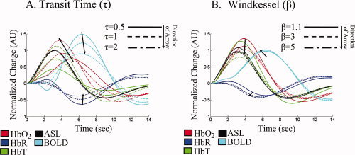
Parameter sensitivity of the evoked hemodynamic response. This figure illustrates the effect of the biomechanical properties of the vascular network on the temporal dynamics of evoked response. Panels (A) and (B) show qualitatively how the simulated evoked responses vary with different values for the mean vascular transit time (τ) and Windkessel parameter (β). The magnitudes of the responses are normalized to the peak response for each measurement type in order to facilitate cross‐modality comparisons.

The sensitivity of our model each parameter in the model can be numerically quantified by examining the Jacobian of the model with respect to the model parameters. We examined the rank and condition of the Jacobian throughout the bounds of the parameter space to determine if the set of measurements was sensitive to each model parameter. We examined these properties for the full multimodal, BOLD and ASL, and NIRS observation models. We found that the Jacobian was full rank for the parameters estimated in each of these models, which implies that an inverse of the model around a localized point is theoretically possible. Singular value decomposition of the Jacobian provided similar conclusions and showed that the number of independent components was equal to the number of model unknowns (for further discussion refer to [Huppert, 2007]). In comparison, when we examined the model with BOLD only measurements, we found that it was not possible to uniquely estimate many of the parameters of the model, including the separation of flow and consumption changes (i.e., the Jacobian was no longer full rank). This finding was consistent with the previous results from Deneux and Faugeras [Deneux and Faugeras, 2006], which attempted similar analysis of BOLD signals alone and found that many but not all of their model parameters could be independently determined. Here, we find that if we use both ASL and BOLD measurements, the model is better defined because information about the model parameters can be additionally determined from the inter‐relationships of these signals. To further explore the limits of the model, we examined the Jacobian of each model as a function of the simulated sample frequency and determined that the minimum acquisition speed needed was approximately half of the mean transit time. This implies that the estimation of this model will require a minimum sampling rate of above 1 Hz for both flow and BOLD signals, which is unfortunately faster than is possible in most current fMRI studies and was only possible in this study using jittered stimulation presentation.

A further metric of model sensitivity is the variance inflation factor (Γ), which quantifies the minimum uncertainty that can be theoretically expected in the estimate of each model parameter based on an analysis of the slope (Jacobian) of the minimization function around a given local model solution. This analysis allows us to examine how distinguishable the effects of one parameter are from the other parameters. Using the notation discussed in [Deneux and Faugeras, 2006], for a small change in one parameter (θ_i), the perturbation of the observation varies by J_idθ_i, where J_i denotes the Jacobian of the forward model with respect to the ith parameter. If the Jacobian associated with the parameter under consideration is not orthogonal to the Jacobian matrix with respect to the remaining parameters (denoted J _φ), then the cross talk between parameters results in nonuniqueness of the solution because an error in one parameter can be compensated by errors in other parameters. The maximum precision of each parameter can be estimated for a given level of noise in the measurements from the variance inflation factors as described in Deneux and Faugeras [2006] using the following equation.

(7)

where represents the transpose of the Jacobian matrix. The smaller the corresponding diagonal element of the variance inflation matrix (Γ_i), the more precisely the θ_i parameter can be determined for a given variance in the observation (Y) and the more sensitive the data set is to changes in the parameter under consideration.

In Figure 4, we examine the sensitivity of the measurements to changes in model parameters used in each fitting procedure. Note that the full model (ASL, BOLD, and NIRS) has more degrees‐of‐freedom than fMRI alone, NIRS alone, or NIRS and BOLD models because the value of the baseline blood oxygen saturation is fixed in these models (refer Table III). The analysis was conducted for a linearization about the parameter set determined from the model fits to the empirical data (Table IV). The variance inflation matrix was inspected for other linearization points (not shown) and was found to be in quantitative agreement to these results.

Figure 4.

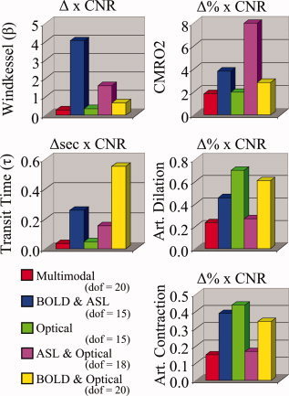
Variance inflation factors for model parameters. The lower bound on the uncertainty of each model parameter can be estimated from the variance inflation factor (Γ; described in the text). This factor determines the minimum parameter uncertainty obtainable for a fit of the fMRI, NIRS, or multimodal data. The values in this figure are normalized to the maximum response contrast per modality in order to compare across the various forms of contrast. Thus, the lower bound of the parameter uncertainty for any of the parameters can be estimated for a given contrast‐to‐noise ratio (CNR) by dividing by the CNR value (e.g., with a CNR of 20:1, the Windkessel parameter, β, can be estimated with a maximum precision of around ±0.2 StdErr using the BOLD and ASL data). The degrees‐of‐freedom (dof) for each model is given in the legend. These results are shown for a linearization about the parameter set from the model fit of the multimodal data shown in Table IV.

Table IV.

Estimation of model parameters

		Multimodal	fMRI model	Optical model	Model range
Dynamic evoked states	ΔCMRO2max [%]	16.8 ± 2.2	16.0 ± 2.3	18.3 ± 2.1	0–100 %
	(Dilation) ΔDiameter [%]	5.8 ± 1.1	5.6 ± 1.2	6.5 ± 0.7	0–90%
	(Contraction) ΔDiameter [%]	4.0 ± 2.3	3.7 ± 2.3	4.6 ± 2.1	0–90%
Static biomechanical parameters	RA(0)	0.73 ± 0.06	0.73 ± 0.04	0.74 ± 0.06	0.20–90
	β	2.39 ± 0.31	2.57 ± 0.34	1.56 ± 0.12	1.1–4
	τ [s]	1.61 ± 0.22	1.64 ± 0.27	1.14 ± 0.13	0.5–4s
	τpial [s]	2.23 ± 0.38	2.12 ± 0.68	2.21 ± 0.15	0–4s
	SaO2 [%]	95.0 ± 0.2	(95.0)	(95.0)	90–100%
	ScO2 [%]	77.6 ± 0.4	(77.6)	(77.6)	60–90%
	SvO2 [%]	63.6 ± 0.6	(63.6)	(63.6)	55–89%
Observation model	V0 [%]	5.17 ± 0.45	5.10 ± 0.52	N/a	1–10%
	ε	3.81 ± 0.02	3.75 ± 0.03	N/a	1–5.5
	[HbT]0 [μM]	100.4 ± 7.1	N/a	95.2 ± 5.8	40–140μM
	ωpial	0.56 ± 0.07	N/a	0.43 ± 0.07	0–1
	ΔFlow: ΔVolume	3.33 ± 0.12	3.40 ± 0.10	3.06 ± 0.07
	ΔFlow: ΔCMRO2	1.50 ± 0.28	1.54 ± 0.35	1.81 ± 0.26

This table shows the vascular model parameters estimated using combinations of the pulsed ASL and/or NIRS measurement data sets. In the model fit to the entire multimodal data set, the baseline oxygen saturation for the three vascular compartments was also estimated (S_aO₂‐arterial; S_cO₂‐capillary; S_vO₂‐venous). For the remaining models, these values were not fit (assumed values are given in parentheses). The 95% uncertainty bound for each parameter was estimated from Markov Chain Monte Carlo simulations using the data set (the 50% and 75% confidence intervals are also presented as box plots in Fig. 7). Model parameters are defined further in the methods section and Tables I, II, III.

Example 2: Simulation Results and Global Identifiability

The analysis of the Jacobian matrix described in our previous example indicated that the observation sets were theoretically sensitive to the parameters being estimated and thus the model was expected to be locally invertible. However, the Jacobian can only be defined about a local linearization point in nonlinear systems and such sensitivity analysis can be used to probe only the local precision of the model but not its global identifiability. Using this analysis we know that a local solution can be determined but we do not know if this solution is unique.

To investigate the uniqueness of an estimated solution, it is necessary to examine the ability of the model to correctly determine the parameter set from a global search of the parameter space. We ran forward simulations of the model using a sampling of the physiological states and parameters from within the expected physiological ranges (refer to Table III). To emulate the fMRI and NIRS experimental data, the measurements were simulated at a 2 Hz sample frequency with a random additive instrumental noise term (10:1 contrast‐to‐noise ratio to approximately match the data). We reconstructed system parameters for each simulation using the fMRI data alone, the NIRS data alone, and the full multimodality data set to explore the accuracy of the model to infer the physiological states. For all reconstructions, the Levenberg‐Marquardt minimization algorithm was initialized at a random position within the physiological range of the parameters. The same initialization was used for each modality set. Reconstructions were iterated until a set convergence criterion was met (∼10⁶ iterations that took around 6 h per model estimation). A total of 350 simulations were run for each of the three data sets.

In Figure 5A, we show parametric plots of the simulated (truth) values for the parameters used in the forward simulation against the reconstructed values obtained from each of the three data sets (NIRS only, BOLD and ASL, or NIRS, BOLD, and ASL data). The ability of a model to predict one subset of a data set (in this case the NIRS measurements) from analysis of a different subset (the fMRI data) is often used as a strategy to asses if a model has been over‐parameterized. We found that relative CMRO₂ and arterial resistance changes (ΔR _A) can be estimated accurately with both single and multi‐ modality measurement sets, consistent with the tests of local sensitivity. We examined the accuracy of the estimation of key static and response‐related parameters in the model. We found that the estimates of the Windkessel vascular reserve parameter (β) had the most variance but could still be estimated fairly accurately in spite of a slight systematic model under‐estimation bias at high values of β with the optical or fMRI only data sets. In Figure 5B, the covariance in the error of the estimates for the parameters is plotted. The lack of high correlation indicated a low interdependence between variables and minimal cross‐talk between these parameters in the model. We noted the largest cross‐talk (R ² = 0.07) between the vascular transit time through the pial‐venous compartment and the relative change in CMRO₂. We also observed negative correlation between CMRO₂ and the blood oxygen saturation parameters in the BOLD/ASL/NIRS model as also noted in [Huppert et al., 2007] (not shown). Recall that baseline oxygen saturation was not varied in the NIRS or fMRI alone models because we found these parameters were not identifiable in the reduced data sets.

Figure 5.

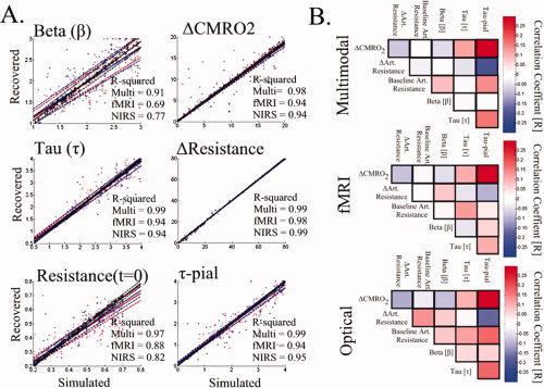
Examination of global parameter identifiability. In Panel (A), we show the results from 350 simulations of the model. fMRI and NIRS measurements were simulated at a contrast‐to‐noise ratio of 10:1. The vascular parameters (refer to Table III) were estimated from the multimodal (optical and fMRI), fMRI, or optical data sets. For each plot, the simulated and recovered values are shown (black—multimodal; red—fMRI; blue—NIRS). The solid and dotted lines show a linear regression and 95% confidence bounds. The R‐squared (R ²) values for these regressions are shown within each plot. In Panel (B), we examine the cross‐talk between each parameter by looking at the cross‐correlation (Pearson correlation coefficients) of the error in the parameter (normalized error = [recovered‐simulated]/simulated).

Example 3: Estimating Relative CMRO₂ Changes From Empirical Measurements

As a final example of the inverse procedure for our vascular model, the model was used to analyze empirical measurements of hemodynamic changes in the human motor cortex following a 2‐s finger‐tapping task. To examine the estimate of the CMRO₂ changes and other model parameters given in Table III, the model was first fit using the combined NIRS, ASL, and BOLD data set. The values of baseline blood oxygen saturation from the model fit to the full data set was then fixed and the model was applied to the ASL and BOLD data and finally to the NIRS only data.

The fits of the fMRI only and NIRS only data sets closely predicted the NIRS and fMRI data, respectively as shown in Figure 6. The 75% confidence bounds for the model fit to each measurement and the model predictions of the opposing measurement set are shown as dotted lines in Figure 6. To verify that the results of the model fit were independent of the initial position of the Levenberg‐Marquardt algorithm, we repeated the minimization for different initial seed positions (see Fig. 7). The model fit using the group‐averaged response curves was consistent with the mean of the fits to the five individual subjects (see Fig. 7). Inter‐subject variations in the parameter estimates were observed, but remained consistent whether the reduced or full data sets were used in the fitting. The values of the estimated parameters and uncertainties are given in Table IV. In Figure 7, we graphically present the estimates for the key model parameters and uncertainties for both the group and individual subject analysis. The estimated dynamic changes in arterial diameter and CMRO₂ are shown in Figure 8.

Figure 6.

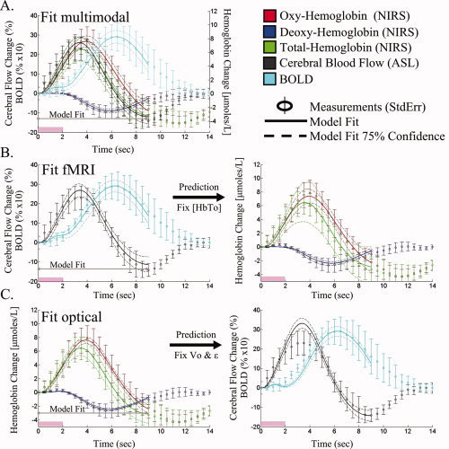
Model fit of empirical data. The vascular model was independently fit to the multimodal (Panel A), pulsed ASL and BOLD measurements (Panel B), and NIRS measurements (Panel C). Based on the parameters estimated from the model fit to one data set (i.e., fMRI alone), the remaining data (i.e., NIRS) can be predicted. These model predictions are presented for the fMRI and optical data in Rows B and C. The error bars on the data measurements (open circles) show the standard error from the group average of the five subjects. The model predictions and 75% confidence bounds are shown as solid and dashed lines in each plot. The data from 0 to 9 s was used in the model fitting procedure.

Figure 7.

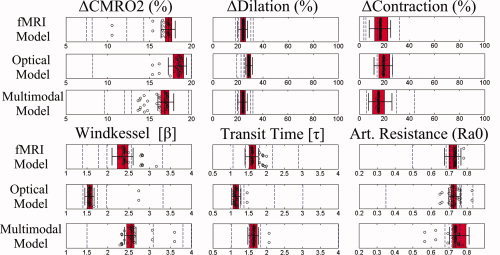
Parameter accuracy. The mean and uncertainties in the parameter estimates are illustrated using box and whisker plots to show the median (vertical line), 50% (box edges), and 75% (whiskers) percentile confidence bounds for each estimated parameter for the model fits to the group averaged data (N = 5). The results are shown for the model fits to the fMRI‐BOLD/ASL data alone, optical NIRS data alone; and multimodal BOLD/ASL/NIRS data sets. The open circles represent the fitted model parameters from variation of the initial starting position of the LM algorithm used in the analysis of the group averaged data (from variations of the extrema of the parameter bounds given in Table III). In addition, the dotted vertical lines show the mean estimates for each of the five individual subjects fit using the same model.

Figure 8.

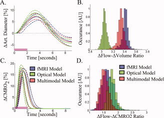
Dynamic CMRO₂ and arterial diameter changes. The dynamic changes in arterial diameter (inversely related to resistance changes) and CMRO₂ are shown in Panels (A) and (C), respectively. The solid and dotted lines show the most probable and 75% confidence intervals for the time‐courses estimated from the multimodal, fMRI, and optical data sets. Panel (B) shows the histogram of the ratio of maximum flow to volume changes recovered from the Markov Chain Monte Carlo process. In Panel (D), the flow‐consumption ratio is shown for the three data sets.

Calculated Baseline Physiological Properties

Based on the values of the estimated biomechanical parameters presented in Table IV, several additional physiological quantities can be determined and are presented in Table V. Importantly, the vascular transit time and the vascular volume fraction, needed to scale the BOLD signal were both precisely determined. Vascular volume fraction, in units of milliliters of blood per milliliter of tissue, is easily converted to blood volume, in units of milliliters of blood per 100 g of tissue, given the approximate density of brain tissue (1.04 g/ml [DiResta et al., 1991]). This baseline blood volume divided by the vascular transit time provides an estimate of baseline blood flow. Likewise, baseline CMRO₂ can be calculated from the baseline blood flow and oxygen saturation within the venous compartment. We were able to precisely estimate the venous oxygen saturation only in the model using the combined fMRI and NIRS data and we found that this estimation was not as accurate using only the fMRI only data. Thus, we fixed the value of baseline vascular oxygen saturations in the model estimates using the fMRI only or NIRS only data. Prior studies have noted that the oxygen extraction fraction varies only a few percent between different regions of the brain and this justifies constraining the range of expected cerebral venous oxygen saturation to the range of 60% ± 9% based on previous measurements in the healthy adult brain [He and Yablonskiy, 2007; Raichle et al., 2001]. The estimated baseline blood volume, blood flow, and oxygen consumption using different combinations of fMRI and NIRS data are shown in Table V. Although we assumed a value for the resting oxygen extraction in the fMRI‐only and NIRS‐only models, we found that the estimate of baseline blood flow and oxygen consumption based on the estimated scaling parameters and vascular transit time from the fMRI data alone was consistent with the estimate from the NIRS alone fit and also with the combined fMRI and NIRS fit. The values of the estimated baseline physiology for the group data and the mean of the results from the five individual subjects are presented in Table V.

Table V.

Estimates of baseline physiological parameters

		Group results	Subject A	Subject B	Subject C	Subject D	Subject E	Mean of individual subjects
Multimodal	Blood flow (ml/100/min)	82 ± 4	50	91	91	93	98	85 ± 18
	Blood Volume (ml/100g)	5.2 ± 0.2	3.2	7.5	6.3	4.8	7.5	5.8 ± 1.7
	Total Hemoglobin (μM)	100 ± 2	133	60	131	110	100	107 ± 26
	Hemoglobin content (g Hg/dl)	12.5 ± 0.1	27	5.2	13.4	14.7	8.6	13.8 ± 7.4
	Oxygen delivery (ml O2/100g/min)	14.2 ± 0.6	8.5	15.7	15.6	16	16.7	14.5 ± 3.0
	Oxygen extraction (OEF)	36.6 ± 0.5	44	48	30	34	37	38 ± 7
	CMRO2 (ml O2/100g/min)	5.2 ± 0.2	3.8	7.4	4.6	5.5	6.1	5.5 ± 1.26
	%CMRO2 (%)	16.8 ± 0.6	12.3	8.1	7.4	14.3	20	12.4 ± 4.6
	Flow: Consumption (%:%)	1.5 ± 0.6	1.6	2.6	3.1	2.1	1.9	2.2 ± 0.5
fMRI Model	Blood flow (ml/100/min)	84 ± 4	80	55	82	211	62	98 ± 57
	Blood Volume (ml/100g)	5.1 ± 0.2	3.6	7.5	5.1	6.3	7.2	5.9 ± 1.4
	Total Hemoglobin (μM)	100 ± 4	69	145	98	122	139	115 ± 28
	Hemoglobin content (g Hg/dl)	(12.5) Fixed	—	—	—	—	—	—
	Oxygen delivery (ml O2/100g/min)	14.7 ± 0.8	14	9.6	14.2	36.7	10.8	17 ± 10.0
	Oxygen extraction (OEF)	(36.6) Fixed	—	—	—	—	—	—
	CMRO2 (ml O2/100g/min)	5.3 ± 0.3	6.3	4.7	4.4	13.1	4.1	6.5 ± 3.4
	%CMRO2 (%)	16 ± 0.7	12	5	9.6	19.6	12.8	11.8 ± 4.8
	Flow: Consumption (%:%)	1.5 ± 0.1	1.4	3.8	2.4	1.9	3	2.5 ± 0.8
NIRS Model	Blood flow (ml/100/min)	93 ± 3	113	98	55	103	83	90 ± 20
	Blood Volume (ml/100g)	5.2 ± 0.1	6.7	5.2	5.2	5.2	5.2	5.5 ± 0.6
	Total Hemoglobin (μM)	92 ± 2	130	140	92	115	113	118 ± 16
	Hemoglobin content (g Hg/dl)	(12.5) Fixed	—	—	—	—	—	—
	Oxygen delivery (ml O2/100g/min)	14.8 ± 0.4	19.2	16.7	9.3	17.5	14.1	15.4 ± 3.4
	Oxygen extraction (OEF)	(36.6) Fixed	—	—	—	—	—	—
	CMRO2 (ml O2/100g/min)	5.4 ± 0.1	6.7	5.8	3.3	6.1	5	5.4 ± 1.2
	%CMRO2 (%)	18.6 ± 0.6	18.3	20	5	8.2	20	14.3 ± 6.4
	Flow: Consumption (%:%)	1.8 ± 0.1	1.5	0.5	4.3	3.4	1.8	2.3 ± 1.4

Based on the estimates of the biomechanical parameters, such as vascular transit time, oxygen saturation, and vascular volume fraction, the baseline volume, flow, and oxygen consumption can be estimated as described in (Huppert, et al. 2007). In this table recovered baseline physiological parameters are given for the model analysis of the group‐averaged response, the individual subject results, and for the average individual subject data. The values given in parentheses indicate values not fit in the models. The errors represent the 95% confidence bounds for the group analysis and standard deviations from the five individual analyses. In the case of the per subject analysis, intra‐subject variability was larger then the inter‐subject uncertainties.

DISCUSSION

Measured hemodynamic responses are the net result of the competing effects of an increased metabolic demand for oxygen and an increased supply of oxygen transported by hemoglobin through the flow‐inducing response. However, the role of variable baseline physiology and vascular biomechanical properties in the interpretation and reproducibility in the measurements of these responses has been largely under‐appreciated. In this work, we have introduced an inverse model for the analysis of multimodal hemodynamic data which depicts how baseline physiology and vascular structure affect the relative magnitudes and temporal dynamics of evoked signals. Although our model is similar to previously published models of the vascular system (reviewed in [Buxton et al., 2004]), our approach focuses on the dynamics and relative timing differences observed between multimodal measurements rather than the absolute magnitude of such signals. This allows us to characterize of the vascular properties more accurately by considering the interrelated dynamics of multimodal measurements in addition to the changes in absolute magnitude. The vascular and oxygen transport phenomena are considered simultaneously in this work, which creates a unified multimodal model that enables incorporation of both measurements of blood flow and oxygenation changes into a single and self‐consistent description of the underlying physiology. In this way, we demonstrate that BOLD signals can indirectly add information about both the flow‐volume relationship and CMRO₂ changes. We suggest that it is possible to infer blood volume changes from measurements of blood flow (ASL) and BOLD alone but note that these estimates are subject to the assumption of baseline values for oxygen extraction from the vascular compartments. Similarly, we report that blood flow changes can be inferred using measurements of blood volume and oxygen saturation changes alone (i.e., NIRS measurements). The calculated estimates of CMRO₂ and arterial resistance changes were largely consistent with those obtained when we used the full complementary set of fMRI and NIRS information.

Physiological Relevance of Estimated Model Parameters

Because the estimation of the model parameters was restricted to physiological ranges based on previous literature, it is expected that the parameter values estimated from the data are also consistent with this literature. The estimate of the Windkessel vascular reserve parameter (β) is consistent with values estimated from evoked responses found in [Jones et al., 2002; Mandeville et al., 1999b; Wu et al., 2002; Zheng et al., 2005] and in approximate agreement with the steady‐state flow‐volume relationship [Grubb et al., 1974]. Our estimated total mean vascular transit time (including pial vein) (τ = 3.3–3.8 s) is consistent with cortical gray matter values measured with dynamic susceptibility contrast‐enhanced MRI methods (DSC‐MRI) (τ = 1.2–6.9 s as compiled in [Ibaraki et al., 2006]) and previously applied to modeling the BOLD signal [Buxton et al., 2004].

We found that secondary calculations of physiological values based on the estimated parameters were also consistent with previous literature. This is further validation of our model because our analysis did not explicitly impose this consistency. For instance, while there are physiological bounds on the magnitude of both flow and consumption changes, there is a much weaker constraint on the ratio of flow to consumption changes. Our estimated ratios of peak blood flow to peak blood volume changes of 3.0–3.4 (Table III) were consistent with previous literature values of 2–4 [Huppert et al., 2007; Jones et al., 2002; Mandeville et al., 1999a; Martin et al., 2006; Wu et al., 2002]. The determined values of the flow‐to‐oxygen consumption ratio between 1.5:1 and 1.8:1 is also consistent with literature measuring these changes in comparable experiments where values of 1.5:1–3:1 have been reported in studies using fMRI [Boas et al., 2003; Dunn et al., 2005; Hoge et al., 1999; Kastrup et al., 2002] and higher ratios of 5–6 have been reported in PET studies [Fox and Raichle, 1986]. Although our estimated flow: consumption ratio is in the range of previous literature values, our estimates that utilize the ASL data were somewhat lower than the average value from the fMRI literature (∼2:1). We hypothesize that this may be a result of an unaccounted partial‐volume error in the ASL measurements arising from our defined region‐of‐interest and require further investigation. This underestimation of flow is further supported by the higher predicted flow changes from the model fit of the NIRS data set (see Fig. 6). In the ASL model, the ASL measurements were considered direct measurements of the relative flow changes and no additional scaling parameters were applied unlike the BOLD and NIRS measurements where calibration factors were estimated. We note, however, that fitting a scaling factor on both the ASL and BOLD signals may give rise to a nonunique estimation of CMRO₂ changes and baseline CMRO₂ from the ASL and BOLD only data set. The same does not apply to parameter estimation with the NIRS only data set because only one partial volume term was applied to scale oxy‐, deoxy‐, and total‐hemoglobin measurements. The value of the NIRS scaling factor does not change the ratio of hemoglobin changes (i.e., the peak oxy‐/deoxy‐ hemoglobin changes normalized to the peak total‐hemoglobin change) which is the relevant measure giving sensitivity to β and τ.

Estimates of Baseline Physiology

The estimates of baseline volume, flow, and CMRO₂, were consistent between the three dataset combinations used in the model fitting procedure (Table V). The estimate of baseline blood flow from the three data sets was 86 ml/100 g/min (mean) [range 82–93 ml/100 g/min]. Previously reported values of baseline blood flow in human cortex range from 80 to 100 ml/100 g/min in gray matter and ∼20 ml/100 g/min in white matter as measured using positron emission tomography (PET) (reviewed in [Coles, 2006; Ito et al., 2005]). Our estimates derived from evoked changes represent gray matter estimates of flow, volume, and CMRO₂. This explains why our estimates of blood flow are higher than the reported values that average gray and white matter (e.g., ∼44 ml/100 g/min from data complied in [Ito et al., 2005]).

Our estimate of baseline oxygen extraction determined from the combined BOLD, ASL, and NIRS data set was 36.6% ± 0.2%. This value is consistent with values reported in the literature of 35–43% from PET [Diringer et al., 2000; Raichle et al., 2001] and quantitative BOLD‐fMRI 38% ± 5% [He and Yablonskiy, 2007]. In the fMRI only and NIRS only models, the value of oxygen extraction was assumed based on the value obtained from the full model fit. The additional estimation of this parameter introduced considerably more uncertainty in the recovered value of CMRO₂ from these models. We consider the assumption of oxygen saturation in these models reasonable given that previous studies have demonstrated fairly small ranges for these values in normal, healthy populations. However, this assumption poses a potential source of systematic error for the application of our model to atypical subject populations.

Lastly, we estimated baseline cerebral oxygen consumption (CMRO₂). Our estimate of 5.2 ml O₂/100 g/min (mean) [range 5.2–5.4 ml O₂/100 g/min] is higher than reported values of 3.3 ± 0.5 ml O₂/100 g/min [Ito et al., 2005]. However, the values reported in these PET studies are based on flow measurements that represent the average of both gray and white matter values. Baseline CMRO₂ in gray matter is estimated to be ∼3.5–8 ml O₂/100 g/min using the literature ranges for gray matter blood flow, oxygen extraction, and hemoglobin content referred earlier.

Advantages of the Bottom‐Up Model

Our model used a curve‐fitting approach to estimate the underlying changes of CMRO₂ and arterial resistance. The use of such an inverse model allows us to incorporate our multimodal data into a unified estimate of the underlying physiology. In contrast to our approach, most previous formulations of vascular models have been built around a top‐down (or deductive) approach where CMRO₂ changes are estimated from the set of hemodynamic measurements. Because deductive models calculate CMRO₂ changes directly from measurements, the results directly reflect the quality of the data used. In such models, CMRO₂ changes can be recovered only at the lowest spatial and temporal resolutions of the data used. In addition, the error in the estimate of CMRO₂ is compounded by the errors in multiple measurements and the resulting estimates generally have errors greater than the noisiest measurements used.

In an inductive framework, measurements are forward‐modeled from changes in the underlying states (i.e., arterial resistance and CMRO₂). The estimate of the underlying states requires the solution of an inverse problem, which is more computationally intensive than the equations used in the deductive approach. However, the distinct advantage of the inductive approach is that model inversion may be possible with limited sets of observations (as in the fMRI alone analysis) and redundant information can be fused into estimates that maximize the joint probability of all observations (as in the full multimodal analysis). The inductive framework predicts all possible observations, not all of which are necessarily measured thus allowing the use of a smaller subset of possible observations to estimate the parameters in the model. Additionally, the inductive model may be used to take advantage of advanced state‐space estimation techniques, which are particularly useful for hidden‐variable or under‐determined problems. Several methods have been described to solve problems in this framework, such as the Kalman filter for dynamically variant systems. In this model, we use a time‐invariant approach, but recognize that advanced techniques could provide additional advantages in future work. Lastly, the model setup described has the advantage of providing a mechanism by which multimodality information can be fused within a Bayesian framework by incorporating statistical error of each measurement and the corresponding observation model for each modality. Recently several similar inductive models have been applied to interpretation of fMRI data [Deneux and Faugeras, 2006; Friston, 2002] and the fusion of fMRI and EEG data [Riera et al., 2005].

Model Assumptions and Future Extensions

The vascular model we have described is a simplified approximation of the complex behavior of the cerebral system. Therefore, we must be cautious in the physiological interpretation of such model‐based results and identify how they may be affected by the assumptions made. These approximations must be tested and either confirmed or refined based on future human and invasive animal model studies. We believe that this model will provide a mechanism to develop hypotheses which may facilitate future testing of the consistency of these model assumptions with experimental evidence. On the basis of our model, we can make predictions about how the evoked response is expected to change under different conditions, for example hyperemia. Testing these hypotheses can provide a means to examine the validity of our assumptions and provide corrections if necessary. We believe that the development of a unified model to allow us to examine measurements from a variety of different imaging modalities, experimental conditions, and animal models including both human (as described this work) and invasive small animal studies [Huppert et al., 2007], is important to improving the understanding of cerebral mechanisms in future work.

In our current model, the estimation of CMRO₂ from ASL and BOLD data assumes the values of the relative volume fraction and the oxygen saturation of each vascular compartment. The baseline volume fraction of the arterial, capillary, and venous compartments used in this study was assumed to be 25, 15, and 60%, respectively [Duong and Kim, 2000]. This assumption may affect the accuracy of the BOLD calibration and estimated CMRO₂ changes to the extent of the variability of these volume fractions between different cortical regions of the brain.

Although the dynamics of the fMRI response is sensitive to the baseline oxygen extraction, we found that the additional fitting of the baseline oxygen saturations of each vascular compartment in the fMRI only or optical only models created considerable uncertainty in the estimation of relative CMRO₂. We found that the most probable value of relative CMRO₂ estimated from the fMRI data was consistent whether or not the oxygen saturation parameters were allowed to vary in the model (19% ± 6% maximum rCMRO₂ when fitting for oxygen saturation), and the uncertainty of this magnitude was much larger unless oxygen saturation was assumed. In previous work, Raichle et al. have suggested that there was little spatial variation in the oxygen extraction fraction across the normal healthy adult brain [Raichle et al., 2001] and, thus, we believe that it is reasonable to use an a priori assumption of oxygen extraction values to help better constrain model. The validity of this assumption, however, is suspect in pathological cases. We note that the oxygen saturation of each vascular compartment could be estimated when the full set of blood flow, volume, and oxygen saturation (or BOLD) changes were included in the model.

Furthermore, the estimates of absolute functional and baseline parameters rely on the quantitative accuracy of the measurement methods which in turn depends on uncorrected partial volume errors. In this work, we have neglected partial volume errors of the fMRI methods. For the optical data, partial volume effects were corrected using the anatomical information from MRI [Huppert et al., 2006a]. However, we note that the accuracy of this correction depends on the accuracy of the model of light propagation in the tissue. Uncertainty in the estimated baseline blood volume, flow, and CMRO₂ is linearly dependent on any systematic errors in the partial volume correction. We found that the estimates of relative changes in CMRO₂, blood flow, or volume are largely unaffected by partial volume errors because these parameters are normalized within the model and are affected only by uncertainties in the temporal characteristics and relative magnitudes of the hemodynamic signals.

A final limitation of our model is its numerical complexity and the extensive computational power needed to perform the model inversion and estimation of parameters. Because of this complexity, we currently limited the analysis to only one or a few regions‐of‐interest within the brain. Systematic biases may thus have been introduced due to (i) the choice of the region‐of‐interest, (ii) varying spatial resolution of the optical and fMRI measurements, and (iii) the potential for displacement of the locations of different functional contrast types due to the underlying arterial and venous spatial structure [Huppert et al., 2006a]. In future work, this vascular model can be extended to incorporate a more accurate forward tomography model of the optical measurements which may allow the reconstruction of CMRO₂ and flow volume images. It should be noted that this will require of the use of more efficient computational methods within future work in order to overcome the high dimensionality of the nonlinear imaging problem.

CONCLUSIONS

Hemodynamic changes are influenced by both evoked metabolic and vascular response, but are also sensitive to the biomechanical, structural, and physiological state of the brain. By using multimodal methods to investigate these changes and, in particular, by examining the dynamic characteristics and inter‐relationships between different measurement types, we have found that multimodal fMRI measurements may be used to examine some of the underlying properties of the brain. We have illustrated how our dynamic vascular model may be used to obtain estimates of some of the underlying physiological properties of the brain based on curve‐fitting techniques and high‐temporal resolution functional signals. Further confirmation and validation of our approach would provide an important new approach for estimating evoked changes in cerebral oxygen metabolism with fMRI without the need to calibrate the BOLD signal with hypercapnia or assume a flow‐volume relationship.

REFERENCES

- Bamber D,van Santen JP ( 2000): How to assess a model's testability and identifiability. J Math Psychol 44: 20–40. [DOI] [PubMed] [Google Scholar]
- Belliveau JW,Kennedy DN Jr,McKinstry RC,Buchbinder BR,Weisskoff RM,Cohen MS,Vevea JM,Brady TJ,Rosen BR ( 1991): Functional mapping of the human visual cortex by magnetic resonance imaging. Science 254: 716–719. [DOI] [PubMed] [Google Scholar]
- Boas DA,Strangman G,Culver JP,Hoge RD,Jasdzewski G,Poldrack RA,Rosen BR,Mandeville JB ( 2003): Can the cerebral metabolic rate of oxygen be estimated with near‐infrared spectroscopy? Phys Med Biol 48: 2405–2418. [DOI] [PubMed] [Google Scholar]
- Boxerman JL,Bandettini PA,Kwong KK,Baker JR,Davis TL,Rosen BR,Weisskoff RM ( 1995): The intravascular contribution to fMRI signal change: Monte Carlo modeling and diffusion‐weighted studies in vivo. Magn Reson Med 34: 4–10. [DOI] [PubMed] [Google Scholar]
- Buxton RB,Uludag K,Dubowitz DJ,Liu TT ( 2004): Modeling the hemodynamic response to brain activation. Neuroimage 23( Suppl. 1): S220–S233. [DOI] [PubMed] [Google Scholar]
- Cannestra AF,Pouratian N,Shomer MH,Toga AW ( 1998): Refractory periods observed by intrinsic signal and fluorescent dye imaging. J Neurophysiol 80: 1522–1532. [DOI] [PubMed] [Google Scholar]
- Cohen ER,Ugurbil K,Kim SG ( 2002): Effect of basal conditions on the magnitude and dynamics of the blood oxygenation level‐dependent fMRI response. J Cereb Blood Flow Metab 22: 1042–1053. [DOI] [PubMed] [Google Scholar]
- Coles JP ( 2006): Imaging of cerebral blood flow and metabolism. Curr Opin Anaesthesiol 19: 473–480. [DOI] [PubMed] [Google Scholar]
- Cooper CE,Elwell CE,Meek JH,Matcher SJ,Wyatt JS,Cope M,Delpy DT ( 1996): The noninvasive measurement of absolute cerebral deoxyhemoglobin concentration and mean optical path length in the neonatal brain by second derivative near infrared spectroscopy. Pediatr Res 39: 32–38. [DOI] [PubMed] [Google Scholar]
- Cope M,Delpy DT,Reynolds EO,Wray S,Wyatt J,van der Zee P ( 1988): Methods of quantitating cerebral near infrared spectroscopy data. Adv Exp Med Biol 222: 183–189. [DOI] [PubMed] [Google Scholar]
- Cox RW,Jesmanowicz A ( 1999): Real‐time 3D image registration for functional MRI. Magn Reson Med 42: 1014–1018. [DOI] [PubMed] [Google Scholar]
- Davis TL,Kwong KK,Weisskoff RM,Rosen BR ( 1998): Calibrated functional MRI: Mapping the dynamics of oxidative metabolism. Proc Natl Acad Sci USA 95: 1834–1839. [DOI] [PMC free article] [PubMed] [Google Scholar]
- Delpy DT,Cope M,van der Zee P,Arridge S,Wray S,Wyatt J ( 1988): Estimation of optical pathlength through tissue from direct time of flight measurement. Phys Med Biol 33: 1433–1442. [DOI] [PubMed] [Google Scholar]
- Deneux T,Faugeras O ( 2006): Using nonlinear models in fMRI data analysis: Model selection and activation detection. Neuroimage 32: 1669–1689. [DOI] [PubMed] [Google Scholar]
- DiResta GR,Lee JB,Arbit E ( 1991): Measurement of brain tissue specific gravity using pycnometry. J Neurosci Methods 39: 245–251. [DOI] [PubMed] [Google Scholar]
- Diringer MN,Yundt K,Videen TO,Adams RE,Zazulia AR,Deibert E,Aiyagari V,Dacey RG Jr,Grubb RL Jr,Powers WJ ( 2000): No reduction in cerebral metabolism as a result of early moderate hyperventilation following severe traumatic brain injury. J Neurosurg 92: 7–13. [DOI] [PubMed] [Google Scholar]
- Duncan A,Meek JH,Clemence M,Elwell CE,Tyszczuk L,Cope M,Delpy DT ( 1995): Optical pathlength measurements on adult head, calf and forearm and the head of the newborn infant using phase resolved optical spectroscopy. Phys Med Biol 40: 295–304. [DOI] [PubMed] [Google Scholar]
- Dunn AK,Devor A,Dale AM,Boas DA ( 2005): Spatial extent of oxygen metabolism and hemodynamic changes during functional activation of the rat somatosensory cortex. Neuroimage 27: 279–290. [DOI] [PubMed] [Google Scholar]
- Duong TQ,Kim SG ( 2000): In vivo MR measurements of regional arterial and venous blood volume fractions in intact rat brain. Magn Reson Med 43: 393–402. [DOI] [PubMed] [Google Scholar]
- Fox PT,Raichle ME ( 1986): Focal physiological uncoupling of cerebral blood flow and oxidative metabolism during somatosensory stimulation in human subjects. Proc Natl Acad Sci USA 83: 1140–1144. [DOI] [PMC free article] [PubMed] [Google Scholar]
- Friston KJ ( 2002): Bayesian estimation of dynamical systems: An application to fMRI. Neuroimage 16: 513–530. [DOI] [PubMed] [Google Scholar]
- Grubb RL Jr,Raichle ME,Eichling JO,Ter‐Pogossian MM ( 1974): The effects of changes in PaCO2 on cerebral blood volume, blood flow, and vascular mean transit time. Stroke 5: 630–639. [DOI] [PubMed] [Google Scholar]
- Habler OP,Messmer KF ( 1997): The physiology of oxygen transport. Transfus Sci 18: 425–435. [DOI] [PubMed] [Google Scholar]
- He X,Yablonskiy DA ( 2007): Quantitative BOLD: Mapping of human cerebral deoxygenated blood volume and oxygen extraction fraction: Default state. Magn Reson Med 57: 115–126. [DOI] [PMC free article] [PubMed] [Google Scholar]
- Herman P,Trubel HK,Hyder F ( 2006): A multiparametric assessment of oxygen efflux from the brain. J Cereb Blood Flow Metab 26: 79–91. [DOI] [PubMed] [Google Scholar]
- Hiraoka M,Firbank M,Essenpreis M,Cope M,Arridge SR,van der Zee P,Delpy DT ( 1993): A Monte Carlo investigation of optical pathlength in inhomogeneous tissue and its application to near‐infrared spectroscopy. Phys Med Biol 38: 1859–1876. [DOI] [PubMed] [Google Scholar]
- Hoge RD,Atkinson J,Gill B,Crelier GR,Marrett S,Pike GB ( 1999): Stimulus‐dependent BOLD and perfusion dynamics in human V1. Neuroimage 9 (Part 1): 573–585. [DOI] [PubMed] [Google Scholar]
- Huppert TJ ( 2007): The Hemodynamic Inference of Cerebral Oxygen Metabolism, PhD Thesis. Boston, MA: Harvard University. p 503.
- Huppert T,Hoge RD,Dale AM,Franceschini MA,Boas DA ( 2006a): A quantitative spatial comparison of diffuse optical imaging with BOLD‐ and ASL‐based fMRI. J Biomed Opt 11: 064018. [DOI] [PMC free article] [PubMed] [Google Scholar]
- Huppert TJ,Hoge RD,Diamond SG,Franceschini MA,Boas DA ( 2006b): A temporal comparison of BOLD, ASL, and NIRS hemodynamic responses to motor stimuli in adult humans Neuroimage 29: 368–382. [DOI] [PMC free article] [PubMed] [Google Scholar]
- Huppert TJ,Allen MS,Benav H,Jones P,Boas DA ( 2007): A multi‐compartment vascular model for inferring arteriole dilation and cerebral metabolic changes during functional activation. J Cereb Blood Flow Metab 27: 1262–1279. [DOI] [PMC free article] [PubMed] [Google Scholar]
- Ibaraki M,Ito H,Shimosegawa E,Toyoshima H,Ishigame K,Takahashi K,Kanno I,Miura S ( 2007): Cerebral vascular mean transit time in healthy humans: A comparative study with PET and dynamic susceptibility contrast‐enhanced MRI. J Cereb Blood Flow Metab 27: 404–413. [DOI] [PubMed] [Google Scholar]
- Ito H,Kanno I,Fukuda H ( 2005): Human cerebral circulation: Positron emission tomography studies. Ann Nucl Med 19: 65–74. [DOI] [PubMed] [Google Scholar]
- Jones M,Berwick J,Mayhew J ( 2002): Changes in blood flow, oxygenation, and volume following extended stimulation of rodent barrel cortex. Neuroimage 15: 474–487. [DOI] [PubMed] [Google Scholar]
- Kastrup A,Kruger G,Neumann‐Haefelin T,Glover GH,Moseley ME ( 2002): Changes of cerebral blood flow, oxygenation, and oxidative metabolism during graded motor activation. Neuroimage 15: 74–82. [DOI] [PubMed] [Google Scholar]
- Leung TS,Tachtsidis I,Smith M,Delpy DT,Elwell CE ( 2006): Measurement of the absolute optical properties and cerebral blood volume of the adult human head with hybrid differential and spatially resolved spectroscopy. Phys Med Biol 51: 703–717. [DOI] [PubMed] [Google Scholar]
- Liu H,Chance B,Hielscher AH,Jacques SL,Tittel FK ( 1995): Influence of blood vessels on the measurement of hemoglobin oxygenation as determined by time‐resolved reflectance spectroscopy. Med Phys 22: 1209–1217. [DOI] [PubMed] [Google Scholar]
- Liu TT,Behzadi Y,Restom K,Uludag K,Lu K,Buracas GT,Dubowitz DJ,Buxton RB ( 2004): Caffeine alters the temporal dynamics of the visual BOLD response. Neuroimage 23: 1402–1413. [DOI] [PubMed] [Google Scholar]
- Lu H,van Zijl PC ( 2005): Experimental measurement of extravascular parenchymal BOLD effects and tissue oxygen extraction fractions using multi‐echo VASO fMRI at 1.5 and 3.0 T. Magn Reson Med 53: 808–816. [DOI] [PubMed] [Google Scholar]
- Lu H,Donahue MJ,van Zijl PC ( 2006): Detrimental effects of BOLD signal in arterial spin labeling fMRI at high field strength. Magn Reson Med 56: 546–552. [DOI] [PubMed] [Google Scholar]
- Luh WM,Wong EC,Bandettini PA,Hyde JS ( 1999): QUIPSS II with thin‐slice TI1 periodic saturation: A method for improving accuracy of quantitative perfusion imaging using pulsed arterial spin labeling. Magn Reson Med 41: 1246–1254. [DOI] [PubMed] [Google Scholar]
- Mandeville JB,Marota JJ,Ayata C,Moskowitz MA,Weisskoff RM,Rosen BR ( 1999a): MRI measurement of the temporal evolution of relative CMRO(2) during rat forepaw stimulation. Magn Reson Med 42: 944–951. [DOI] [PubMed] [Google Scholar]
- Mandeville JB,Marota JJ,Ayata C,Zaharchuk G,Moskowitz MA,Rosen BR,Weisskoff RM ( 1999b): Evidence of a cerebrovascular postarteriole windkessel with delayed compliance. J Cereb Blood Flow Metab 19: 679–689. [DOI] [PubMed] [Google Scholar]
- Marquardt DW ( 1963): An algorithm for least‐squares estimation of nonlinear parameters. J Soc Ind Appl Math 11: 431–441. [Google Scholar]
- Martin C,Jones M,Martindale J,Mayhew J ( 2006): Haemodynamic and neural responses to hypercapnia in the awake rat. Eur J Neurosci 24: 2601–2610. [DOI] [PubMed] [Google Scholar]
- Mildner T,Norris DG,Schwarzbauer C,Wiggins CJ ( 2001): A qualitative test of the balloon model for BOLD‐based MR signal changes at 3T. Magn Reson Med 46: 891–899. [DOI] [PubMed] [Google Scholar]
- Nair DG ( 2005): About being BOLD. Brain Res Brain Res Rev 50: 229–243. [DOI] [PubMed] [Google Scholar]
- Obata T,Liu TT,Miller KL,Luh WM,Wong EC,Frank LR,Buxton RB ( 2004): Discrepancies between BOLD and flow dynamics in primary and supplementary motor areas: Application of the balloon model to the interpretation of BOLD transients. Neuroimage 21: 144–153. [DOI] [PubMed] [Google Scholar]
- Obrig H,Hirth C,Junge‐Hulsing JG,Doge C,Wolf T,Dirnagl U,Villringer A ( 1996): Cerebral oxygenation changes in response to motor stimulation. J Appl Physiol 81: 1174–1183. [DOI] [PubMed] [Google Scholar]
- Ogawa S,Lee TM,Kay AR,Tank DW ( 1990): Brain magnetic resonance imaging with contrast dependent on blood oxygenation. Proc Natl Acad Sci USA 87: 9868–9872. [DOI] [PMC free article] [PubMed] [Google Scholar]
- Raichle ME,MacLeod AM,Snyder AZ,Powers WJ,Gusnard DA,Shulman GL ( 2001): A default mode of brain function. Proc Natl Acad Sci USA 98: 676–682. [DOI] [PMC free article] [PubMed] [Google Scholar]
- Riera J,Aubert E,Iwata K,Kawashima R,Wan X,Ozaki T ( 2005): Fusing EEG and fMRI based on a bottom‐up model: Inferring activation and effective connectivity in neural masses. Philos Trans R Soc Lond B Biol Sci 360: 1025–1041. [DOI] [PMC free article] [PubMed] [Google Scholar]
- Sicard KM,Duong TQ ( 2005): Effects of hypoxia, hyperoxia, and hypercapnia on baseline and stimulus‐evoked BOLD, CBF, and CMRO2 in spontaneously breathing animals Neuroimage 25: 850–858. [DOI] [PMC free article] [PubMed] [Google Scholar]
- Villringer A,Chance B ( 1997): Non‐invasive optical spectroscopy and imaging of human brain function. Trends Neurosci 20: 435–442. [DOI] [PubMed] [Google Scholar]
- Washburn EW ( 1921): The dynamics of capillary flow. Phys Rev Lett 12: 273–283. [Google Scholar]
- Wong EC,Buxton RB,Frank LR ( 1997): Implementation of quantitative perfusion imaging techniques for functional brain mapping using pulsed arterial spin labeling. NMR Biomed 10: 237–249. [DOI] [PubMed] [Google Scholar]
- Wu G,Luo F,Li Z,Zhao X,Li SJ ( 2002): Transient relationships among BOLD, CBV, and CBF changes in rat brain as detected by functional MRI. Magn Reson Med 48: 87–93. [DOI] [PubMed] [Google Scholar]
- Yablonskiy DA,Haacke EM ( 1994): Theory of NMR signal behavior in magnetically inhomogeneous tissues: The static dephasing regime. Magn Reson Med 32: 749–763. [DOI] [PubMed] [Google Scholar]
- Zheng Y,Johnston D,Berwick J,Chen D,Billings S,Mayhew J ( 2005): A three‐compartment model of the hemodynamic response and oxygen delivery to brain. Neuroimage 28: 925–939. [DOI] [PubMed] [Google Scholar]