Trichromatic reconstruction from the interleaved cone mosaic: Bayesian model and the color appearance of small spots

Abstract

Observers use a wide range of color names, including white, to describe monochromatic flashes with a retinal size comparable to that of a single cone. We model such data as a consequence of information loss arising from trichromatic sampling. The model starts with the simulated responses of the individual L, M, and S cones actually present in the cone mosaic and uses these to reconstruct the L-, M-, and S-cone signals that were present at every image location. We incorporate the optics and the mosaic topography of individual observers, as well as the spatio-chromatic statistics of natural images. We simulated the experiment of H. Hofer, B. Singer, & D. R. Williams (2005) and predicted the color name on each simulated trial from the average chromaticity of the spot reconstructed by our model. Broad features of the data across observers emerged naturally as a consequence of the measured individual variation in the relative numbers of L, M, and S cones. The model’s output is also consistent with the appearance of larger spots and of sinusoidal contrast modulations. Finally, the model makes testable predictions for future experiments that study how color naming varies with the fine structure of the retinal mosaic.

Introduction

Trichromatic sampling

Human color vision is mediated by three classes of retinal cones, the L, M, and S cones. That there are only three classes means that color vision is trichromatic: Two lights with distinct spectra that produce the same photopigment isomerization rates in all three classes will be indistinguishable to the visual system. Such lights are referred to as metamers. Metamerism is a special case of aliasing, where two physically distinct images produce the same responses in an extended array of photoreceptors.

Standard treatments of human trichromacy (e.g., Brainard, 1995; Kaiser & Boynton, 1996; Wandell, 1995; Wyszecki & Stiles, 1982) generally neglect the interleaved structure of the retinal cone mosaic. These treatments of trichromacy break down, however, at fine spatial scales. This is because there is at most one cone sensing light at any particular location, so that two retinal images that differ in both their spatial and spectral properties can be aliases of one another (Brainard, 1994; Brainard & Williams, 1993; Williams, Sekiguchi, Haake, Brainard, & Packer, 1991). This idea is illustrated in Figure 1.

Figure 1.

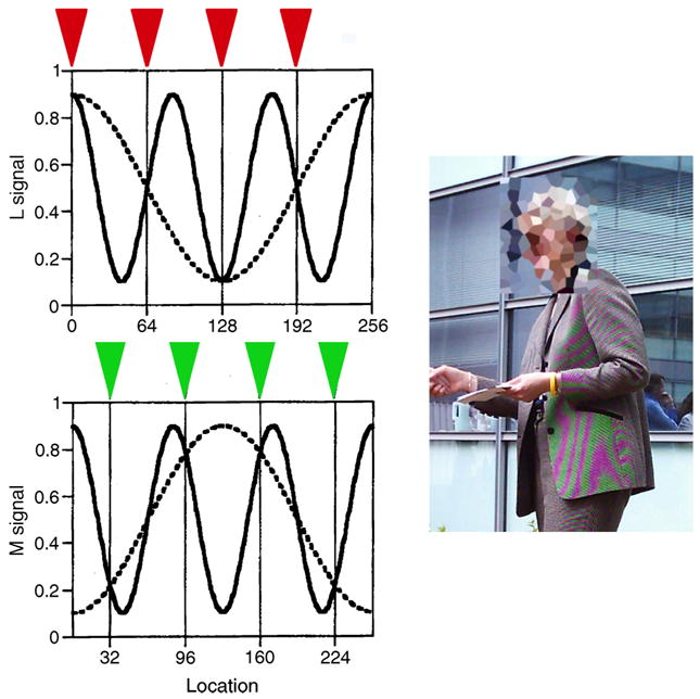
Aliasing can occur with interleaved mosaics. (Left panel) The figure illustrates how two physically distinct signals that vary spatially and spectrally can produce the same responses in an interleaved mosaic of cones. For simplicity, the example is for a single spatial dimension and a retina containing only L and M cones. Once the spectral sensitivities of the cones are taken into account, the spatio-spectral image is described by the L- and M-cone isomerization rates at each spatial location (L and M signals). Two distinct images are represented in the figure, one by the solid line in both plots and one by the dashed line in both plots. The solid line shows an image consisting of a 3 cycle per image isochromatic grating in which L and M signals vary together. The dashed line shows a 1 cycle per image red/green grating in which L and M signals vary in counterphase. These images are sensed by a mosaic consisting of 8 cones, 4 L cones and 4 M cones, arranged in a regular interleaved fashion. Locations of cones are shown as triangles at the top of each plot. The two images have the same L-cone signal at each location where there is an L cone, and the same M-cone signal at each location where there is an M cone. Thus, the two images are aliases, as they produce the same responses in each retinal cone receptor. Note that this aliasing occurs even though both patterns have spatial frequencies below the 4 cycle per image Nyquist rate for the mosaic as a whole. Panel adopted from Brainard (1994). (Right panel) Aliasing of the sort shown in the left panels occurs in digital color imaging. Most digital cameras employ interleaved R, G, and B sensors, analogous to the interleaved cone sampling of the human retina. In the image on the right, the high-spatial frequency intensity variation of the jacket is rendered by the camera as its lower spatial frequency red/green alias. Image courtesy of J. Kraft; the face of the photographic subject has been pixelated to preserve anonymity.

The computational problem posed by interleaved mosaic design is as follows. The visual system has available the isomerization rates of one cone class at each cone location. To provide a representation of a spatially varying trichromatic signal, the visual system must reconstruct the isomerization rates of the two missing cone classes at each location. It is clear that this is an underdetermined estimation problem since direct information about the isomerizations of the two missing cone classes at each location is eliminated by interleaved sampling. How the visual system copes with the information loss is largely unknown. In this paper, we present a model of the process and compare its predictions with psychophysical data and observations.

Psychophysical data

Historically, it has been difficult to identify empirical phenomena that result from interleaved trichromatic sampling and thus allow study of the computations related to this sampling. Although aliasing of intensity variation into chromatic variation is a routine artifact in digital color imaging (see Figure 1), demonstrations of parallel phenomena in humans have been elusive. Williams et al. (1991) argued that an effect known as Brewster’s colors, wherein colored patterns can be seen on top of high-contrast isochromatic gratings, represent one such example. They suggested that the fleeting nature of the effect resulted from clever processing by the visual system. Nonetheless, the aliasing artifacts were subtle and difficult to exploit for systematic modeling.

Filling-in at the tritanopic area (e.g., Williams, MacLeod, & Hayhoe, 1981) provides another example of spatio-chromatic aliasing. Brainard and Williams (1993) showed that the perceived S-cone component of the stimulus at the tritanopic area is influenced by L- and M-cone signals, a direct empirical verification that signals from different cone classes can interact in the reconstruction algorithm used by the visual system.

Recently, Hofer, Singer, et al. (2005) reported experiments where observers named the color appearance of small flashed retinal spots. By using adaptive optics to correct the aberrations in individual observers, they were able to present spots whose retinal size was similar in scale to the acceptance aperture of single cones. Moreover, they were able to measure the spatial arrangement and classes of the cones in the same general retinal region as they presented the flashed spots. Their experiment provides an opportunity to study the reconstruction algorithm employed by the visual system, since a report of the color name of a flash that stimulates only one cone implies estimates of the signals seen by the two cone classes missing at the spot location.

Bayesian model of trichromatic reconstruction

Here we report a quantitative model of the experiment of Hofer, Singer, et al. (2005). The model is based on a Bayesian algorithm that solves the general reconstruction problem posed by interleaved spectral sampling. We implemented the algorithm using measurements of individual observer cone mosaics and optics and used simulation to evaluate the algorithm’s performance for the small spot experiment. This allowed us to compare the human data to the algorithm’s predictions in aggregate. We find that the model provides a good first-order account of the data, and that it also accounts for other color appearance phenomena. Moreover, the model makes testable predictions for the results of future experiments.

Methods

Measurements of small spot colors

The experimental procedures and results are described in detail by Hofer, Singer, et al. (2005). Briefly, an adaptive optics system was used to measure and correct for aberrations in the optics of individual observers. This enabled resolution of individual cones in acquired fundus images. Retinal densitometry performed using the adaptive optics system (Hofer, Carroll, Neitz, Neitz, & Williams, 2005; Hofer, Singer, et al., 2005; Roorda & Williams, 1999) allowed determination of the location and class (L, M, or S) of individual cones in small retinal regions at ~1° retinal eccentricity. Such regions were characterized for 5 observers, and ~12′ × ~12′ subregions of characterized mosaic for each observer are shown schematically in Figure 2. We used the mosaics shown for the computations presented here.

Figure 2.

Basic data from Hofer, Singer, et al. (2005). (Top panels) Schematics of retinal mosaics used for the 5 observers. These are subsets of the full regions characterized for each observer. For each observer, the imaging and densitometry data were insufficient to assign a class or exact location to some cones. These parameters were filled in according to the procedure described by Hofer, Singer, et al. (2005). In the schematics, L cones are colored red, M cones green, and S cones blue. L:M ratios of mosaics used: HS 1:3.1; YY 1.2:1; AP 1.3:1; MD 1.6:1, BS, 14.7:1. These ratios differ slightly from those provided by Hofer, Singer, et al. because here we report the ratios for the subregions of the mosaic used in our model rather than the ratio from the larger mosaic regions studied by Hofer, Singer, et al. (Bottom panel) The bar plot shows the color naming data for each observer. Each bar represents performance for one observer. The proportion of the bar depicted in each color provides the percent of the corresponding color name used by that observer, for detected spots that were namable. From bottom to top of each bar, the possible color names are red, orange, yellow, yellow-green, green, blue-green, blue, purple, and white. Data averaged over 500-, 550-, and 600-nm spots and correspond to the intensity of 50% seeing for each observer. Data replotted from Hofer, Singer, et al. (2005).

The adaptive optics system was used to briefly present small monochromatic spots (~0.3-minute full-width at half-maximum retinal size, <4 ms duration) at the retinal region where the mosaic had been characterized. The location of each spot within the region varied from trial-to-trial because of fixational eye movements, so it was not possible to know the exact location of each flashed spot. Spots were presented at near threshold intensities, determined individually for each observer, and observers named the color of each seen spot. Observers chose the color name from the set red, orange, yellow, yellow-green, green, blue-green, blue, purple, or white. Some seen spots were also judged unnamable by observers. This is an interesting aspect of the data that we have not attempted to account for. Not all observers employed all available color names.

The bottom panel of Figure 2 shows the color naming performance of all 5 observers averaged over 500-, 550-, and 600-nm spots. Several features of the data are noteworthy. First, observers required a wide range of color names to describe their experience; all observers employed at least 5 color names across the experimental conditions studied. Second, all observers described a nontrivial percentage of spots as white. Third, there was substantial individual variation in the naming data. For example, the percentage of spots named white was smallest for observers with roughly equal numbers of L and M cones and largest for observers with either L-cone-dominated or M-cone-dominated mosaics.

Model structure

Overview

Figure 3 shows the steps in the model calculation. In the treatment here, various numerical quantities are given symbolic names. Table 1 provides a summary of the notation and typical values.

Figure 3.

Overview of model structure. The first step was to simulate the presentation of small monochromatic spots. For each presentation, we then calculated the retinal image that would be produced by the spot and from this the array of cone responses. A model of spot detection was implemented, so that color names were evaluated for spots predicted as seen. The cone responses for seen spots were used as the input to the Bayesian reconstruction algorithm, which produced a reconstructed image for each seen spot. The chromaticity of the reconstructed spot was used to predict its color name.

Table 1.

Symbols and typical values.

Symbol	Meaning	Value
Npixel	Linear size of simulated image, pixelsa	100–101
Kimage	Size of simulated image, minutesa	11.4–12.6
Kspot	Simulated spot size, minutes	0.3
Kconeaperture	Cone aperture, minutes	0.9
xspot, yspot	Location of a particular simulated spot
Ispot	Simulated spot intensity
λspot	Simulated spot wavelength, nmb	500, 550, 600
Ncones	Number of cones in image areaa	128–216
Nneighbors	Number of cone neighbors in detection model	4
ycriterion	Criterion in detection model	10
ymeanmosaic	Vector of mean cone responses
ynoisymosaic	Vector of noisy cone responses
ypooled	Pooled cone response in detection model
p(x)	Prior over trichromatic images
p(y|x)	Likelihood of cone responses, given trichromatic image
p(x|y)	Posterior over trichromatic images, given cone responses
xestimate	Vector representing reconstructed trichromatic image
ux	Prior mean vector for trichromatic images x
Kx	Prior covariance matrix for trichromatic images x
uspace	Prior mean of spatial prior at each location	1
${\sigma }_{\text{space}}^2$	Prior variance of spatial prior at each location	0.25
ρspace	Nearest neighbor correlation of spatial prior	0.75
Nlinmod	Dimensionality used in approximation of 1-D spatial prior	20
uu′ v′	Mean of color prior in CIE u′ v′ chromaticity	[0.198, 0.472]′
${\sigma }_{u^{\prime }{v}^{\prime }}^2$	CIE u′ v′variance of color prior	0.09
κcolor	Factor relating ${\sigma }_{\text{factor}}^2$ and μfactor	4

^aNote: Range provided represents range across observers.

^bValues given represent values used across experimental conditions.

Stimulus representation

On every trial of the simulation, an N_pixel × N_pixel image representing a small monochromatic spot was created. The image corresponded to K_image × K_image minutes of arc, and the size of the simulated spot was that of the physical stimulus used in the experiment (K_spot minutes in diameter). The spot location x_spot, y_spot was chosen at random within the image, subject to the requirement that its center be at least one cone aperture diameter away from the edge of the image. The wavelength λ_spot of the simulated spots matched those used in the experiments. We specified spot intensities (I_spot) in arbitrary units and linked these to the physical spot intensities used in the experiments through a psychophysical model of spot detection (see below).

Calculation of retinal image

The retinal image is formed when the stimulus is blurred by the eye’s optics. We computed the retinal image using point spread functions calculated for each individual observer at the spot wavelength from measurements of the residual optical aberration of that subject acquired during adaptive optics correction (Hofer, Singer, et al., 2005). The adaptive optics point spread function was represented at the same pixel resolution as the image. For convenience in computing cone isomerization rates, we also incorporated blurring by the cone aperture at this stage. We assumed a Gaussian aperture for each cone, with a full-width at half-maximum of 61.5% of the nominal cone diameter (K_coneaperture, in minutes of arc).

Calculation of cone responses

Measurements of cone location and cone class for each observer, as described above, were used to sample the retinal image (see Figure 2). We used I_spot, λ_spot, and the Smith–Pokorny (DeMarco, Pokorny, & Smith, 1992; Smith & Pokorny, 1975) estimates of cone spectral sensitivities, with the function for each cone normalized to have a quantal sensitivity of one at its wavelength of maximum sensitivity, to compute the mean isomerization rate u_mean of each of the N_cones cones contained within the K_image × K_image minute mosaic. As noted above, intensities in the simulations were specified in arbitrary units, so we simply took the mean isomerization rates directly as the inner product of the spot spectrum and the normalized spectral sensitivities; coupling of intensity to the experiment was achieved through the detection model.

The mean isomerization rates were used to compute simulated isomerizations for each cone through a draw from a Poisson distribution with its mean, u_mean. We refer to the result as the cone responses. In the calculations below, it is convenient to represent the mean cone responses as an N_cones-dimensional column vector y_meanmosaic, and the responses with noise added as y_noisymosaic.

Detection model

In the experiments, observers made a yes–no judgment as to whether they saw each flash and named the color of flashes seen (or indicated that the flash was unnamable). Experiments were run at near threshold intensities, so we included a model of detection in the simulations. The goal of this model was not to provide a precise account of the detection of small spots, which is beyond the scope of this paper. Rather the model yoked simulated and physical spot intensities and provided an indication of which of our simulated flashes would be seen, so as to select flashes whose names should be predicted. Only the appearance of seen flashes was modeled.

For each flash, we identified the cone with the largest response. We then summed the response of that cone and its N_neighbors nearest neighbors in the mosaic. If this pooled response y_pooled exceeded a criterion level y_criterion, the flash was classified as seen. This is, in essence, the pooled detection model used by Hofer, Singer, et al. (2005). Supplementary Figures S1 and S2 compare frequency of seeing curves from the detection model to experimental data. The agreement is good when the relation between model intensity and physical intensity is scaled independently for each observer and flash wavelength to optimize the quality of the fit (Supplementary Figure S1). The detection model does not capture the within observer experimental variation in frequency of seeing curves with flash wavelength (Supplementary Figure S2) nor between observer variation. This is not surprising, given that the detection model does not incorporate photoreceptor dark noise or limitations imposed by post-receptoral processing. To predict color naming performance below, we set the relation between model intensity and physical intensity separately for each observer and wavelength.

Trichromatic reconstruction

The cone responses y_noisymosaic for seen flashes were used as input to a Bayesian algorithm that reconstructs a trichromatic image. The output of the algorithm is an N_pixel × N_pixel × 3 color image. The three image planes represent the L-, M-, and S-cone components of an idealized retinal image reconstructed by the algorithm. By this, we mean the image that would have been imaged on the retina in the absence of blur by the eye’s optics.

We can represent the reconstructed image by a column vector x_estimate with N_pixel × N_pixel × 3 entries. The first N_pixel × N_pixel entries represent the L-cone plane in rasterized order, the second N_pixel × N_pixel entries represent the M-cone plane, and the last N_pixel × N_pixel entries represent the S-cone plane. For purposes of this overview, the algorithm may be thought of as a procedure that takes observations y_noisymosaic and produces an image estimate x_estimate. The algorithm itself, which forms the core of our model, is described in more detail below.

Mapping to color names

We used the estimated image to assign a color name to each seen flash. First, we extracted and averaged the L-, M-, and S-cone values from the reconstructed image in the neighborhood of the reconstructed flash. To find this neighborhood, we identified the location in the reconstructed image that had the largest value of the quantity $\sqrt{{\text{L}}^2+{\text{M}}^2+{\text{S}}^2}$. Here the symbols L, M, and S represent the reconstructed values for each cone class at a pixel of the reconstructed image. We then computed the center of mass of the quantity $\sqrt{{\text{L}}^2+{\text{M}}^2+{\text{S}}^2}$ over pixels whose value of $\sqrt{{\text{L}}^2+{\text{M}}^2+{\text{S}}^2}$ was at least 30% of the maximum and that were within one spot diameter of the location with the largest value. We took the resulting center of mass as the center of the reconstructed spot and took the region of the reconstructed spot as one spot diameter around this center. We excluded from this analysis reconstructed spots that were close to the border of the simulated image. We then found the CIE u′ v′ chromaticity corresponding to the average LMS triplet.

Following the approach of Kelly (1943; see also Hansen, Walter, & Gegenfurtner, 2007), each region in the chromaticity diagram was assigned a color name. The same naming boundaries were used for all observers, and the exact boundaries were determined by numerical search to optimize how well the overall model accounted for the data. Variability in color naming boundaries between observers is typically small (Hansen et al., 2007), and in any case allowing separate naming boundaries for each observer would have excessively increased the number of the free parameters in the model. The numerical search minimized the sum of squared differences between actual and predicted naming percentages over all observers and wavelengths. The parameters adjusted described the location and the size of a circle that defined the region of chromaticity space corresponding to white and the polar angles of linear boundaries in the chromaticity space that radiated from the center of the white circle and that separated the color categories red, orange, yellow, yellow-green, green, blue-green, blue, and purple. For any choice of naming boundaries, the predicted naming percentages were obtained by simulating repeated flash presentations and using the naming boundaries to determine the predicted name of each spot form its reconstructed chromaticity. To perform the numerical search we used soft categorical boundaries defined by a cumulative normal distribution function, but the reported predicted percentages were computed after the search, using hard category boundaries. Figure 4 shows the naming boundaries obtained for the best choice of algorithm prior parameters (see below).

Figure 4.

Mapping spot chromaticities to color names. The chromaticity diagram is divided into regions corresponding to different color names. The central circular region corresponds to white. The surrounding regions, divided by radial lines in the chromaticity diagram, correspond (anti-clockwise) to red, orange, yellow, yellow-green, green, blue-green, blue, and purple as indicated by the colored dots shown in the figure. The naming boundaries used were held constant across observers and wavelengths. They were determined by numerical search to optimize the overall agreement between predictions and data as described in the text. The solid black line shows the spectrum locus from 400 to 700 nm. The black circles plotted on the spectrum locus mark the chromaticities of monochromatic lights in 50 nm increments (i.e., 400, 450, …, 700 nm).

Bayesian algorithm

The core of the model is the algorithm that maps cone responses y_noisymosaic to trichromatic image estimates x_estimate. We adopted a Bayesian algorithm for trichromatic reconstruction (sometimes called demosaicing) that was developed by Brainard (1994) in the context of digital color image processing. The implementation was modified for use with the spatially irregular sampling of the human cone mosaic, and we describe the algorithm below.

Bayesian estimation

Bayesian estimation is based on using probabilities to express (i) the relation between the quantity to be estimated and the observed data and (ii) a priori constraints on the quantity to be estimated.

The first probability is called the likelihood and may be written as p(y|x). Here x represents an idealized retinal image as described above and y represents observed cone responses. The likelihood tells us the probability of any vector of cone responses y occurring, given that the image is x.

The second probability is called the prior and may be written as p(x). This tells us the a priori probability of any image x occurring.

Given the likelihood and the prior, Bayes rule allows us to express the posterior probability p(x|y) as p(x|y) = Cp(y|x)p(x), where C is a normalizing constant. The posterior tells us the probability of any image x given the observed data y. It is then possible to choose an estimate of x_estimate of x from the posterior, for example as the mean or maximum of the posterior. Figure 5 illustrates Bayesian estimation for a very simple example image reconstruction problem.

Figure 5.

Bayesian estimation applied to simple example image reconstruction. The figure illustrates the basic principles of Bayesian estimation for a highly simplified version of the trichromatic reconstruction problem. The image to be reconstructed consists of x = [L M]^T, the L and M cone responses at a single image location. The observations are the noisy response of a single L cone at that location, y = [L] + n, where n represents additive noise. The top left panel shows a prior distribution p(x) over the (L, M) image space. This is modeled as a bivariate normal distribution that expresses a correlation between L- and M-cone responses. Such correlations are typical of natural images (Burton & Moorehead, 1987; Ruderman et al., 1998). The top right panel illustrates the likelihood p(y|x) for the case y = 3. The likelihood of observing 3 is relatively large for values of x whose first component is near 3, independent of the second component. Thus, in this case the likelihood plots as a ridge in the (L, M) space. The posterior is obtained by multiplying the likelihood with the prior and then normalizing. The bottom panel shows the posterior for the case y = 3. The combination of likelihood and prior constrain the solution more than either factor alone. Here the mean and maximum of the posterior coincide and provide a reasonable estimate of x. Functions shown in the figure plot probabilities in arbitrary units.

The substance of a Bayesian algorithm is captured by the formulation of the likelihood, the prior, and the rule used to choose x_estimate from the posterior.

Likelihood

For our application, the likelihood is essentially a model of the image formation process. Above we described how we simulated cone responses produced by monochromatic flashes. Let f(λ_spot, I_spot, x_spot, y_spot, K_spot) be the function that returns y_meanmosaic as a function of the simulated spot properties. The function f() simulates the eye’s optics, blurring by photoreceptor sampling, sampling by the trichromatic mosaic, and absorption of light by the L-, M-, and S-cone photopigments. To specify f() for the algorithm, we used estimates of the eye’s optics under normal viewing, measurements of the location and classes of the cones in a patch of each observer’s retina (measured as described above), and the Smith–Pokorny estimates of cone spectral sensitivities. When viewed as a function that maps images x to mean observations y_meanmosaic, this f() is linear in x.

We incorporated normal optics into the algorithm’s construction rather than adaptive optics on the assumption that the processing applied by the visual system is not so plastic as to adapt significantly to the adaptive optics correction applied during the experiment.

For observers YY, AP, and MD, estimates of the normal optics for each cone class were obtained from wave-front sensor measurements of the eye’s optics prior to adaptive optics correction. Aberrations were measured at 820 nm over a 6.8-mm pupil and represented by 10 orders of Zernike coefficients. These were then used to compute the optical point spread function for monochromatic lights across the visible spectrum for a 3-mm pupil using standard estimates of the eye’s lateral chromatic aberration. For each cone class, the monochromatic point spread functions were weighted by that class’s spectral sensitivity and averaged. Measurements were not available for observers HS and BS. For these observers, we used the circularly symmetric average of the point spread functions obtained for YY, AP, and MD.

To convert the deterministic imaging model expressed by f() into a likelihood, we assumed that the actual cone responses were obtained from the mean cone responses through the addition of zero-mean normally distributed noise. That is, we write y_noisymosaic = N( y_meanmosaic, K_noise), where K_noise is an N_cones × N_cones diagonal matrix with each entry equal to the variance of the noise for the corresponding cone in the mosaic. The variance of the noise for each cone was taken as the mean response of that cone to the prior mean image, which may be thought of as implementing a normal approximation to Poisson photon noise. The reason for using the normal approximation is that it allows for a closed-form solution for the Bayesian estimate.

Prior

We took p(x) as a multivariate normal distribution, so that p(x) ~ N(u_x, K_x). Typically, we computed with N_pixel = ~100, which means that the dimensionality of x was ~30,000. This was too large to allow an arbitrary choice of K_x, so that it was necessary to impose some additional structure on the form of the prior.

First, we assumed that the prior was separable in space and color. This assumption meant that the probability distribution over L-, M-, and S-cone isomerization rates at each pixel did not depend on the pixel’s location, and that the probability distribution over spatial structure in each L-, M-, and S-cone plane was the same. The separability assumption allowed us to write u_x = u_LMS ⊗ u_space and K_x = K_LMS ⊗ K_space, where ⊗ represents the Kronecker product. Measurements of natural images indicate that separability is a reasonable but not perfect approximation (Burton & Moorehead, 1987; Párraga, Brelstaff, Troscianko, & Moorehead, 1998; Ruderman, Cronin, & Chiao, 1998; deviations from separability for some image types reported in Párraga, Troscianko, & Tolhurst, 2002).

We further assumed that the spatial component of the prior was separable in the vertical and horizontal spatial dimensions and that the vertical and horizontal priors were identical to each other. Thus, u_space = u_{space_1} ⊗ u_{space_1} and K_space = K_{space_1} ⊗ K_{space_1}, where u_{space_1} and K_{space_1} characterize the properties of the vertical/horizontal priors. We took u_{space_1} to be a constant vector with value u_space, so that the expected value of the prior was constant across image locations. We computed K_{space_1} in two steps. First, we chose a single variance ${\sigma }_{\text{space}}^2$ and nearest neighbor correlation ρ_space and from these generated the covariance matrix of a first-order Markov process along one spatial dimension. The parameter ρ_space was expressed in terms of the correlation between locations separated by the mean cone spacing in the mosaic. Measurements of natural images indicate that they are characterized by a significant nearest neighbor correlation (e.g., Burton & Moorehead, 1987; Field, 1987; Párraga et al., 1998, 2002; Pratt, 1978; Ruderman et al., 1998).¹ Denote by x_{space_1} a random draw from the normal distribution with mean vector u_{space_1} and covariance matrix K_{space_1}: p(x_{space_1}) ~ N(u_{space_1}, K_{space_1}). In the absence of computational limitations, this is the vertical/horizontal prior we would have used. In practice, however, we needed to reduce the dimensionality of the quantities used in the calculations still further, so that as a second step we approximated this desired spatial prior. We used the singular value decomposition to express K_{space_1} = UDV′ and took the linear model B_{space_1} to be the first N_linmod columns of U. We then constructed a mean vector ũ_{space_1} as the vector of weights that provided the best least-squares approximation to u_{space_1} ≈ B_{space_1} ũ_{space_1}, and we constructed a diagonal covariance matrix K˜_{space_1} whose diagonal elements were the first N_linmod singular values of K_{space_1} (that is, the first N_linmod diagonal entries of D). We then approximated p(x_{space_1}) by

$$p({\mathbf{x}}_{\text{space}\_1})=\{\begin{array}{c}p({\mathbf{w}}_{\text{space}\_1}),\text{for}{\mathbf{x}}_{\text{space}\_1}={\mathit{B}}_{\text{space}\_1}{\mathbf{w}}_{\text{space}\_1}\\ 0,\text{otherwise}\end{array},$$ (1)

where p(w_{space_1}) ~ N(ũ_{space_1}, K˜_{space_1}).

To specify the color component of the prior, we assumed that the cone coordinates x_color at each location were distributed according to p(x_color) ~ N(u_color, K_color). We found u_color and K_color by finding the mean vector and the covariance matrix of a sample of 10000 cone coordinate vectors that were generated as follows. First we generated a sample of 10000 CIE u′ v′ chromaticity vectors (first entry u′, second entry v′ ) by drawing from bivariate normal distribution with mean u_{u′ v′}and diagonal covariance matrix K_{u′ v′}. The matrix K_{u′ v′} was diagonal, and both of its entries were the same and given by parameter ${\sigma }_{u^{\prime }{v}^{\prime }}^2$. We took u_{u′ v′} to be the chromaticity of CIE standard illuminant D65. We converted each of the 10000 chromaticity vectors to a normalized cone coordinate vector, with the magnitude of these vectors chosen so that the mean of the L- and M-cone coordinates was unity. We then scaled each of the normalized cone coordinate vectors by an intensity factor. The intensity factor used for each normalized cone coordinate vector was obtained by an independent draw from a univariate normal distribution, $p(f_{\text{color}})\sim N({\mu }_{\text{factor}},{\sigma }_{\text{factor}}^2)$. We set μ_factor so that the mean of the L- and M-cone coordinates of the set of 10000 scaled cone coordinate vectors was equal to the mean L- and M-cone coordinate of the ensemble of stimuli being simulated. For the flashed spot simulations, we used a single value for μ_factor for all observers and wavelengths. This factor was chosen to make the prior mean intensity equal to the mean intensity (over observers and wavelengths) required for 50% frequency of seeing. We set ${\sigma }_{\text{factor}}^2={\kappa }_{\text{color}}{\mu }_{\text{factor}}$, where κ_color was a specified constant. The resulting set of 10000 scaled cone coordinate vectors was the set used to determine u_color and K_color.

The net effect of our specification of prior p(x) is that the properties of this prior were controlled by a relatively small number of parameters. Although the dimensionality of x was typically ~30,000, the prior was specified by parameters u_space, ${\sigma }_{\text{space}}^2$, ρ_space, N_linmod, u_{u′ v′, ${\sigma }_{u^{\prime }{v}^{\prime }}^2$}, μ_factor, and κ_color. We did not systematically vary u_space, N_linmod, u_{u′ v′,} or μ_factor, so that in effect the prior was controlled by four parameters. Permitting only a small number of degrees of freedom for the prior is crucial to managing the complexity of computational studies such as the one reported here.

Posterior and estimate

Our choice of normal prior with known mean and covariance and additive normal noise with known mean and covariance, combined with the fact that the deterministic component of the likelihood function is linear, implies that the posterior distribution is also normal (Gelman, Carlin, Stern, & Rubin, 2004). In addition, for this case, the mean of the posterior may be computed analytically from the observation vector y_noisymosaic using standard formulae (Brainard, 1994; Gelman et al., 2004; see also Pratt, 1978, development of discrete Wiener estimator). This posterior mean is also the value of x that maximizes the posterior, and we take it as our estimate x_estimate.

Interestingly, the final estimate may be expressed as an affine transformation of the cone responses: x_estimate = Iy_noisymosaic + i₀, where I is an (N_pixel × N_pixel × 3) ×N_cones matrix and i₀ is an (N_pixel × N_pixel × 3) vector. Figure 6 provides an intuitive interpretation of the form of this estimator.

Figure 6.

Intuitive interpretation of Bayesian reconstruction estimator. The form of the Bayesian reconstruction estimator is x_estimate = Iy_noisymosaic + i₀. The upper left panel of the figure depicts this equation as a matrix tableau, but without the additive term i₀. The reconstructed image x_estimate is represented by a vector. This vector is constrained to be a weighted sum of the columns of the matrix I. In the tableau, these columns are denoted as I₁ through I_N, where N = N_cones. Each of the columns of I may be thought of as a basis image, and the reconstructed image is always a weighted sum of these basis images. The weights are obtained from the entries of the vector y_noisymosaic, which are denoted as y₁ through y_N in the tableau. The bottom of the figure depicts the action of the matrix tableau in terms of images. A reconstructed image is shown on the left. This image is obtained by scaling and summing the basis images. Two basis images, labeled I₁ and I_N, are shown. These images correspond to the cones labeled 1 and N on the mosaic shown on the upper right of the figure. Each basis image is a spot localized in the region of the corresponding cone. Thus, an intuitive interpretation of the action of the Bayesian algorithm is that it reconstructs images as the weighted sum of blurry spots, with the exact shape and color of the spot tailored to the corresponding cone in the mosaic. A stronger cone response leads to more of that cone’s basis image in the reconstructed image. Below (Figures 7 and 8) we provide intuition about why the color of the basis image corresponding to a particular cone depends not only on its class (L, M, or S) but also on the cones around it. The effect of the additive term i₀ (not shown) may be understood as adding one more fixed image into the estimate. The reconstructed image shown is of a 12-cpd sinusoidal luminance grating, and the cone responses used in the reconstruction were obtained using the mosaic shown in the figure. The red green splotches in the estimate are a more subtle form of the sort of aliasing artifact illustrated in Figure 1. Mosaic used in the simulation is that of observer AP, and the parameters used by the Bayesian algorithm are as described below for the small spot model. Bayesian reconstruction applied to sinusoidal gratings is treated in more detail in the results section of this paper.

Determining prior parameters

It is well-established that natural images exhibit high-correlations between nearby spatial locations and that they produce high-correlations between the responses of different cone classes at the same spatial location. The exact values appropriate for use in models such as the one we present are less clear, in part because some variation in the exact values can be used to compensate for distortions introduced by the normal assumption incorporated in our priors. To determine the best parameters, we ran simulations for 108 different choices of prior parameters, obtained as all possible combinations of ${\sigma }_{u^{\prime }{v}^{\prime }}^2=[\begin{array}{cccc}0.07& 0.08& 0.09& 0.10\end{array}],{\sigma }_{\text{space}}^2=[\begin{array}{ccc}0.25& 0.5& 1.0\end{array}]$, ρ_space = [0.75 0.85 0.95], and κ_color = [2 4 8]. For each combination, we simulated 2000 flashed spots at each wavelength for each observer and extracted the chromaticities of the reconstructed seen spots. We then fit the color boundaries to maximize the agreement between predicted and measured naming percentages. Since the simulation involves a random component (spot locations and added noise on each simulated trial), we were cautious about the possibility that some of the boundary fitting might be explaining random rather than systematic variation. To avoid this, we resimulated the experiment for each of the 108 prior choices and computed the correlation between predicted and named percentages using the corresponding boundary that was fit on the first run. We selected the prior parameters that led to the highest second run correlation, without refit of the naming boundaries.

To account for regression to the mean in the quality of the fit, we then repeated the simulate-fit-simulate procedure for the best choice of parameters and report here the boundaries obtained from the fit to the first simulation run together with predicted naming results from the second simulation run. The final parameters used were ${\sigma }_{u^{\prime }{v}^{\prime }}^2=0.09,{\sigma }_{\text{space}}^2=0.25$, ρ_space = 0.75, and κ_color = 4. The computed correlations between cone classes corresponding to these parameters were LM: 0.94, LS: 0.65, and MS: 0.70. Large correlations between cone classes are typical in natural images (Burton & Moorehead, 1987; Ruderman et al., 1998; see also Nascimento, Ferreira, & Foster, 2002; also Jaaskelainen, Parkkinen, & Toyooka, 1990; Maloney, 1986). Figure S3 shows three draws from the prior. The images appear as blurry desaturated colored noise, consistent with the fact that prior incorporates spatial correlations and correlations across cone classes, but not any model of the higher-order spatial structure that occurs in natural images (Simoncelli, 2005).

Results

Intuition: Algorithm performance for example mosaics

Figure 7 shows the results of the Bayesian reconstruction algorithm for two simple cases. The first is shown in the left two panels. The top left panel depicts a mosaic consisting only of L cones, while the bottom left panel shows the output of the algorithm when the single L cone at the center of the mosaic is stimulated in isolation. We can see the when a single cone is stimulated, the algorithm reconstructs a small spot located in the vicinity of that cone. In addition, we note that the color appearance of the reconstructed spot is whitish, with a tinge of blue. The intuition behind this result is that when the mosaic contains only L cones, its responses provide no information about the relative spectrum of the stimulus. Thus, the prior term dominates the chromatic aspect of the reconstructed stimulus, and the mean of the prior has the chromaticity of CIE daylight D65.

Figure 7.

Reconstruction algorithm performance for two artificial mosaics. The top two panels show two hypothetical mosaics. The left mosaic contains only L cones. The spatial arrangement of the cones in the second mosaic is the same, but here the central L cone has been surrounded by an island of M cones. We used the Bayesian algorithm to reconstruct the stimulus from the responses of these two mosaics, for the case where the only the central L cone (marked by the white square in each panel) had a non-zero response. That response represented a near threshold intensity level and was the same for both reconstructions. The reconstructed images are shown below each mosaic. Displayed reconstructions were obtained by mapping LMS planes to the standard sRGB color space (without gamma correction). To suppress ringing away from the central spot and make the color appearance at the center of the reconstructed spot easier to visualize, the reconstructed images shown were windowed at each pixel by the quantity $\sqrt{{\text{L}}^2+{\text{M}}^2+{\text{S}}^2}$ and values less than 0 were set to 0. If we had not done this, the images would have had spatial structure similar to the basis images shown in Figure 6. Each displayed image was normalized by a single scale factor so that it occupied the full intensity range of the sRGB color space.

The right two panels show the reconstruction for a second mosaic. This mosaic differs from the first only in that the central L cone is surrounded by an island of M cones. We ran the algorithm for the same response scenario, where only the central L cone was stimulated, and indeed kept the response of the central L cone the same across the two simulations. Here the reconstruction is also a small spot, but its color appearance is reddish. This change in the relative spectrum of the reconstructed spot occurs despite the fact that in both cases the stimulation of the central L cone was identical, and the responses of all the other cones were set to zero. The reason for the change is that the prior incorporates correlations across space, so that information about the stimulus at the central location is carried not just by the cone located there but also by the surrounding cones. Intuitively, the fact that the M cones surrounding the central L cone have zero responses indicates that, had there been an M cone at the location of the central L cone, the M cone would also have had a small response. This together with the fact that the central L cone itself has a large response leads to a reconstructed stimulus with more power at long wavelengths than middle wavelengths.

This example illustrates the structural feature of our model that provides the potential to account for the appearance of the small spots flashed in the experiment of Hofer, Singer, et al. (2005), namely that the appearance of a perceived spot resulting from stimulation of a single cone of particular class (e.g., an L cone) depends strongly on the properties of the mosaic surrounding that cone.

Figure 8 provides an additional example. This figure shows the reconstructed spots obtained for two mosaics when only the central M cone is stimulated. On the left is a mosaic where the central M cone is surrounded by a mix of M and L cones. For this mosaic, the reconstructed spot indeed appears to lie on the blue end of the blue-green range. The intuition here is that the absence of an S cone in the neighborhood of the flash means that the visual system has no direct information about the short wavelength component of the stimulus. Thus, the algorithm fills this in from the prior distribution. In that distribution, M and S signals are correlated, and a large M cone component is thus most likely to be accompanied by a large S cone component. Hence, the blue appearance of the reconstructed spot. The presence of nearby L cones, together with the spatial correlations incorporated in the prior, biases the reconstruction away from having a substantial long wavelength component.

Figure 8.

Effect of nearby S cones on appearance of spots seen by M cones. The top two panels show two hypothetical mosaics. Each has a central M cone (indicated by a white square) surrounded by a mix of L and M cones. The mosaic on the right is identical to that on the left, with the exception that one of the L cones has been replaced by an S cone. The bottom two panels show the reconstructed spots that result from identical stimulation of the central M cone. The effect of adding the S cone to the mosaic is to shift the appearance of the reconstructed spot from blue to green. Image display of reconstructed images was handled as described in the caption for Figure 7.

The mosaic on the right is identical to the one on the left, with the exception that one of the L cones neighboring the central M cone has been replaced by an S cone. Here the reconstruction is considerably greener. This occurs because the S cone, which has a zero response, together with the spatial correlations in the prior, provides evidence that the short wavelength component of the stimulus is small.

Accounting for the experimental data

We simulated the small-spot experiment and found the chromaticities of the spots reconstructed by the model. The reconstructed chromaticities for two observers are shown in Figure 9. For each observer, there is a considerable spread in the reconstructed chromaticities. This spread results from the combination of two separate effects incorporated into the model. First, there is added response noise on each trial. Second, the location of the spot varies from trial-to-trial.

Figure 9.

Chromaticities of reconstructed small spots for two observers. Each panel shows the reconstructed chromaticities for 0.3-arcmin spots for one observer, for 550 nm flashes. Left panel: observer AP (LM ratio 1.3:1). Right panel: observer BS (LM ratio 14.7:1). Color boundaries as in Figure 4.

There is also between observer variation in the reconstructed chromaticities. For example, fewer reconstructed spots are in the blue and green regions of the chromaticity diagram for BS than for AP, while more are in the red region. This between observer difference in the model predictions occurs because each observer has an individual mosaic, with different relative numbers of L, M, and S cones. The change in mosaic means that the class of cone (or cones) mediating detection will vary, so that an observer with an M-rich mosaic will detect a larger fraction of flashes with M cones than an observer with an L-rich retina. In addition, for spots detected by the same class of cone, the average structure of the local neighborhood surrounding the detecting cone (or cones) will vary across observers. Because the model’s predictions are sensitive to the structure of the mosaic surrounding the cone(s) stimulated by the flashed spot, this will also produce individual variation in the chromaticities of the reconstructed spots.

The variation in reconstructed chromaticities may be converted to variation in predicted color naming. Figure 10 shows the performance of the model for the white naming data. The solid circles connected by dark solid lines show the percentage of spots named white against the asymmetry index introduced by Hofer, Singer, et al. (2005). For all three spot wavelengths, the percentage of flashes named white increases with the asymmetry index. The open circles connected by light dashed lines show the model’s predictions in the same format. The model captures the increase in percent white with increasing asymmetry index and also the general trend of dependence of percent white on spot wavelength. Note that no free parameters in the model were adjusted specifically to describe wavelength or individual observer differences.

Figure 10.

Prediction of white naming. Left panel. Solid circles connected by dark solid lines show the percentage of spots named white against an asymmetry index. The asymmetry index takes on a value of 0 for a mosaic where 50% of the L and M cones are L cones, and a value of 50 for a mosaic where all of the L and M cones are L cones or where all of the L and M cones are M cones. Open circles connected by light dashed lines show the model’s predictions in the same format. Blue: 500-nm spots; green: 550-nm spots; red; 600-nm spots. The inset provides the root mean square error (RMSE) between predictions and data (in percent) as well as the correlation between predictions and data. Right panel. Same predictions and data as in left panel, but averaged over flash wavelength.

Figures 11 and 12 summarize the prediction performance of the model for the full set of color names (including white). The model predicts the broad features of the data, both across observers and across flash wavelength. The root mean square error (RMSE) between model predictions and observed data was 8.3%, and the correlation between predictions and data was 0.83. There are also variation across observers in the percentage of non-white color names used that is not matched by the model’s predictions. It would be somewhat surprising if the model described all of the variation in the data, as the model is based on a number of approximations. These include a simple model of flash detection, use of normal image priors and normal likelihood in the Bayesian algorithm, the fact that the model does not incorporate post-receptoral noise or other biological constraints past the receptors, the possibility of individual variation in the spectral sensitivity of the L and M cones, and the simple form of the color boundaries used in the naming model.

Figure 11.

Prediction of color naming data. Each bar plot shows the percent names for all 5 observers and one wavelength. Left column shows data, while right column shows predictions. Each plot is in the same format as the bottom panel of Figure 2. For plots from top to bottom, wavelengths are 500, 550, and 600 nm, respectively. Within each plot, observers are ordered from left to right HS, YY, AP, MD, and BS.

Figure 12.

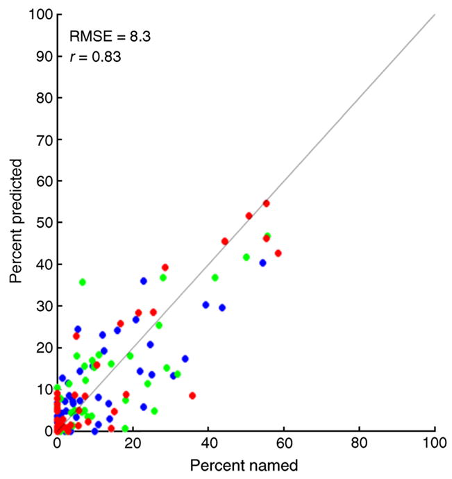
Summary of prediction of color names. Each plotted point shows predicted percent named against measured percent named. Data for all 5 observers and all color names (including white). Blue points: 500-nm spots; green points: 550-nm spots; red points; 600-nm spots.

Discussion

Unpacking the model’s behavior

To help understand what features of the model drive its behavior, we re-modeled the data with a number of model variants. The results of this effort are summarized here and presented and described in more detail in Supplementary Figures S4–S13. Figure S4 replots Figures 6, 10 (right panel), 11, and 12 as a compact montage for reference. Figures S5–S11 provide the same plots for model variants. Figure S12 shows chromaticities of reconstructed flashes when the color or spatial correlations were set to zero in the prior. Figure S13 shows the RMSE error obtained for each model variant.

The conclusions we drew from this exercise are as follows: Run-to-run variability in the overall quality of fit is small (Figure S5), as are the effects of receptor noise in the simulation (Figure S7). In addition, shuffling the locations of the L and M cones in each observer’s mosaic has little effect on the model’s performance, as long as the Bayesian model is constructed with the same mosaic used in the simulations (Figure S6). On the other hand, randomizing the identities of the L and M cones for each observer so that all observer’s mosaics have a common L:M ratio destroys the model’s ability to account for the individual variation in percentage of stimuli named white (Figure S8). Removing individual differences in the optics also reduces the quality of the model fit as measured by overall RMSE, but in this case the pattern of the predictions remains qualitatively consistent with the data (Figure S9). Figures S10–S12 show that incorporating some degree of color and spatial correlation into the priors is crucial to the model’s ability to account for the data.

Model behavior for other stimuli

The model does a reasonable job of predicting the appearance of small-spot colors. More generally, the Bayesian algorithm can reconstruct an image from any set of cone responses, and we thought it important to explore the behavior of this algorithm for stimuli closer to everyday experience than small monochromatic spots viewed under adaptive optics conditions. We investigated the model’s behavior for larger monochromatic spots at suprathreshold intensities and for sinusoidal modulations along three color directions.

Larger suprathreshold spots

Figure 13 shows the reconstructed chromaticities of 550-nm suprathreshold 8-arcmin spots. Three features of the reconstructions are apparent when compared with the corresponding reconstructions for small spots (compare with Figure 9): The variability is greatly reduced within observer, the variability is greatly reduced between observers, and the reconstructed chromaticities are much closer to that of the 550-nm stimulus. These same features hold for the other observers and wavelengths, as illustrated by the naming histograms shown in Figure 14. The naming is consistent across observers. The names for the 500- and 550-nm spots correspond to what we expect from standard accounts of the appearance of monochromatic lights (e.g., Hunt, 1987, p. 130). Spots of 600 nm are generally named orange rather than the predicted yellow. As we note in the caption for Supplementary Figure S5, the data do not sharply constrain the naming boundary that separates yellow from orange. This is the probably cause of the misprediction for the 600-nm spots.

Figure 13.

Reconstructed chromaticities for 8-arcmin spots. The figure shows the reconstructed chromaticities for flashed 8-arcmin 550-nm suprathreshold monochromatic spots, for two observers. Color naming boundaries shown are those derived from the simulations of the small spot experiments (see Figure 4 above). Simulations were performed as for the small spots, using the adaptive optics point spread functions to compute the retinal images. Left panel: observer AP (LM ratio 1.3:1). Right panel: observer BS (LM ratio 14.7:1).

Figure 14.

Predicted naming for 8-arcmin spots. Each bar plot shows the percent names for all 5 observers and one wavelength for flashed 8-arcmin monochromatic spots. Each plot is in the same format as the bottom panel of Figure 2. Naming boundaries used to compute color names were those derived from the small (0.3 arcmin) spot simulations. Simulation details as described in the caption of Figure 13 above. Plots from top to bottom, wavelengths are 500, 550, and 600 nm, respectively. Within each plot, observers are ordered from left to right HS, YY, AP, MD, and BS.

Suprathreshold gratings

Sinusoidal modulations have been employed extensively as stimuli to probe visual processing of spatial and chromatic information (e.g., Campbell & Robson, 1968; de Lange, 1958; Mullen, 1985; Sekiguchi, Williams, & Brainard, 1993). We applied the Bayesian reconstruction algorithm to such gratings. We simulated isochromatic gratings, red/green isoluminant gratings that modulated the L and M cones in counterphase, and gratings that isolated the S cones. Our interest was to verify that the model produced reasonable output for these spatially extended stimuli. Since the model is designed to account for appearance and not thresholds, we ran our simulations at fixed contrasts for each color direction. Figure 15 shows simulated and reconstructed gratings corresponding to 6 cycles per degree (cpd). At this spatial frequency, the isochromatic and red/green gratings are reconstructed veridically. There is a small amount of distortion visible in the S-cone grating reconstruction that arises because of aliasing by the sparse S-cone submosaic (also see below). The reconstructions at lower spatial frequencies, including 0 cpd, appear similarly veridical. Thus, the Bayesian model is consistent with the fact that we see the world with little distortion at low-spatial frequencies.

Figure 15.

Reconstructed low-spatial frequency sinusoidal gratings. The top row shows patches of isochromatic, red/green isoluminant, and S-cone grating modulations that correspond to a spatial frequency of 6 cpd. The middle and bottom rows show, for two observers, the reconstructed stimuli obtained by applying the Bayesian algorithm to the cone responses from these gratings. Simulated grating LMS contrasts were [0.75 0.75 0.75], [0.062, −0.12, 0.00], and [0, 0, 0.66] for the three modulation directions, respectively. These contrasts fit within the gamut of a typical CRT monitor. Mean stimulus chromaticity was that of CIE illuminant D65 (the prior mean), and the mean stimulus intensity was chosen to be ~1.5 log units above the small-spot 50%-seeing threshold intensity. Simulations were performed using the mosaics of observer AP (middle row) and BS (bottom row), and the retinal images were computed using normal optical PSFs (without adaptive optics correction). Images rendered in the sRGB color space (without gamma correction), scaled to a common maximum and with negative image values truncated to zero.

The left column of Figure 16 shows simulated and reconstructed isochromatic gratings corresponding to 24 cpd. Here distortions are visible in the reconstructions. Although the stimulus grating is visible, it is contaminated by red/green noise. This corresponds to the phenomenon of Brewster’s colors, where red/green mottle is apparent against high-contrast high-spatial frequency luminance gratings. We have argued previously that Brewster’s colors arise as a result of trichromatic sampling by the retinal mosaic (Williams et al., 1991). In that report, a simple model of the reconstruction process accounted for the spatial pattern of the red/green mottle but predicted that it should be much more visually salient than it is. That model was based on independent interpolation of the signals from the L-, M-, and S-cone submosaics. The Bayesian reconstruction algorithm, which jointly processes the responses of the entire mosaic, predicts more subtle effects that are in line with the perceptual phenomenon.

Figure 16.

Reconstructed high-spatial frequency sinusoidal gratings. The top row shows patches of isochromatic, red/green isoluminant, and S-cone grating modulations that correspond to a spatial frequencies of 24, 24, and 15 cpd, respectively. The middle and bottom rows show the reconstructed stimuli obtained by applying the Bayesian algorithm to the cone responses from these gratings, for two observers. Other details as with Figure 15 above.

The center column of Figure 16 shows simulated and reconstructed red/green gratings at 24 cpd. The reconstruction distorts the spatial structure of the stimulus grating. Although red/green gratings are typically below detection threshold at 24 cpd when viewed with normal optics (Mullen, 1985), they can be detected when presented using interferometric techniques that bypass optical blurring (Sekiguchi et al., 1993). In this case, the percept at detection threshold is one of spatial noise (Sekiguchi et al., 1993), perhaps consistent with the Bayesian algorithm’s reconstruction.

The right column of Figure 16 shows simulated and reconstructed S-cone gratings at 15 cpd. As the spatial frequency of S-cone gratings increases, distortions referred to as S-cone aliasing occur because of the sparse sampling of the S-cone submosaic (Williams & Collier, 1983). The splotchy nature of the reconstructed patterns reproduce this phenomenon.

Figure 17 summarizes the relation between simulated and reconstructed stimuli for modulations between 0 and 60 cpd for all three color directions investigated. For each stimulus, we computed the projection of the reconstructed image onto the stimulus image, after subtraction of the mean image. We then took the ratio of the contrast power of the stimulus and projected images. This provides a single number measure of how much of the input image makes it through the reconstruction process. We plotted this measure, which we refer to as the projection contrast sensitivity, against spatial frequency for all three color directions. Each function was normalized by its value for 0 cpd.

Figure 17.

Projection contrast sensitivity. The plot shows the projection contrast sensitivity (see description in text) for two observers as a function of grating spatial frequency for isochromatic (black), red/green isoluminant (red), and S-cone isolating gratings (blue). Values shown are the average of values obtained for gratings in sine and cosine spatial phase. Top panel, observer AP; bottom panel, observer BS.

For observer AP (top panel), the plot falls off most rapidly for the S-cone gratings. This effect is due to axial chromatic aberration, which reduces the optical quality for stimuli seen by S cones relative to those seen by M and L cones, and the sparse sampling provided by the S cone submosaic. More interesting is the fact that the red/green function falls off more rapidly than the isochromatic function. This effect is a fundamental consequence of the fact that L and M cone signals are highly correlated in prior distribution used by the Bayesian algorithm. At any spatial frequency, a luminance grating is more likely a priori than a red/green grating. In addition, the high correlation between neighboring pixels in the prior makes low spatial frequency stimuli more likely a priori than high spatial frequency stimuli. As the spatial frequency of the stimulus gratings increases, the reconstructed power falls off in part because of optical blurring. But this blurring affects isochromatic and red/green isoluminant gratings to about the same degree. The differential effect seen in the top panel of the figure occurs because the prior, which favors low frequency interpretations in the face of ambiguity introduced by trichromatic sampling, begins to dominate earlier for red/green gratings than for isochromatic gratings. For observer BS (bottom panel), who has very few M cones, the spatial falloff for red-green gratings is comparable to that of the S-cone isolating gratings. The difference in predicted performance for the two observers suggests that carefully tailored experiments with gratings might be able to reveal individual differences in L:M cone ratio.

Quality of model fit

It is worth emphasizing that the model does not provide a perfect account of the experimental data. It would almost certainly be possible to improve the model fit by adding more parameters. For example, we could have parameterized the chromaticity region corresponding to white with an ellipse rather than a circle, allowed the boundaries between chromatic color names to curve instead of being straight lines (Abney effect), allowed the boundaries to depend on the luminance of the reconstructed spots (Bezold-Brüke hue shift), or modeled some degree of individual differences in color naming boundaries. We could also have accounted for individual differences in spectral sensitivity of L and M cones (see for example the analysis of ERG data in Brainard et al., 2000), explored a wider range of detection models to try to find one that improved the fit to the naming data, or attempted to model effects of post-isomerization noise.

We did not think that any of the above data-fitting exercises would yield much additional insight. Indeed we see the degree of agreement between model and data as quite encouraging, given the relative simplicity of the approach. As the experimental procedures for conducting psychophysics under adaptive optics conditions are refined, it should be possible to determine more precisely the degree to which incorporating additional factors is required. For example, our current analysis does not rule out the possibility that some aspects of color naming boundaries vary systematically with L:M cone ratio, but a data set that intermixed naming of small and large spots would provide a direct test of this possibility.

Predictions

The model in its current form highlights the fundamental consequences of interleaved trichromatic sampling for visual performance. In this regard, a promising future direction is to use the model to motivate experiments that more sharply test its predictions. These concern primarily the way that color naming of small spots should vary within observer, as a function of the mosaic surrounding a single stimulated cone. Here we outline two such predictions. First, how should the fraction of white responses to small monochromatic spots vary, within observer, with the structure of the mosaic in the neighborhood of the test flash. Second, how should the percentage of blue and green responses for flashes detected by M cones vary, again within observer, as a function of the distance to the nearest S cone. Although testing these predictions requires refinement of the experimental procedures to allow recording of the retinal location of the flashed spots on a trial-by-trial basis, we expect that this will soon be feasible. Such experiments may also clarify the conditions that lead to spots that are seen but that are nonetheless described as unnamable by observers and allow us to understand whether this phenomenon depends systematically on properties of the mosaic.

Effect of local mosaic properties one percent named white

Since in our simulations we know the location of every simulated flash, we binned the data over flashes that landed in similar local neighborhoods and computed the percentage of flashes named white as a function of the neighborhood properties. Figure 18 shows the results of this calculation. The x-axis shows the number of L cones among the 10 cones nearest to the location of the flashed spot; the y-axis shows the corresponding predicted percentage of flashes named white. Each individual line in the plot was derived from the data for a different observer and spot wavelength. The individual lines do not span the entire x-axis because there were not enough flashes in every bin to compute a meaningful prediction; we only plotted data for bins that contained more than 10 seen flashes (from simulations of 2000 flashes).

Figure 18.

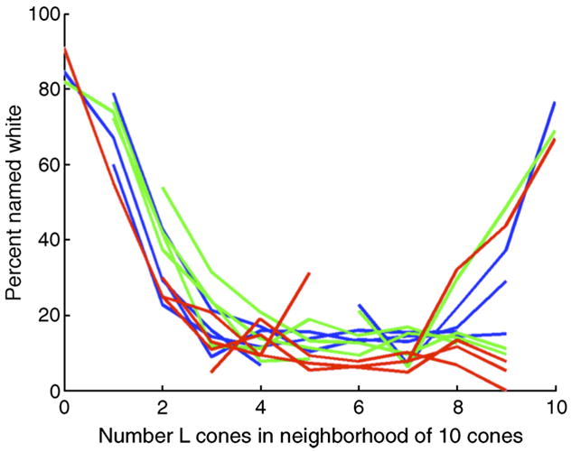
Predicted dependence of percent named white on local mosaic. The figure shows the predicted percentage of spots named white as a function of the local mosaic in the vicinity of the spots. The x-axis is the number of L cones among the 10 cones nearest to the retinal location of the simulated flashed spot. The y-axis is the corresponding percentage of spots named white. Each individual line in the plot shows data derived from simulations of one wavelength and observer. Blue: 500-nm spots; green: 550-nm spots; red; 600-nm spots.

The overall form of the predictions is clear. The number of flashes named white depends strongly on the number of L cones in the local neighborhood and is highest for asymmetric local neighborhoods (i.e., those with mostly L or mostly M cones). The percentage of flashes named white is not highly sensitive to between observer differences or to flash wavelengths, beyond the fact that it may be difficult for some observers and wavelengths to aggregate sufficient data to trace out the entire function.

M cones and blue

In classical color theory, signals from M cones contribute to the sensation of green through a red/green opponent pathway and to the sensation of yellow through a blue/yellow opponent pathway (Hurvich, 1981; Kaiser & Boynton, 1996). There have, however, been suggestions that under some conditions signals from M cones can contribute to the sensation of blue, particularly for small spots (DeValois & DeValois, 1993; Drum, 1989; Schirillo & Reeves, 2001, suggestion attributed to B. Drum by the authors; Hofer, Singer, et al., 2005, suggestion attributed to D. MacLeod by the authors). Here we examine the predictions of the Bayesian model in this regard for the color appearance of small flashes.

Figure 8 above shows that the color of a spot reconstructed from stimulation of an M cone can depend on whether there is an S cone nearby. Figure 19 summarizes this effect for the overall set of simulations that we performed. Seen flashes such that the nearest two cones to the flash location were M cones were selected from all flashes used in the main simulation (5 observers, 3 wavelengths). For each flash, if there was an S cone within the 100 cones nearest to the flash location, the distance to the nearest S cone was computed. Flashes were grouped according to this distance in 1-arcmin bins. For each bin, the percent of all flashes named blue and the percent of all flashes named green were then computed. The plot shows that green responses are more prevalent when an S cone is nearby the flash location and decrease as the distance to the nearest S cone increases, while the opposite relation holds for blue responses. Thus, consistent with some of the earlier suggestions cited above, the Bayesian algorithm predicts that whether an M cone contributes to blueness or greenness varies and depends on whether or not there is an S cone nearby.

Figure 19.

Effect of nearby S cones on appearance of spots seen by M cones. Flashes such that the nearest two cones to the flash location were M cones were selected from all flashes used in the main simulation (5 observers, 3 wavelengths). For each flash, if there was an S cone within the 100 cones nearest to the flash location, the distance to the nearest S cone was computed. Flashes were grouped according to this distance in 1-arcmin bins. For each bin, the percent of all flashes named blue and the percent of all flashes named green were then computed. The plot shows the results (blue line, percent named blue; green line, percent named green). Data from a bin were plotted if the bin represented at least 10 flashes.

Improving the Bayesian algorithm

The present algorithm is based on normal priors and additive normal noise. This choice was based on considerations of analytic and computational convenience. More realistic priors would incorporate a positivity constraint on the reconstructed image and non-normal features of natural images (Simoncelli, 2005). As suggested to us by L. Paninski, it may also be feasible to implement a Poisson rather than additive normal noise model. It will be interesting to see whether and how the reconstruction algorithm’s behavior varies as these more realistic assumptions are added. Our belief is that the basic structural features of the reconstructions will remain unaltered and that the changes will be reflected in reasonably subtle features of the performance and predictions.

Relation to other work on optimal color processing

A number of authors have considered optimal visual processing of color information. This approach has been effective in accounting for spectral properties of cone photoreceptors (e.g., Regan et al., 2001), the approximate receptive field structure of retinal ganglion cells and cortical units (e.g., Atick, Li, & Redlich, 1992; Buchsbaum & Gottschalk, 1983; Caywood, Willmore, & Tolhurst, 2004; Derrico & Buchsbaum, 1990; Doi, Inui, Lee, Wachtler, & Sejnowski, 2003; Lee, Wachtler, & Sejnowski, 2002; Párraga et al., 1998, 2002; Ruderman et al., 1998; van Hateren, 1993; Wachtler, Doi, Lee, & Sejnowski, 2007), the division of information between ON and OFF pathways (von der Twer & MacLeod, 2001; see also Ratliff, 2007), and the shape of ganglion cells’ static non-linearities (von der Twer & MacLeod, 2001). In this paper, we add color appearance phenomena to the exemplars that may be understood as a consequence of optimal processing. Common to our work and the earlier work is the central role played by the statistical structure of natural images. Our work differs from the earlier work in two important ways. First, of the above papers, only a few (Doi et al., 2003; Wachtler et al., 2007) explicitly consider the trichromatic sampling of the cone mosaic, while this is a key feature of our model. Second, rather than optimizing signal-to-noise (or information transmitted), our work emphasizes veridicality of the final perceptual representation.

Interestingly, our model produces a possible functional motivation for the well-known difference between the high-spatial frequency falloff of the isochromatic and chromatic spatial contrast sensitivity functions (Mullen, 1985; Sekiguchi et al., 1993), in that similar behavior is shown by the projection contrast sensitivity functions plotted in Figure 17. In our model, this behavior arises from the properties of the prior distribution and their interaction with information loss from trichromatic sampling when visual processing optimizes veridical representation. To connect our model more fully with threshold data would require elaborations that specify the sources of post-receptoral noise that limit detection and how these interact with trichromatic reconstruction. Such elaborations might also enable principled integration of our model and earlier work that relates to isochromatic and chromatic sensitivity but that emphasizes efficiency of information transmission (Atick et al., 1992; van Hateren, 1993). The approach taken by Abrams, Hillis, and Brainard (2007), who considered the relation between the adaptation required to optimize color discrimination and that required to stabilize color appearance across changes of illumination, could provide guidance in this regard.

Learning cone classes

The Bayesian algorithm incorporates information about the location and class of each cone. Although a discussion of how the visual system might learn this information is well beyond the scope of this paper, Figures S14 and S15 illustrate a possible error signal that could drive a learning algorithm. The idea underlying these figures is due to Maloney and Ahumada (1993), who showed that a visual system could learn the locations of photoreceptors by comparing image reconstructions across eye movements. These should typically be shifted copies of one another since a change in eye position will usually just shift the retinal image and, in the absence of reconstruction error, the reconstructed image will shift by the same amount. This same idea appears to have potential for driving an algorithm that learns cone classes as well. Figure S14 shows pairs of shifted reconstructions based on algorithm that is based on correct knowledge of cone classes, while Figure S15 shows corresponding pairs when the algorithm is based on a partially mistyped mosaic. The errors in the latter case have a characteristic signature that is tied to the mosaic rather than to the input and which we speculate could be used to allow the visual system to learn cone classes. Whether a successful algorithm based on this or other developmental principles (e.g., Dominguez & Jacobs, 2003) can be shown remains an interesting future direction.

Neural implications

The model as we have presented is functional and is based on optimality considerations rather than on known facts about mechanisms in the visual pathways. We noted in the Methods section that the Bayesian reconstruction may be expressed as x_estimate = Iy_noisymosaic + i₀. As emphasized by Brainard et al. (2006), in general the neural implementation of a Bayesian calculation need not resemble its implementation on a digital computer. Here, however, examination of the form of the estimator allows straightforward interpretation of the algorithm in neural terms. If we neglect the i₀ term, we see that the reconstructed image is the weighted sum of a set of basis images, one from each column of the matrix I, with the weight on each column simply being the magnitude of the response of the corresponding cone. We know from examination of these basis images that each represents a blurred colored blob, as in the lower panels of Figures 7 and 8. Thus, we can conceive of a set of neurons, one for each foveal cone, each of which represents a single basis image. A set of second stage neurons could then pool the output of the first to produce a representation of the Bayesian image reconstruction.

A useful insight gained from this perspective is that the Bayesian model can be understood as associating a localized color percept with each individual cone (rather than each individual cone class) and then producing an overall percept that is the sum of the individual cone percepts. This is similar to the elemental sensation assumption made in earlier work that analyzed the appearance of small spot colors (Hartridge, 1954; Krauskopf, 1964, 2000; Krauskopf & Srebro, 1965; Otake, Gowdy, & Cicerone, 2000). This assumption is that a fixed sensation (e.g., red, green, or blue) is associated with stimulation of cones of each class (e.g., L, M, and S). The elemental sensation assumption is difficult to reconcile with the experimental data of Hofer, Singer, et al. (2005), and the current Bayesian model indicates that it is not compatible with optimal reconstruction from the interleaved cone mosaic. The possibility that the elemental sensation assumption does not hold is worth bearing in mind when interpreting conclusions drawn via analyses that incorporate it.

The Bayesian model does suggest a generalization of the elemental sensation assumption, where the percept associated with each cone depends not only on its class but also on the fine structure of the local mosaic in which it is situated. If this more general form of the assumption holds, in which stimulation of any given cone always contributes the same sensation to the overall percept, then we should not expect variability in the color percepts resulting from trials that resulted in the identical array of cone responses. In practice, however, testing this prediction would require accounting for trial-to-trial variability arising from uncontrollable noise sources such as photon noise.

Summary

This paper describes a Bayesian algorithm (Brainard, 1994) for reconstructing full trichromatic images from the responses of interleaved L, M, and S cones. The algorithm is combined with a model of color naming and provides a good account of measurements of the appearance of very small (0.3 arcmin) monochromatic spots presented using adaptive optics (Hofer, Singer, et al., 2005). In particular, the model can account for the fact that small flashed monochromatic spots elicit a wide variety of color names and for the striking individual variation in naming percentages. The latter is driven by corresponding individual variation in the arrangement and relative number of L, M, and S cones in each observer’s mosaic and does not require any free parameters to describe the individual observer differences.

A key emergent feature of the model is that stimulating a single cone of a particular class should yield a different color sensation, depending on the structure of the mosaic surrounding the stimulated cone (see Figures 7 and 8). A particular consequence of this feature is that the percent of flashes named white are predicted to vary systematically with the L:M cone ratio of the mosaic, in a manner consistent with the experimental data.

The model also accounts for other color appearance phenomena. It correctly predicts that within and between observer variation in naming will decrease dramatically for larger (8 arcmin) spots at suprathreshold levels, and it describes distortions of the appearance of fine spatial gratings while at the same time correctly predicting that coarse gratings will be perceived veridically.

Finally, the model makes testable predictions for how the color appearance of very small spots, measured within observer, should depend on the fine structure of the cone mosaic.

References

- Abrams AB, Hillis JM, Brainard DH. The relation between color discrimination and color constancy: When is optimal adaptation task dependent? Neural Computation. 2007;19:2610–2637. doi: 10.1162/neco.2007.19.10.2610. [DOI] [PMC free article] [PubMed] [Google Scholar]
- Atick JJ, Li ZP, Redlich AN. Understanding retinal color coding from 1st principles. Neural Computation. 1992;4:559–572. [Google Scholar]
- Brainard DH. Bayesian method for reconstructing color images from trichromatic samples. Paper presented at the IS&T 47th Annual Meeting; Rochester, NY. 1994. pp. 375–379. [Google Scholar]
- Brainard DH. Colorimetry. In: Bass M, editor. Handbook of optics: Fundamentals, techniques, and design. chap 26. Vol. 1. New York: McGraw-Hill; 1995. pp. 1–54. [Google Scholar]
- Brainard DH, Longère P, Delahunt PB, Freeman WT, Kraft JM, Xiao B. Bayesian model of human color constancy. Journal of Vision. 2006;6(11):10, 1267–1281. doi: 10.1167/6.11.10. http://journalofvision.org/6/11/10/ [DOI] [PMC free article] [PubMed]
- Brainard DH, Roorda A, Yamauchi Y, Calderone JB, Metha A, Neitz M, et al. Functional consequences of the relative numbers of L and M cones. Journal of the Optical Society of America A, Optics, Image Science, and Vision. 2000;17:607–614. doi: 10.1364/josaa.17.000607. [DOI] [PubMed] [Google Scholar]
- Brainard DH, Williams DR. Spatial reconstruction of signals from short-wavelength cones. Vision Research. 1993;33:105–116. doi: 10.1016/0042-6989(93)90063-3. [DOI] [PubMed] [Google Scholar]
- Buchsbaum G, Gottschalk A. Trichromacy, opponent colours coding and optimum colour information transmission in the retina. Proceedings of the Royal Society of London B: Biological Sciences. 1983;220:89–113. doi: 10.1098/rspb.1983.0090. [DOI] [PubMed] [Google Scholar]
- Burton GJ, Moorehead IR. Color and spatial structure in natural images. Applied Optics. 1987;26:157–170. doi: 10.1364/AO.26.000157. [DOI] [PubMed] [Google Scholar]
- Campbell FW, Robson JG. Application of Fourier analysis to the visibility of gratings. The Journal of Physiology. 1968;197:551–566. doi: 10.1113/jphysiol.1968.sp008574. [DOI] [PMC free article] [PubMed] [Google Scholar]
- Caywood MS, Willmore B, Tolhurst DJ. Independent components of color natural scenes resemble V1 neurons in their spatial and color turning. Journal of Neurophysiology. 2004;91:2859–2873. doi: 10.1152/jn.00775.2003. [DOI] [PubMed] [Google Scholar]
- de Lange H. Research into the dynamic nature of the human fovea-cortex systems with intermittent and modulated light. I. Attenuation characteristics with white and coloured light. Journal of the Optical Society of America A. 1958;48:777–784. doi: 10.1364/josa.48.000777. [DOI] [PubMed] [Google Scholar]
- DeMarco P, Pokorny J, Smith VC. Full-spectrum cone sensitivity functions for X-chromosome-linked anomalous trichromats. Journal of the Optical Society of America A, Optics and Image Science. 1992;9:1465–1476. doi: 10.1364/josaa.9.001465. [DOI] [PubMed] [Google Scholar]
- Derrico JB, Buchsbaum G. A computational model of spatiochromatic image coding in early vision. Journal of Visual Communication and Image Representation. 1990;2:31–38. [Google Scholar]
- DeValois RL, DeValois KK. A multistage color model. Vision Research. 1993;33:1053–1065. doi: 10.1016/0042-6989(93)90240-w. [DOI] [PubMed] [Google Scholar]
- Doi E, Inui T, Lee TW, Wachtler T, Sejnowski TJ. Spatiochromatic receptive field properties derived from information-theoretic analyses of cone mosaic responses to natural scenes. Neural Computation. 2003;15:397–417. doi: 10.1162/089976603762552960. [DOI] [PMC free article] [PubMed] [Google Scholar]
- Dominguez M, Jacobs RA. Developmental constraints aid the acquisition of binocular disparity sensitivities. Neural Computation. 2003;15:161–182. doi: 10.1162/089976603321043748. [DOI] [PubMed] [Google Scholar]
- Drum B. Hue signals from short- and middle-wavelength-sensitive cones. Journal of the Optical Society of America A, Optics and Image Science. 1989;6:153–157. doi: 10.1364/josaa.6.000153. [DOI] [PubMed] [Google Scholar]
- Field DJ. Relations between the statistics of natural images and the response properties of cortical cells. Journal of the Optical Society of America A, Optics and Image Science. 1987;4:2379–2394. doi: 10.1364/josaa.4.002379. [DOI] [PubMed] [Google Scholar]
- Gelman A, Carlin JB, Stern HS, Rubin DB. Bayesian data analysis. 2. Boca Raton: Chapman & Hall/CRC; 2004. [Google Scholar]
- Hansen T, Walter S, Gegenfurtner KR. Effects of spatial and temporal context on color categories and color constancy. Journal of Vision. 2007;7(4):2, 1–15. doi: 10.1167/7.4.2. http://journalofvision.org/7/4/2/ [DOI] [PubMed]
- Hartridge H. Color receptors of the human fovea. Nature. 1954;158 doi: 10.1038/158097c0. [DOI] [PubMed] [Google Scholar]
- Hofer H, Carroll J, Neitz J, Neitz M, Williams DR. Organization of the human trichromatic cone mosaic. Journal of Neuroscience. 2005;25:9669–9679. doi: 10.1523/JNEUROSCI.2414-05.2005. [DOI] [PMC free article] [PubMed] [Google Scholar]
- Hofer H, Singer B, Williams DR. Different sensations from cones with the same photopigment. Journal of Vision. 2005;5(5):5, 444–454. doi: 10.1167/5.5.5. http://journalofvision.org/5/5/5/ [DOI] [PubMed]
- Hunt RWG. The reproduction of colour. 4. Tolworth, England: Fountain Press; 1987. [Google Scholar]
- Hurvich LM. Color vision. Sunderland, MA: Sinauer Association; 1981. [Google Scholar]
- Jaaskelainen T, Parkkinen J, Toyooka S. A vector-subspace model for color representation. Journal of the Optical Society of America A. 1990;7:725–730. [Google Scholar]
- Kaiser PK, Boynton RM. Human color vision. 2. Washington, DC: Optical Society of America; 1996. [Google Scholar]
- Kelly KL. Color designations for lights. Journal of the Optical Society of America A. 1943;33:627–632. [Google Scholar]
- Krauskopf J. Color appearance of small stimuli and the spatial distribution of color receptors. Journal of the Optical Society of America A. 1964;54:1171. [Google Scholar]
- Krauskopf J. Relative numbers of long- and middle-wavelength-sensitive cones in the human fovea. Journal of the Optical Society of America A, Optics, Image Science, and Vision. 2000;17:510–516. doi: 10.1364/josaa.17.000510. [DOI] [PubMed] [Google Scholar]
- Krauskopf J, Srebro R. Spectral sensitivity of color mechanisms: Derivation from fluctuations of color appearance near threshold. Science. 1965;150:1477–1479. doi: 10.1126/science.150.3702.1477. [DOI] [PubMed] [Google Scholar]
- Lee TW, Wachtler T, Sejnowski TJ. Color opponency is an efficient representation of spectral properties in natural scenes. Vision Research. 2002;42:2095–2103. doi: 10.1016/s0042-6989(02)00122-0. [DOI] [PMC free article] [PubMed] [Google Scholar]
- Maloney LT. Evaluation of linear models of surface spectral reflectance with small numbers of parameters. Journal of the Optical Society of America A, Optics and Image Science. 1986;3:1673–1683. doi: 10.1364/josaa.3.001673. [DOI] [PubMed] [Google Scholar]
- Mullen KT. The contrast sensitivity of human colour vision to red-green and blue-yellow chromatic gratings. The Journal of Physiology. 1985;359:381–400. doi: 10.1113/jphysiol.1985.sp015591. [DOI] [PMC free article] [PubMed] [Google Scholar]
- Nascimento SM, Ferreira FP, Foster DH. Statistics of spatial cone-excitation ratios in natural scenes. Journal of the Optical Society of America A, Optics, Image Science, and Vision. 2002;19:1484–1490. doi: 10.1364/josaa.19.001484. [DOI] [PMC free article] [PubMed] [Google Scholar]
- Otake S, Gowdy PD, Cicerone CM. The spatial arrangement of L and M cones in the peripheral human retina. Vision Research. 2000;40:677–693. doi: 10.1016/s0042-6989(99)00202-3. [DOI] [PubMed] [Google Scholar]
- Párraga CA, Brelstaff G, Troscianko T, Moorehead IR. Color and luminance information in natural scenes. Journal of the Optical Society of America A, Optics, Image Science, and Vision. 1998;15:563–569. doi: 10.1364/josaa.15.000563. [DOI] [PubMed] [Google Scholar]
- Párraga CA, Troscianko T, Tolhurst DJ. Spatiochromatic properties of natural images and human vision. Current Biology. 2002;12:483–487. doi: 10.1016/s0960-9822(02)00718-2. [DOI] [PubMed] [Google Scholar]
- Pratt WK. Digital image processing. New York: John Wiley & Sons; 1978. [Google Scholar]
- Ratliff CP. Unpublished PhD thesis. Philadelphia: University of Pennsylvania; 2007. Toward a theory of functional organization of the retina. [Google Scholar]
- Regan BC, Julliot C, Simmen B, Viénot F, Charles-Dominique P, Mollon JD. Fruits, foliage and the evolution of primate colour vision. Philosophical Transactions of the Royal Society of London B: Biological Sciences. 2001;356:229–283. doi: 10.1098/rstb.2000.0773. [DOI] [PMC free article] [PubMed] [Google Scholar]
- Roorda A, Williams DR. The arrangement of the three cone classes in the living human eye. Nature. 1999;397:520–522. doi: 10.1038/17383. [DOI] [PubMed] [Google Scholar]
- Ruderman DL, Cronin TW, Chiao CC. Statistics of cone responses to natural images: Implications for visual coding. Journal of the Optical Society of America A. 1998;15:2036–2045. [Google Scholar]
- Schirillo J, Reeves A. Color-naming of M-cone incremental flashes. Color Research and Application. 2001;26:132–140. [Google Scholar]
- Sekiguchi N, Williams DR, Brainard DH. Aberration-free measurements of the visibility of isoluminant gratings. Journal of the Optical Society of America A, Optics, Image Science, and Vision. 1993;10:2105–2117. doi: 10.1364/josaa.10.002105. [DOI] [PubMed] [Google Scholar]
- Simoncelli EP. Statistical modeling of photographic images. In: Bovik A, editor. Handbook of image and video processing. Boston: Academic Press; 2005. pp. 431–441. [Google Scholar]
- Smith VC, Pokorny J. Spectral sensitivity of the foveal cone photopigments between 400 and 500 nm. Vision Research. 1975;15:161–171. doi: 10.1016/0042-6989(75)90203-5. [DOI] [PubMed] [Google Scholar]
- van Hateren JH. Spatial, temporal and spectral pre-processing for colour vision. Proceedings of the Royal Society B: Biological Sciences. 1993;251:61–68. doi: 10.1098/rspb.1993.0009. [DOI] [PubMed] [Google Scholar]
- von der Twer T, MacLeod DI. Optimal nonlinear codes for the perception of natural colors. Network. 2001;12:395–407. [PubMed] [Google Scholar]
- Wachtler T, Doi E, Lee T, Sejnowski TJ. Cone selectivity derived from the responses of the retinal cone mosaic to natural scenes. Journal of Vision. 2007;7(8):6, 1–14. doi: 10.1167/7.8.6. http://journalofvision.org/7/8/6/ [DOI] [PMC free article] [PubMed]
- Wandell BA. Foundations of vision. Sunderland, MA: Sinauer; 1995. [Google Scholar]
- Williams DR, MacLeod DI, Hayhoe MM. Foveal tritanopia. Vision Research. 1981;21:1341–1356. doi: 10.1016/0042-6989(81)90241-8. [DOI] [PubMed] [Google Scholar]
- Williams DR, Collier R. Consequences of spatial sampling by a human photoreceptor mosaic. Science. 1983;221:385–387. doi: 10.1126/science.6867717. [DOI] [PubMed] [Google Scholar]
- Williams DR, Sekiguchi N, Haake W, Brainard DH, Packer O. The cost of trichromacy for spatial vision. In: Lee BB, Valberg A, editors. From pigments to perception. New York: Plenum Press; 1991. pp. 11–22. [Google Scholar]
- Wyszecki G, Stiles WS. Color science: Concepts and methods, quantitative data and formulae. 2. New York: John Wiley & Sons; 1982. [Google Scholar]