A modified hyperplane clustering algorithm allows for efficient and accurate clustering of extremely large datasets

Abstract

Motivation: As the number of publically available microarray experiments increases, the ability to analyze extremely large datasets across multiple experiments becomes critical. There is a requirement to develop algorithms which are fast and can cluster extremely large datasets without affecting the cluster quality. Clustering is an unsupervised exploratory technique applied to microarray data to find similar data structures or expression patterns. Because of the high input/output costs involved and large distance matrices calculated, most of the algomerative clustering algorithms fail on large datasets (30 000 + genes/200 + arrays). In this article, we propose a new two-stage algorithm which partitions the high-dimensional space associated with microarray data using hyperplanes. The first stage is based on the Balanced Iterative Reducing and Clustering using Hierarchies algorithm with the second stage being a conventional k-means clustering technique. This algorithm has been implemented in a software tool (HPCluster) designed to cluster gene expression data. We compared the clustering results using the two-stage hyperplane algorithm with the conventional k-means algorithm from other available programs. Because, the first stage traverses the data in a single scan, the performance and speed increases substantially. The data reduction accomplished in the first stage of the algorithm reduces the memory requirements allowing us to cluster 44 460 genes without failure and significantly decreases the time to complete when compared with popular k-means programs. The software was written in C# (.NET 1.1).

Availability: The program is freely available and can be downloaded from http://www.amdcc.org/bioinformatics/bioinformatics.aspx.

Contact: rmcindoe@mail.mcg.edu

Supplementary information: Supplementary data are available at Bioinformatics online.

1 INTRODUCTION

Clustering gene expression data can be done using either supervised or unsupervised algorithms that group genes with similar expression pattern. For unsupervised methods, the similarity between gene expression vectors is calculated using a distance metric. Common distance metrics used for this purpose are Euclidean, Manhattan and Pearson. The goal of clustering is to minimize the intracluster distances and to maximize the intercluster distances. There are many data clustering algorithms available in the literature with the three most popular clustering algorithms used for clustering gene expression data being: Hierarchical Clustering; k-means; and self organizing maps (SOM). These methods are popular because of their conceptual simplicity and their availability in standard software packages rather than their algorithmic qualities (Handl et al., 2005).

Hierarchical Clustering is widely used in the scientific community because it is easy to read and interpret due to better visualization of clusters using a dendrogram (assuming the dataset size is small). In this method, a pairwise distance matrix is calculated for all the genes prior to the construction of the dendrogram. Initially, all genes are considered as individual clusters followed by sequential merging of the two closest clusters in each subsequent step based on their distance. The final step has only one cluster left with all the genes in it. The dendrogram represents the hierarchy of clusters in the dataset based on their distance from one another. When merging two clusters, one must calculate the new distance for the merged cluster. Three different methods can be used to calculate the new cluster distance; single linkage, average linkage and complete linkage. Single linkage takes the smaller of the two distance values, complete linkage takes the greater of the two distance values and average linkage takes the average of the two distance values.

The k-means and SOM are partition based algorithms and therefore clusters are not represented as hierarchies but rather the genes are grouped into partitions based on their similarity in expression. These two methods have been consistently reported to perform better than other methods, such as hierarchical clustering (Chen et al., 2002; Datta and Datta, 2003; Thalamuthu et al., 2006). As the number of genes on a single microarray chip increases with technological advances, the size of the dataset becomes an issue in cluster analysis. Most of the available algorithms are good for small datasets, but either fail or have difficulty completing when analyzing large datasets (e.g. tens of thousands of genes by hundreds of arrays). Because most of the conventional clustering algorithms require multiple iterative scans of the data and intermediate calculations, a significant amount of memory and CPU time is required to perform cluster analysis for large datasets. For example, using a desktop computer, it is time consuming and difficult to cluster >30 000 genes × 100 arrays using the available algorithms. The memory requirements and computation time increases dramatically as the dataset size increases with the complexity being proportional to the square of the dataset size. To address this issue we have developed a two-stage algorithm designed to cluster large datasets. The first stage of the algorithm reduces the data complexity using the Balanced Iterative Reducing and Clustering using Hierarchies (BIRCH) algorithm (Zhang et al., 1996). This data reduction step is done in a single scan of the data and reduces the memory requirements. The second stage uses the resulting partitions from the first stage and performs a conventional k-means algorithm on the reduced dataset. This algorithm has been implemented in a software application designed to analyze microarray data.

To test this algorithm, we used both simulated and real datasets. The simulated datasets have defined clusters with known results and are used to assess the accuracy of the algorithm. Our results indicate the modified hyperplane algorithm is significantly faster than existing algorithms, using substantially reduced memory requirements and provides comparable accuracy and quality when evaluated relative to existing algorithms.

2 METHODS

2.1 Algorithm

The modified hyperplane clustering algorithm (HPCluster) works in two stages: (i) reduction of the dataset using cluster features (CFs) and (ii) conventional k-means clustering on the CFs obtained in stage 1. The first stage of the algorithm is derived from the BIRCH algorithm proposed by Zhang et al. (1996). BIRCH summarizes a dataset into a set of CFs (subclusters) to reduce the scale of the clustering problem. Dense data points that are extremely close to each other are treated collectively as a single CF and not individually.

2.1.1 CF

A CF is a group of closely related data points and is defined based on three variables (N, LS, SS) that summarize information related to the data points in the CF.

(1)

N = Number of data points in the CF. LS = Linear sum of the N vector data points.

(2)

Where X_i is the d-dimensional data point vector.

SS = Sum of the squares of the N data points.

(3)

The centroid, radius and diameter of a CF can be calculated using these variables and are defined as:

(4)

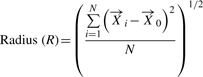(5)

(6)

The first stage of the algorithm is as follows.

1. Calculate the maximum allowable diameter (D_max) for the CFs. D_max is an important parameter which is calculated based on a random sampling of 10% of the genes from the dataset. The details of this step are explained in the next section.

2. The first gene from the dataset becomes the first CF with N = 1.

3. The next gene is added to this first CF.

4. After addition of this gene, the diameter of the CF is calculated. If the diameter is greater than D_max, this gene is taken out and a new CF is made with this gene.

5. The next gene is then compared with each of the CFs and is added to the closest CF.

6. Steps 4 and 5 are repeated till the end of the gene list.

At the end of the first stage, the whole dataset is partitioned into CFs with summary information available for these dense collections of data points. The centroid, radius and diameter of these CFs can be calculated using Equations (4–6). The second stage of the algorithm uses a conventional k-means clustering algorithm. CFs obtained in the first stage are now considered as individual data points and we use the Euclidian distance between two CFs as a measure of the distance between these CFs. The Euclidean distance between two CFs is the distance between their centroids

(7)

The second stage of the algorithm is as follows.

1. Cluster centroids are initialized; the different initialization schemes used are explained in the next section.

2. CFs are assigned to the closest centroids.

3. Cluster centroids are recalculated.

4. Steps 2 and 3 are repeated until there is no change in the centroids.

2.2 Estimation of the maximum diameter of a CF

The degree of data reduction depends upon the maximum allowable size of the CFs, which is a function of the maximum diameter (D_max). A large D_max will result in a smaller number of CFs and hence a greater degree of data reduction whereas a small D_max will result in a larger number of CFs and a lesser degree of data reduction. By setting the D_max, we can control the maximum size (in space) of the CFs. If we over estimate D_max, we will get very few final CFs. If the diameter is too small, than we will get a large number of final CFs. For example, D_max can be set so large that you could result in a single CF containing all the genes in the dataset or so small that the number of CFs is equal to the number of genes. This means we can get 1 − N number partitions of the data depending upon the diameter. Estimating the initial D_max to use in the first stage of the algorithm is an important step.

In order to estimate D_max for the CFs, we use the 90-10 rule suggested by Dash et al. (2003) to assess the similarity of the data between nodes of a cluster. This empirically derived rule is based on the observation that ∼90% of the agglomerations in a hierarchical cluster of non-uniform data will initially have very small distances as compared with the maximum closest pair distances (the last 10% of agglomerations). In order to calculate an appropriate D_max, we perform hierarchical clustering on a random 10% of the genes and create a distance plot of the distance values from the first merge to last merge (iteration number versus closest pair distance). The inflection point of the distance plot indicates a sharp increase from the smallest distance pairs to the largest distance pairs (the last 10% of agglomerations). Below this inflection point the closest pair distances are small (Fig. 1). This inflection point is an appropriate initial value of the maximum diameter because the objective of the first phase is to merge the data points which are extremely close to each other and consider them collectively.

Fig. 1.

Example distance plot using a random 10% of the experimental microarray dataset to calculate the D_max.

2.3 Initial centroid calculation schemes

Because the second phase of the algorithm uses a classic k-means algorithm, the results of the modified hyperplane clustering algorithm are sensitive to the values of the initial centroids used in the second phase. We use two approaches to initialize the centroids.

1. Dense regions from data (DEN): The CF with the maximum number of data points are the dense regions of the dataset. After completing the first stage, we sort the CFs based on the value of N in each CF and use the top k number of clusters as the initial centroids.

2. Random initial assignments (RIA): The initial centroids are calculated based on a random assignment of each gene to a cluster followed by a calculation of the mean for the random clusters. For example, if the algorithm is using k = 3 clusters, the method will randomly assign each gene to one of three clusters. It will then calculate the average for each cluster and use that vector as the initial centroid for each cluster.

2.4 Implementation

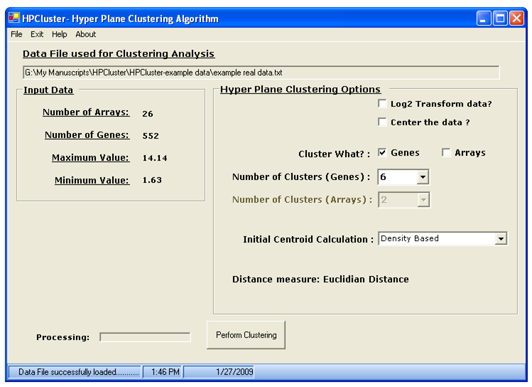
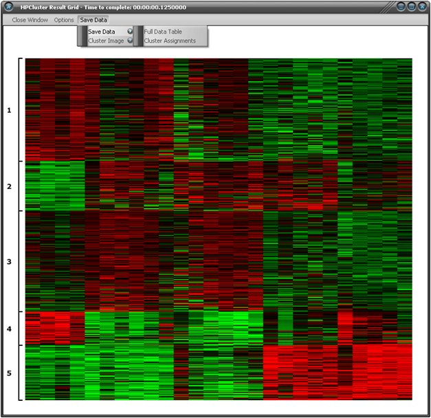
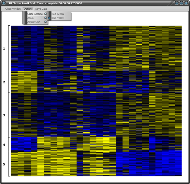
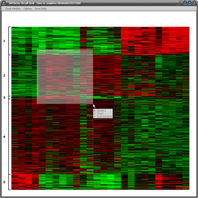
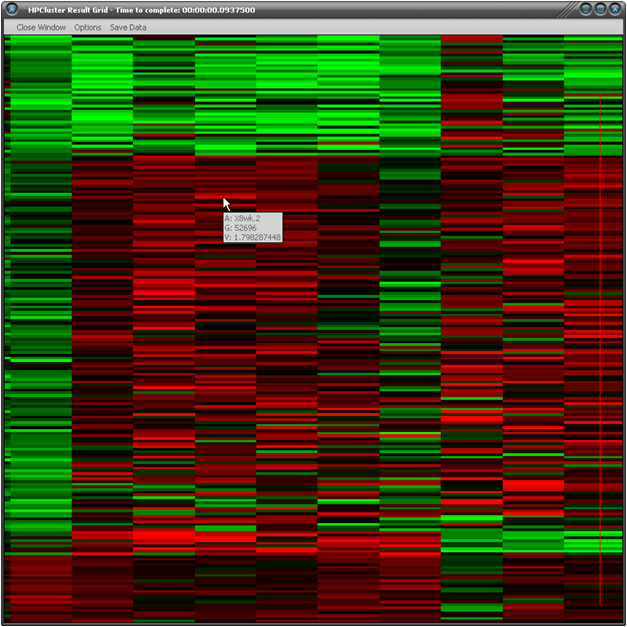
The modified hyperplane clustering algorithm is implemented in a program called HPCluster. This program is a high-performance windows application that implements the two-stage algorithm in a graphical user interface (GUI) application. The program is suited for large datasets because of the decrease in memory usage. All the software was written using the.NET Framework v1.1 and C# as the programming language. Installation of the program is easy and uses the built-in Windows Installer (MSI files). Screen shots of the HPCluster program can be found in the supplemental figures.

2.5 Creation of simulated datasets

We simulated clusters using a cluster-specific pattern across the arrays. In doing so, we created five time points with an equal number of replicates per time point. The mean at the initial time point was chosen randomly from a uniform (−4, 4) distribution. The mean at the subsequent time points was adjusted by a value (β) randomly chosen from a uniform (0, 1) distribution. We introduced ‘cycles’ into the pattern by sampling a new β and changing its sign. The means for the replicates within a time point deviated from the mean for the time point by a value randomly selected from a Gaussian distribution with mean, 0 and variance, 0.1. The number of genes in a cluster was chosen randomly. The mean vector for each gene within a cluster was set by sampling from a Gaussian distribution with mean equal to the cluster mean and variance equal to 0.1. Random noise drawn from a Chi-squared distribution (χ²₆) was added to the resulting matrix of ‘means’. We used a combination of conditions for the number of genes (P = 10 000), number of clusters present (4, 10, 20) and number of arrays (n = 100) in the dataset to generate six total datasets. A heatmap of the simulated 20 cluster dataset is given in the Supplementary Materials (Supplementary Fig. S1).

2.5.1 Experimental microarray data

We also analyzed a real experimentally derived microarray dataset. The dataset was downloaded from the NCBI Gene Expression Omnibus (GEO) (GSE9006: Gene expression in PBMCs from children with diabetes) (Kaizer et al., 2007). The array platform is the Affymetrix GeneChip Human Genome HG-U133A and HG-U133B chips. Combined data from both chips were used for 44 760 genes dataset analyzed. The data from only one chip (HG-U133A) was used for the 22 283 genes dataset and 10 000 randomly picked genes from the HG-U133A set was used for the 10 000 gene dataset.

2.6 Testing the performance of the algorithm

The performance of the algorithm was compared with other popular free clustering algorithms, including GUI based packages. R is a popular open source statistics package that is used extensively by the biomedical community and contains a number of clustering algorithms. For our tests, we used the ‘k-means’ and ‘som’ functions to perform both k-means and SOM clustering using R. We also compared our algorithm with both versions of Cluster (versions 2.0 and 3.0) (Eisen et al., 1998). This Windows based software is used by many biomedical researchers due to the ease of analysis and GUI. All the algorithms were run on a Dell Poweredge 2650 machine with Dual 3.06 GHz/512K Cache Xeon Processors and 8.0 GB DDR 266 MHz RAM.

A common technique used to do meaningful comparisons of gene expression patterns across conditions is to rescale the data by centering the data. This allows one to look for clusters of genes with relatively similar expression patterns across the dataset without concern for the differences in the magnitude of the expression. We standardized the data for each gene separately to center the data,

(8)

where g_ij is the expression value of the i-th gene across the j-th array, is the mean expression of the i-th gene and SD_i is the standard deviation of the i-th gene.

Clustering was performed 12 times on each of the simulated and real microarray datasets for both centered and uncentered data. Three parameters were compared during the testing: time taken, accuracy and stability. Accuracy reflects the similarity between clustering results and the true underlying partitions in the simulated datasets. Stability reflects the similarity between different runs using the same program.

The similarity measure used to compare clustering results was the adjusted Rand index (ARI), which measures the fraction of agreement between two clustering results and can be between 0 and 1, where 1 is perfect agreement (Hubert and Arabie, 1985; Rand, 1971).

3 RESULTS

3.1 Significantly reduced time to completion

In order to assess the speed of the new algorithm, we clustered both the simulated and real microarray datasets for both centered and un-centered data and recorded the time to completion. Each dataset had 100 arrays, varying numbers of genes (10 000, 22 283 and 44 760), varying numbers of clusters (4, 10 and 20) and run 12 times each. The times and cluster assignments were recorded for each run. Table 1 presents the results of this analysis for both the simulated and real microarray centered datasets. All data are the average time in minutes to complete the cluster analysis. We ran our algorithm using the two different centroid initialization schemes (HPC-DEN, HPC-RIA). For comparison, we also ran the same analysis using four clustering algorithms in three software packages. For the HPCluster (HPC) program, the times include the calculation of D_max. All data is the time to complete the algorithm and does not include the time to load the datasets. As can be seen in Table 1, the modified hyperplane clustering algorithm is significantly faster than the R function (k-means) and both versions of Eisen's Cluster program. The improvement in speed is most notable as the datasets analyzed increase in both size and complexity. For example, the time to complete the smallest dataset (10 000 gene real microarray data) with k = 4 clusters shows a significant difference between the two versions of Cluster (5X faster than v2 and 12X faster than v3), but no difference between the R functions. Clustering the same data with k = 20 clusters (more complex) resulted in HPC being significantly faster than the R k-means (4X) and both Cluster versions (18X v2, 29X v3). The largest and most complex dataset analyzed (44 760 genes, k = 20) clearly demonstrated that HPC was significantly faster than all but the R-SOM algorithm (7X R-KM, 35X Cluster v2, 48X Cluster v3). Interestingly, analysis of the time to completion for the un-centered data showed the same significant increase in speed (see Supplementary Table S1) with the exception that the modified hyperplane clustering algorithm performed significantly faster than all the algorithms tested, including R-SOM (26X R-KM, 2X R-SOM, 42X Cluster v2, 112X Cluster v3).

Table 1.

Comparison of time to complete analysis of various clustering algorithms using the centered data

	Simulated dataset			Experimental dataset
Genes	10 000			10 000			22 283			44 760
Clusters	4	10	20	4	10	20	4	10	20	4	10	20
HPC-DEN	0.39±0.04	0.42±0.03	0.46±0.03	0.32±0.01	0.36±0.02	0.67±0.08	0.49±0.07	0.84±0.07	1.48±0.14	1.01±0.17	2.16±0.25	3.37±0.74
HPC-RIA	0.40±0.05	0.62±0.06	0.92±0.09	0.33±0.02	0.41±0.02	0.71±0.09	0.58±0.10	0.92±0.13	1.58±0.15	1.27±0.14	2.41±0.30	4.22±0.44
R-KM	0.23±0.02	0.56±0.07	1.61±0.09	0.24±0.02	0.86±0.08	2.94±0.10	0.59±0.04	2.00±0.09	9.02±0.49	1.07±0.07	4.72±0.19	22.68±1.39
R-SOM	0.22±0.01	0.48±0.04	0.80±0.01	0.21±0.01	0.43±0.01	0.83±0.01	0.44±0.01	0.93±0.03	1.68±0.03	1.01±0.02	1.94±0.04	3.48±0.02
Cluster v2	0.35±0.02	0.62±0.12	1.95±0.45	1.48±0.08	5.09±0.49	11.80±1.20	4.72±0.61	25.94±1.32	45.25±8.81	9.02±2.09	47.75±9.67	118.33±6.51
Cluster v3	1.12±0.08	3.06±0.18	8.94±0.50	3.70±0.42	9.68±0.54	19.28±1.61	8.73±0.28	26.90±1.88	57.50±4.95	11.70±0.56	51.50±2.89	162.33±10.60

HPC-DEN, density from data; HPC-RIA, random initial assignment; R-KM, R-k-mean; R-SOM, R self organizing maps; Cluster v2, Cluster v3, k-means algorithm.

All values for the programs are the average time to completion in minutes and the standard deviation.

N = 12 for each. Bold items indicate significantly lower times within each column.

3.1.1 Scalability of HPC

As the size and complexity of the datasets grow, the scalability of the algorithm becomes more important. An ideal algorithm is one that scales well as the size and complexity of the dataset increases. We used a factorial analysis of variance of time to completion to compare the HPC algorithm to the other clustering algorithms, using the number of clusters, the number of genes and algorithm as the three factors. We then used contrasts to compare algorithms for the linear slopes of the time to completion versus number of genes, separately for each number of clusters. Differences in slope indicate differences in scalability. Since the slopes of all algorithms were compared pairwise, we adjusted our tests using Tukey's HSD. The results of this analysis indicate that the HPC algorithm performs significantly better as the datasets increases in size and complexity. For example, when one uses k = 20 clusters, HPC performs significantly better than all the programs tested (adjusted P < 0.01). However, when k = 10, HPC performs significantly better than all but the R-SOM program (all other programs P < 0.0001, R-SOM P = 0.16).

3.2 Evaluation of cluster quality

In order to evaluate the quality of the cluster assignments produced by the modified hyperplane clustering algorithm, we need to use a statistic that provides a measure of agreement between the cluster results. A common statistic used to evaluate gene clustering methods is the Rand index (Rand, 1971). This statistic indicates the fraction of agreement between two cluster partitions. Agreement can be either pairs of objects that are in the same group in both partitions or in different groups in both partitions. The Rand index can be between 0 and 1 with 1 indicating perfect agreement. The ARI (Hubert and Arabie, 1985; Rand, 1971) adjusts the score so that the expected value in the case of random partitions is 0. The ARI is a popular statistic used to evaluate gene expression clustering algorithms (Kraj et al., 2008; Thalamuthu et al., 2006; Yeung et al., 2003).

We used the ARI to evaluate both the accuracy and stability of the cluster partitions generated by gene clustering methods. Accuracy was evaluated on the simulated datasets using the ARI calculated between the output cluster partitions and the true partitions. Accuracy is difficult to measure with experimentally derived data since the true clusters are not known. However, the true clusters are known for the simulated dataset. Figure 2 presents the average ARI results for the accuracy of the gene assignments for 10 000 genes and 20 true clusters for both the centered and uncentered data after running each program 12 times. The HPC program was run using the two different initialization schemes to determine their effect on cluster accuracy.

Fig. 2.

Accuracy of clustering algorithms using the simulated dataset. Cluster assignments for each algorithm were recorded 12 times each using both centered and uncentered data. The average ARI was calculated for each algorithm.

Interestingly, all the programs tested were sensitive to whether or not the data were centered before clustering. In general, the programs tended to do a better job of clustering the centered data. The exceptions to this are the HPC-RIA and Eisen's Cluster v2, both of which use the same centroid initialization scheme (RIA). With respect to the uncentered data, HPC-RIA was significantly more accurate (ARI = 0.75 ± 0.01) than the other programs tested (P<0.01). However, the R-SOM algorithm had the lowest accuracy (ARI = 0.54) when compared with the other algorithms (average 14% lower). Interestingly, using the density based initialization scheme for the HPC program resulted in an accuracy that was not significantly different than the R-KM function and Cluster v2, but was significantly worse than the RIA initialization scheme.

As stated previously, using the centered data produced different results from all the programs when compared with the uncentered data (Fig. 2). The HPC algorithm using the DEN initialization scheme did significantly better then all programs with an average ARI = 0.89 ± 0.01. In fact, the HPC-DEN analysis averaged 19.3% better accuracy then all the programs. Unlike the previous analysis with uncentered data, the HPC-RIA had the lowest accuracy (ARI = 0.48 ± 0.02) followed by Eisen's Cluster v2 (ARI = 0.55 ± 0.03).

Since accuracy of experimental data is difficult to determine, we examined cluster stability for analyses involving the experimental data. These analyses provide information on the extent to which similar results would be obtained when running the software multiple times. Figure 3 presents the stability plots for both the centered and uncentered 22 283 gene experimental dataset using k = 10 clusters. Similar to the accuracy data, centering the data has an effect on the stability of the HPC algorithm, namely HPC-DEN is more stable for centered data while the HPC-RIA is more stable for the uncentered data. The R-SOM (ARI = 1.0) and Cluster v3 (ARI = 0.98-1.0) algorithms were the most stable followed by the R-KM (ARI = 0.87-0.95), HPC (ARI = 0.64-0.83) and Cluster v2 (ARI = 0.65-0.9).

Fig. 3.

Stability of the clustering algorithms using experimental data (22 283 genes) and searching for 10 clusters. Cluster assignments for each algorithm were recorded 12 times each. The average ARI was calculated for each pairwise comparison for the 12 results from each algorithm. The median for each algorithm is shown as a horizontal bar. C = centered data, U = uncentered data.

Given the level of agreement observed for both the simulated and experimental data, and the accuracy observed for the simulated data, the DEN initialization would be expected to produce a solution that is more accurate than the other methods when the data is centered. On the other hand, the RIA initialization scheme produces cluster partitions that are more accurate when the data is uncentered.

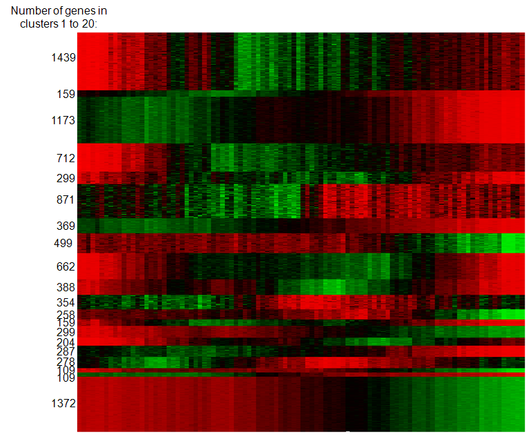
3.3 Effect of incorrect cluster number

The partitioning methods for clustering require that the user provide the number of clusters (k) before executing the algorithm. Determining the appropriate number of clusters to use can be difficult and has an impact on the accuracy and usefulness of the resulting cluster analysis. In order to determine the effect of using an incorrect number of clusters, we ran the modified hyperplane clustering algorithm under varying numbers of clusters. Because we want to assess the accuracy, we used both the centered and uncentered simulated four cluster dataset with 1000 genes and 100 arrays and determined the ARI for the resulting partitions with the programs set to run at 2, 4, 10 and 20 clusters. For comparison, we performed the same cluster analysis using the R functions (k-means and SOM) and Eisen's Cluster v2 and Cluster v3. Figure 4 presents the accuracy plots for each of the programs with the centered data. As expected, each of the programs had their peak ARI value at the correct four cluster analysis with R-SOM (ARI = 0.83) and Cluster v2 (ARI = 0.84) having the lowest values. Once k clusters increase above 4 (the correct number of clusters), the calculated ARIs for the R algorithms (k-means and SOM) and Cluster v3 decrease very quickly (lowest ARI = 0.21). However, the HPC algorithm sustains high accuracy over the entire range of k clusters assessed. For example, the ARI for HPC-DEN at four clusters is 1.0 while the ARI at 20 clusters is 0.97.

Fig. 4.

Accuracy of the clustering algorithms over a range of cluster sizes. The four cluster 1000 gene 100 array centered simulated dataset was analyzed by each program using varying numbers of clusters with the resulting ARI for each analysis plotted.

The uncentered data provided similar results to both the accuracy and stability analyses described in Section 3.2. Specifically, the HPC-RIA initialization scheme performed consistently better across the entire range of k clusters evaluated with the ARI = 0.97-1.0 (4–20 clusters). Interestingly, all other programs, including the HPC-DEN initialization scheme, decreased very quickly as the cluster number increased (Supplementary Fig. S2).

4 DISCUSSION

Clustering of large datasets can be very difficult with the available clustering algorithms mainly due to the memory and time complexity. Hierarchical clustering is suitable for smaller datasets but fails when the datasets become large due to memory constraints of creating the large distance matrices required to perform the clustering algorithm. Additionally, graphical visualization of the larger datasets using a dendrogram is extremely difficult at the lower end of the tree. Therefore, partitioning methods such as k-means or SOM are more suitable to cluster the larger datasets.

The modified hyperplane clustering algorithm described provides a fast and accurate way to cluster very large datasets. Many factors can affect the speed and accuracy of clustering methods. These include not only the size and complexity of the data being analyzed but how it is processed before the partitioning schemes are applied. In this study, we investigated the effect of the number of genes, clusters and arrays on the time to completion as well as the effect of preprocessing the data for our modified hyperplane clustering algorithm.

Depending on the design of the microarray experiment, it may be advantageous to center your data before beginning a cluster analysis. For example, one may want to center the data if the data represents a time course experiment and the investigator is looking for similar expression profile patterns over time without regard to the magnitude of the change. However, if the microarray data represents multiple groups (e.g. four different types of cancer) you may be more interested in absolute expression differences between the groups. Surprisingly, all the programs we tested were sensitive to whether or not the data was centered prior to cluster analysis. The HPC algorithm had the highest accuracy in both the centered (ARI = 0.89 ± 0.01) and un-centered (ARI = 0.75 ± 0.01) datasets. However, the stability of the algorithm was modest when compared with the other programs tested. With respect to the cluster initialization schemes, the DEN based initialization was more accurate when analyzing centered data while the RIA was more accurate for the uncentered data (Fig. 1). Interestingly, one of the most stable programs (R-SOM, ARI = 1.0) had the worst accuracy when the data was centered (ARI = 0.54), indicating that being more stable does not necessarily give you a better answer. In addition, the HPC algorithm preformed consistently better over a wide range of k clusters. Meaning, the cluster solution determined by the HPC program will be robust even if the investigator uses a k that is very different then the true cluster number (Fig. 4).

The advantage of the HPC algorithm is not only can it produce accurate results, but it performs the analysis in a scalable and fast manner. When the datasets are small and less complex (e.g. 10 000 genes, k = 4) all the algorithms tend to run quickly. However, as the datasets increase in size and complexity (e.g. 44 760, k = 20), the HPC algorithm performs significantly faster. Similar to the accuracy data presented, we also observed that centering the data before analysis affected how fast the algorithms completed (Table 1 and Supplementary Table S1). Specifically, the R-KM, R-SOM, Cluster v2 and Cluster v3 all performed significantly slower on the uncentered data. However, the HPC algorithm was not affected and the time to completion was similar for both datasets, especially for the large complex data.

The speed of clustering algorithms will continue to gain in importance. The GEO at NCBI currently has 706 Homo sapiens datasets and over 200 000 gene expression measurements. As the number of publically available microarray experiments increases, the ability to analyze extremely large datasets across multiple experiments becomes critical (Butte and Kohane, 2006). There is a requirement to develop algorithms which are fast and can cluster extremely large datasets without affecting the cluster quality. Here, we present a modified hyperplane clustering two-phase algorithm that solves this problem. To encourage use of this algorithm, we also developed an application (HPCluster) that implements this algorithm and has practical applicability in the scientific community. Screen captures of the program are provided in the Supplementary Material.

Funding: National Institute of Diabetes Digestive and Kidney Diseases (DK076169 to R.A.M.).

Conflict of Interest: none declared.

REFERENCES

- Butte AJ, Kohane IS. Creation and implications of a phenome-genome network. Nat. Biotechnol. 2006;24:55–62. doi: 10.1038/nbt1150. [DOI] [PMC free article] [PubMed] [Google Scholar]
- Chen G, et al. Evaluation and comparison of clustering algorithms in anglyzing ES cell gene expression data. Stat. Sin. 2002;12:241–262. [Google Scholar]
- Dash M, et al. Fast hierarchical clustering and its validation. Data Knowl. Eng. 2003;44:109–138. [Google Scholar]
- Datta S, Datta S. Comparisons and validation of statistical clustering techniques for microarray gene expression data. Bioinformatics. 2003;19:459–466. doi: 10.1093/bioinformatics/btg025. [DOI] [PubMed] [Google Scholar]
- Eisen MB, et al. Cluster analysis and display of genome-wide expression patterns. Proc. Natl Acad. Sci. USA. 1998;95:14863–14868. doi: 10.1073/pnas.95.25.14863. [DOI] [PMC free article] [PubMed] [Google Scholar]
- Handl J, et al. Computational cluster validation in post-genomic data analysis. Bioinformatics. 2005;21:3201–3212. doi: 10.1093/bioinformatics/bti517. [DOI] [PubMed] [Google Scholar]
- Hubert L, Arabie P. Comparing partitions. J. Classif. 1985;2:193–218. [Google Scholar]
- Kaizer EC, et al. Gene expression in peripheral blood mononuclear cells from children with diabetes. J. Clin. Endocrinol. Metab. 2007;92:3705–3711. doi: 10.1210/jc.2007-0979. [DOI] [PubMed] [Google Scholar]
- Kraj P, et al. ParaKMeans: implementation of a parallelized K-means algorithm suitable for general laboratory use. BMC Bioinformatics. 2008;9:200. doi: 10.1186/1471-2105-9-200. [DOI] [PMC free article] [PubMed] [Google Scholar]
- Rand WM. Objective criteria for the evaluation of clustering methods. J. Am. Stat. Assoc. 1971;66:846–850. [Google Scholar]
- Thalamuthu A, et al. Evaluation and comparison of gene clustering methods in microarray analysis. Bioinformatics. 2006;22:2405–2412. doi: 10.1093/bioinformatics/btl406. [DOI] [PubMed] [Google Scholar]
- Yeung KY, et al. Clustering gene-expression data with repeated measurements. Genome Biol. 2003;4:R34. doi: 10.1186/gb-2003-4-5-r34. [DOI] [PMC free article] [PubMed] [Google Scholar]
- Zhang T, et al. BIRCH: an efficient data clustering method for very large databases. ACM SIGMOD Record. 1996;25:103–114. [Google Scholar]
Associated Data
This section collects any data citations, data availability statements, or supplementary materials included in this article.