

Abstract
The continuous measurement of intracranial pressure (ICP) is an important and established clinical tool that is used in the management of many neurosurgical disorders such as traumatic brain injury. Only mean ICP information is used currently in the prevailing clinical practice ignoring the useful information in ICP pulse waveform that can be continuously acquired and is potentially useful for forecasting intracranial and cerebrovascular pathophysiological changes. The present work introduces and validates an algorithm of performing automated analysis of continuous ICP pulse waveform. This algorithm is capable of enhancing ICP signal quality, recognizing non-artifactual ICP pulses, and optimally designating the three well established sub-components in an ICP pulse. Validation of the proposed algorithm is done by comparing non-artifactual pulse recognition and peak designation results from a human observer with those from automated analysis based on a large signal database built from 700 hours of recordings from 66 neurosurgical patients. An accuracy of 97.84% is achieved in recognizing non-artifactual ICP pulses. An accuracy of 90.17%, 87.56%, and 86.53% were obtained for designating each of the three established ICP sub-peaks. These results show that the proposed algorithm can be reliably applied to process continuous ICP recordings from real clinical environment to extract useful morphological features of ICP pulses.
Keywords: Intracranial pressure, traumatic brain injury, hydrocephalus, pulse morphology
I. Introduction
Intracranial pressure measurement is a well established brain monitoring modality used in diagnosing and managing neurosurgical patients in both acute states such as brain injury, severe subarachnoid hemorrhage, and intracerebral hemorrhage and in chronic states such as hydrocephalus. Despite this importance, signal processing capabilities in existing commercial ICP monitoring devices remain poor providing clinicians with limited amount of information that is confined to mean ICP. As a consequence, clinical decisions related to treating ICP related abnormalities are typically made solely based on mean ICP although raw continuous waveform data are usually available. The utilization of only mean ICP, however, ignores the potentially rich information embedded in dynamics of ICP that may be related to cerebral volume compensatory mechanism and cerebral vascular pathophysiology as indicated by some recent methodological advances in ICP analysis [1]–[7].
One very desirable way of characterizing ICP dynamics is through the extraction of morphological features of ICP pulse. It has long-been recognized that pulsatile ICP originates mostly from cerebral arterial pulsations with some contributions of venous origin [8]–[10] and that an ICP pulse is typically triphasic [9] with three sub-peaks. It is thus an advantage to capture alternations in the configuration of these sub-peaks because analysis results would be appealing to clinicians in this familiar way of representing ICP pulse morphology. Furthermore, the alternations of these sub-peak configurations were potentially relevant indicators of decreased intracranial volume compensation [11], [12], intracranial hypertension [13], [14], impaired cerebral blood flow autoregulation [15], and changes in the cerebral vasculature [16], [17]. Despite these previous efforts, the clinical usefulness of analyzing ICP morphology has not yet been unequivocally established [18]. One key technical reason is that most of the studies were conducted in 70s and 80s when the paper charting of ICP waveform was the mainstream practice. As a consequence, only a few ICP morphological features, most of which concerned the overall amplitude or the ratio of the second peak to the first peak, have been studied using either manual or ad hoc extraction methods. Therefore, there is a clear need for automated and robust systems capable of systematically extracting the morphological features of ICP pulse in real time to provide not only amplitude-related features but also features composed of the time intervals of sub-peaks. An overview of the tasks involved in realizing such a system is provided in the following paragraph.
Morphological analysis of ICP pulse involves detection and designation of ICP sub-peaks, which can be decomposed into three sub-tasks. The first task relates to achieving a robust delineation and recognition of each individual ICP pulse. Some solutions [19] of this problem exist but they only partially solve the problem of pulse delineation and are incapable of determining whether an ICP pulse is a non-artifactual one. The second task is to detect all the peaks in each non-artifactual ICP pulse. This is challenging because robust detection of ICP peaks demands a high-quality ICP that cannot always be guaranteed in an ICP recording obtained in an active clinical environment. The third task relates to the designation of the three well-recognized peaks among the detected ICP peak candidates. The solution to this problem is not straightforward because the number of detected ICP peaks could be either greater or smaller than three. It thus challenges an algorithm in correctly (or optimally) allocating the detected peaks when ambiguity exists.
Based on the above analysis, we propose an algorithm that collectively accomplishes the above tasks. The input to the algorithm includes continuous ICP and Electrocardiogram (ECG). The output from the algorithm includes the sequence of locations of three well-recognized ICP peaks (if they exist) of non-artifactual ICP pulses. This algorithm utilizes and integrates several biomedical signal processing and data analysis techniques including ECG QRS detection [20], hierarchical clustering, and an optimal peak designation algorithm. This algorithm is termed Morphological clustering and analysisof ICP pulse (MOCAIP).
The objectives of the present work are to introduce the MOCAIP algorithm and to present an extensive validation of the algorithm. We will discuss the details of the algorithm and the design of the validation procedure in Methods. Validation results are presented and discussed in Results and Discussion, respectively.
II. Methods
A. An introduction of the algorithm
The block diagram of the MOCAIP algorithm is illustrated in Fig. 1. It contains five major components including a beat-by-beat pulse detection component, a pulse clustering component, a non-artifactual pulse recognition component, a peak detection component, and an optimal peak designation component. In addition, the algorithm makes use of a library of reference ICP pulses that contains a collection of pulses and locations of their designated three peaks. The construction of this library of reference pulses can be considered as a training process.
Fig. 1.
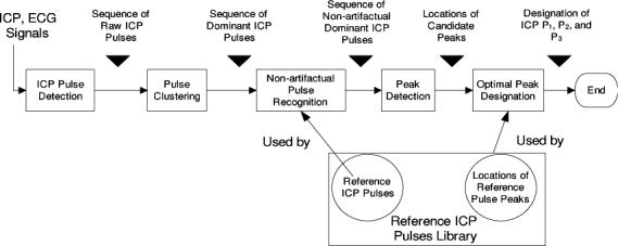
Flow chart of the proposed morphological clustering and analysis of the intracranial pressure. There are five blocks in the flow chart representing the five major processing blocks. In addition, a reference library of non-artifactual ICP pulses and their component peaks is used by the pulse recognition and optimal peak designation blocks of the algorithm.
Beat-by-beat detection of ICP pulse is conducted using an algorithm developed in our previous work [21]. Pulse clustering is used at two stages of processing. It is initially applied to consecutive subsequences of the raw ICP pulses resulted from the ICP pulse detection process to generate a dominant pulse for each sub-sequence. This process results in a sequence of dominant ICP pulses that is further analyzed by the pulse recognition component. Pulse clustering is applied again to the sequence of dominant pulses in this process. The recognized non-artifactual pulses are further processed to detect all peak candidates in each of them. Finally, the peak designation process is executed to optimally designate the three well established ICP peaks in each non-artifactual dominant pulse using the detected peak candidates.
B. ICP pulse detection
We adopted a previously developed method for detecting each ICP pulse [21]. Instead of solely using ICP for pulse detection, we used the mature technique of ECG QRS detection to first find each ECG beat [20]. Besides leveraging the mature ECG QRS detection to achieve reliable ICP pulse detection, we incorporated interval constraints for ICP peak locations to prevent false ICP pulse detections that would be caused by spurious ECG QRS detections. These intervals were also adapted on a beat-by-beat basis. The details of the algorithm and its validation results can be found in [21].
C. Pulse clustering
ICP recordings can be contaminated by several types of noise and artifacts. This is illustrated in Fig. 2 with some representative examples we encountered in practice. Panel A of the figure shows an ICP contaminated by high frequency noise that originated from measurement or amplifier devices. Panel B shows an ICP recording with transient artifacts from coughing or patient movement. Panel C shows an ICP recording with ICP sensor actually detached from the patient monitor from 10th minute to 30th minute. Finally, panel D shows an ICP with a low quantization level, which is usually the case for data collected from the GE Solar 8000 or Dash 4000 bedside monitors that are currently used in our center. These artifacts and noise are not uncommon for typical ICP recordings. Poor quality of recorded individual ICP pulses severely hampers the feasibility of conducting the intended analysis of morphological changes of ICP pulses. We therefore reason that a sensible tradeoff can be made to conduct the analysis of ICP pulse morphology by not using individual pulse but rather using a representative cleaner pulse to be extracted from a sequence of consecutive raw ICP pulses. Hence, a continuous ICP recording can be segmented into consecutive sequences, morphological characteristics of which can be calculated based on the representative pulse of each sequence.
Fig. 2.

Four representative examples of influence of noise and artifacts on ICP recordings. Panel A displays an example of ICP pulse contaminated by high frequency noise; Panel B shows an example of artifacts of transient nature such as coughing; Panel C shows a long recording (50 minutes) that contains a period with ICP sensor actually detached from the monitor in which case an artifactual dominant pulse can still be obtained; Panel D represents an ICP recording with a low quantization level. Poor quality of pulsatile ICP signals, as represented in these examples, would severely hamper the feasibility of extracting morphological features from individual ICP pulse. This motivated us to adopt a pulse clustering technique as discussed in Section II-C.
1) Hierarchial clustering
We propose to use a clustering method to extract a representative ICP pulse from each sequence in the following way. A sequence of raw ICP pulse is first clustered into distinct groups based on their morphological distance. The largest cluster will then be identified. An averaging process will be conducted to obtain an averaged pulse for this largest cluster. In this paper, we call this average pulse of the largest cluster the dominant ICP pulse. This dominant pulse has several desirable properties for performing morphological analysis. First, the clustering procedure will effectively isolate transient disturbance from normal ICP pulses. Therefore, the dominant ICP pulse would most likely represent the signal group. Second, the averaging process effectively reduces influences from random noise and quantization noise on morphological analysis of ICP pulse by enhancing the signal to noise ratio. This averaging technique has been routinely used in extracting high-fidelity signals from repeatedly measured evoked potentials. In sequel, we will describe a systematic way of generating this dominant pulse after finding the largest cluster.
A hierarchial clustering approach [22] was adopted to cluster ICP pulses because it does not require a prior specification of the number of clusters. The similarity between two ICP pulses is calculated using the following Euclidian metric
| (1) |
where xi and xj represent the oscillatory component of the ith and the jth ICP pulses respectively, i.e., DC of each ICP pulse is removed before subjecting it to the clustering. All ICP pulses are aligned at the ECG QRS peak and xi, k represents the kth sample of xi. |xi| represents the length of xi. An average linkage method was adopted in the cluster construction process such that the similarity between two clusters is calculated as
| (2) |
where ci and cj denote arrays of indices of ICP pulses belonging to the ith and the jth cluster, respectively. |ci| represents the length of ci. More efficient algorithms exist for computing D(i, j) without using Equation 2 directly. Finally, the optimal number of clusters is determined using the Silhouette criterion. Details of this algorithm can be found in [22].
2) Formulation of dominant pulse
After the clustering procedure, the largest cluster is retained to extract the dominant pulse according to the following two-step procedure. First, average ICP pulse of the cluster is obtained
| (3) |
where xD(k) is the kth sample of the dominant pulse xD. cD is the array of indices of ICP pulses belonging to the largest cluster and cD(i) is the ith element of cD. In the second step, the cross correlation coefficient of each pulse in the cluster with xD is calculated. The final dominant pulse is obtained by averaging a subset of cD whose correlation is among the top r percentile.
D. non-artifactual ICP Pulse Recognition
Pulse clustering deals effectively with transient perturbations in an ICP recording. However, dominant pulses extracted from signal segments could still be artifactual because the whole segment could be noise, e.g., the situation represented in panel C of Fig 2. In such cases, the corresponding dominant pulses should not be analyzed further. To identify non-artifactual dominant ICP pulse in an automated fashion, we propose to use a reference library of validated ICP pulses to aid the recognition of non-artifactual ones. The construction of this library can be treated as a training process that would involve data sets from multiple patients. However, it is expected that a non-artifactual ICP pulse could be falsely rejected if the reference library does not include its matching template. Therefore, a self-identification component should be incorporated. This component is realized by further clustering the dominant pulses found in the first-pass of clustering analysis. It can be reasonably assumed that a cluster formed by artifactual dominant pulses will be less coherent than a cluster formed by non-artifactual ones. The coherence of a cluster is quantified using the average of the correlation coefficients between each of member of the cluster to the average pulse of the cluster.
The flow chart of the above process is presented in Fig. 3. The input to this process is the sequence of dominant pulses identified for each consecutive sub-sequence of the signal segment being processed. This sequence is further clustered using the same hierarchical clustering algorithm. Average dominant pulse of each cluster will then be subjected to a matching test with each reference pulse in the library. In the present work, the test is done by performing correlation analysis. A dominant pulse is judged to be a non-artifactual one if it belongs to a cluster whose average pulse correlates with any of the reference ICP pulse with a correlation coefficient greater than r1. To avoid false rejection of a valid cluster because of the incompleteness of the reference library or inappropriate r1, those clusters that fail the first test will be further checked by comparing its self-coherence against r2. According to the flow chart, the dominant pulses of the cluster that fails both checks will be excluded from further analysis.
Fig. 3.
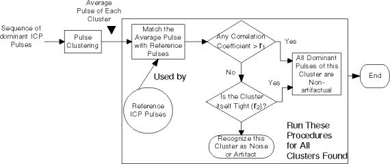
The flow chart of the non-artifactual pulse recognition process. A sequence of dominant intracranial pulses is processed by this process to identify those that are non-artifactual based on a collection of non-artifactual reference pulses. Two algorithm parameters are involved in this processing.
E. Detection of ICP Peaks
Figure 4 illustrates an ICP pulse with a prominent peak. In addition, there are several visually identifiable landmarks on this ICP pulse that do not strictly conform with defining i as a local peak of a signal x if it satisfies xi−1 < xi < xi+1. One can have several optional peak definitions for these landmarks. For simplicity, these landmarks are still called peaks in the present work. Figure 4 shows four possible definitions for these visual landmarks. The common step to apply these definitions to locate ICP peaks is to find the second derivative of ICP pulse. This was accomplished using the parametric algorithm [23]. Based on the sign of (x(n)′′), an ICP pulse curve can be segmented into the concave and the concave regions, which are denoted with circles in Fig. 4. Peak locations,according to four possible definitions, can be found using the concave portions of the pulse curve. The first definition treats the intersection of a concave to a concave region as a peak if the first derivative of the the concave portion is greater than zero otherwise the intersection of a concave region to a concave region is the peak. The second definition is based on the curvature of the signal such that the peak is the location with maximal absolute curvature within each concave region, which can be calculated as the following metric
| (4) |
The third and the fourth definitions both involve a straight line linking the two end points of a concave region. According to the third and the fourth definitions, a peak can be found at the position where the perpendicular distance or the vertical distance from the ICP to this line is maximal, respectively.
Fig. 4.
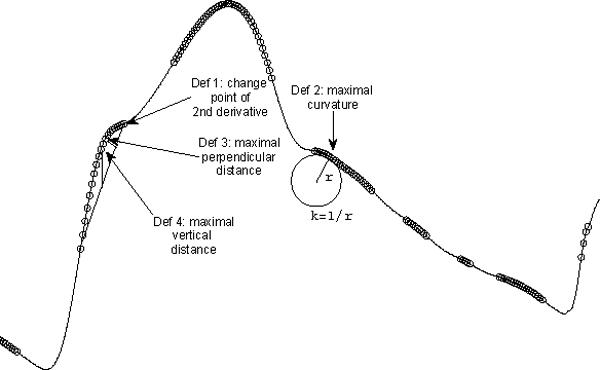
An illustration of four possible extended definitions of ICP peak candidates using a dominant ICP pulse. The portions of the pulse curve that have a negative second order derivative is overlapped with circles. Only the first definition was used in the present work but all definitions are given here for the reason of completeness.
As can be seen in Fig. 4, there are several concave regions in an ICP pulse. One additional constraint we applied is that the first peak should be detected on the rising edge and the last peak should be detected on the descending edge of ICP pulse.
These four peak definitions may have different implications but this topic is beyond the scope of the present work where the first definition was adopted in the process of validating other aspects of the MOCAIP algorithm. However, all definitions are given here for the reason of completeness.
F. Optimal Assignment of Detected Peaks
This is the last step of the MOCAIP. The objective is to obtain the best designation of the three well-recognized ICP peaks, denoted as P1, P2, and P3 respectively, from an array of detected candidate peaks plus an empty designation. Let a1, a2, . . . , aN represent an array of N detected peak candidates and a0 represent an empty designation. In addition, we use Pi(y), i = 1, 2, 3 to denote the probability density functions (PDF) of assigning a candidate point y to Pi. These PDFs were constructed based on the locations of designated ICP peaks for a set of reference ICP pulses assuming a normal distribution of the three peaks.
The criterion for an optimal assignment is to achieve the maximum of the following objective function
| (5) |
subjected to any of the following eight conditions
| (6) |
| (7) |
| (8) |
| (9) |
| (10) |
| (11) |
| (12) |
| (13) |
The first condition denotes that none of peaks is presented. Conditions 2 through 4 represent cases where only one peak is present. Conditions 5 through 7 represent cases where only two peaks are present. All three peaks are present if the last condition is met.
Apparently, J(i, j, k) can be computed separately for each of the constraints. Then the best J(i, j, k) can be selected as the final solution.
It is trivial to evaluate J(i, j, k) for constraints 2 through 4 as one can have each of ai evaluated by the target PDF such that
| (15) |
| (16) |
| (17) |
To obtain J(i, j, k) for the rest of constraints including constraints 5 through 8, one has to additionally consider the order of designating P1, P2, and P3. Let TO (trial order) represent a set of all possible orders of attempting peak assignment for P1, P2, and P3. Hence, TO for the eighth constraint is a 6 × 3 array corresponding to six different orderings of P1, P2, and P3 and it will be a 2 × 2 matrix for constraints 5 through 7. With this definition of TO, we can obtain the optimal J for constraints 5 through 8 as the the following
| (18) |
where the determination of trial order (TO) for each constraint is described above. Lj and Uj are dynamically-determined lower and upper bounds for the search region of akj . Lj is determined as the a(ko+1) where ako is the assignment to the peak that is closest to TOi, j from the below. Uj is determined as the a(ko−1) where ako is the assignment to the peak that is closest to TOi, j from the above.
To avoid false designation, we introduce a parameter ρ such that Pi(ak) = 0, i ∈ {1, 2, 3}, k ∈ {1, 2, . . . , N} if probability of assigning ak to Pi is less than ρ. Therefore, when Pi(ak) = 0 for all i and ak, the first condition will be satisfied and all three peaks will be designated as absent.
G. A baseline peak designation algorithm
As a baseline to compare the proposed optimal peak designation, let us briefly introduce an existing algorithm of peak designation [24]. This algorithm partially solves the peak designation because it only designates peaks for pulses whose number of candidate peaks is greater than three. It relies on two sorting criteria of the peak candidates. The first criterion is based on the amplitudes of the peak candidates and the second is based on their curvatures. All candidate peaks of the pulse are sorted in a descending order based on these two criteria, respectively. If the top three candidates resulted from each criterion match with each other, then these three peaks were taken as the P1, P2, and P3. Otherwise, the algorithm will skip the designation of peaks.
H. Validation Protocol and Patient Data
In the present work, the MOCAIP algorithm will be validated with regard to the following two aspects:
How well does the algorithm recognize non-artifactual dominant pulses?
How accurately does the algorithm designate the three well-recognized ICP peaks?
1) Protocol
Quantitative measures of the above aspects are to be calculated based on a database of continuously acquired ICP and ECG signals using the following protocol. In the following description, we assume that N signal segments were unbiasedly selected in a random fashion from the data archival.
Generate dominant ICP pulses and peak designations using the MOCAIP algorithm. The MOCAIP algorithm will be applied to each of the N signal segments using the set of default algorithm parameters. This will result in a sequence of dominant ICP pulses for each signal segment and their peak designations for the non-artifactual ones.
Build ground truth of dominant ICP pulse recognitions and peak designations. This process is facilitated by utilizing the preliminary results from the above processing. Particularly, each dominant pulse obtained from the above processing will be presented to a human expert. In addition, the peak candidates and the peak designations from the MOCAIP, which can be wrong, will be presented. Using a customized software, the human expert can then decide whether a dominant ICP pulse is non-artifactual and correct the designations of the ICP peaks that were not done correctly by the algorithm. The legitimacy of each dominant pulse and its peak designation after this expert editing process become the ground truth to evaluate the performance of the MOCAIP algorithm in sequel.
Formulate a reference pulse library. Up to 10 non-artifactual dominant ICP pulses from each of the N signal segments will be selected to formulate the reference library. Each entry of the library contains the dominant ICP pulse, the positions of three peaks, and its associated identifier of the patient.
Run the MOCAIP algorithm under different sets of parameters. In applying the MOCAIP to each of the N signal segments, the reference library will be modified accordingly by removing entries from the same patient. To evaluate the performance of the MOCAIP in recognizing non-artifactual dominant pulse, the MOCAIP will be executed for each of the following r1 and r2: r1 ∈ {0.4, 0.5, 0.6, 0.7, 0.80, 0.85, 0.90, 0.92, 0.95, 0.97, 0.99, 0.99, 0 and r2 ∈ {−1, 0.4, 0.6, 0.9, 1}. An r2 = −1 simply indicates that no self-identification will be used. To evaluate the performance of peak designation, the MOCAIP will be executed with different vales of ρ that were obtained as twenty logarithmically equally spaced points from 10−4 to 1.
Calculation of quantitative measures. We use true positive rate (TPR) and false positive rate (FPR) to characterize the performance of the MOCAIP in pulse recognition and peak designation. For pulse recognition, let NTP represent the total number of correctly identified non-artifactual ICP pulse, NFP the number of falsely identified non-artifactual ICP pulses, NTN the number of correctly identified artifactual ICP pulses, and NFN the number of incorrectly identified artifactual ICP pulses. Then its TPR can be calculated as TPR = and its FPR calculated as FPR = . Similar calculation can be done for evaluating the performance of designating each of three ICP peaks.
2) Patient Data
In the present work, N signal segments were selected from the recoded ICP and ECG signals from 66 patients, including 32 females and 34 males, who were seen as inpatients at the UCLA Adult Hydrocephalus Center for various intracranial pressure related conditions. Average age of these patients is 61 with their ages ranging from 14 to 94 years old. During their hospitalization, these patients received continuous intracranial pressure monitoring for the clinical purpose using Codman intraparenchymal microsensors (Codman and Schurtleff, Raynaud, MA) situated in the right frontal lobe. Simultaneous cardiovascular monitoring was also performed using the bedside GE monitors. ICP and lead II of ECG signals were archived using either a mobile cart at the bedside that was equipped with the PowerLab TM SP-16 data acquisition system (ADInstruments, Colorado Springs, CO) or the BedMaster™ system that collects data from the GE Unity network which the bedside monitors were connected to. Majority of signals were recorded using the PowerLab system, which sampled ECG and ICP at 400 Hz. Sampling rate used in the Bedmaster system was 240 Hz. The MOCAIP algorithm handles different sampling rates internally. The usage of this archived data set in the present work was approved by the UCLA Internal Review Board.
Signal files in this archive were transformed into the Chart™ Binary file format for further processing. A total of N = 153 signal segments, each of which is approximately five-hour long, were randomly selected, at an interval of 12 hours, without avoiding noisy regions from these data set. These 153 signal segments were subsequently processed according to the protocol laid out in the above section.
III. Results
A. Characteristics of the reference library
A total of 1435 dominant pulses were randomly selected to form the complete reference library of ICP pulses. The mean ICP of these pulses was 3.1 ± 7.2 mmHg. The mean amplitude of these ICP pulse was 6.6±3.3 mmHg. The distributions of the locations of P1 through P3 relative to the QRS are shown in Fig. 5 together with the estimated normal PDF. Mean P1 location is 189.79 ± 30.54 milliseconds, P2 location is 313.99 ± 45.18 milliseconds, and mean P3 location is 447.30 ± 47.41 milliseconds.
Fig. 5.
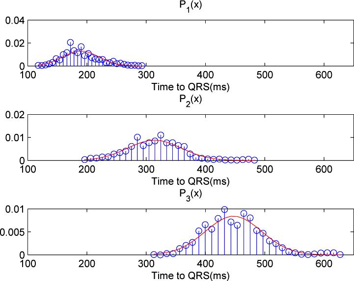
Histograms and the fitted normal probability density function (PDF) of the locations of the three ICP component peaks as determined from the reference library of 1435 ICP dominant pulses.
B. Recognition of non-artifactual dominant ICP pulses
A sequence length of 3 minutes was used in the MOCAIP algorithm, i.e., a dominant ICP pulse was generated for every 3-minute recording. This choice resulted in a total of 14230 raw dominant pulses. The number of non-artifactual dominant pulses was 13371 accounting for 93.96% of identified dominant pulses. The artifactual dominant pulses were caused majorally by noise in the data and by the wrong QRS detections. This high percentage of non-artifactual dominant ICP pulses indicates that clustering a 3-minute sequence of raw ICP effectively removed noise and made the automated analysis of long-term ICP recordings possible. We present three receiver operator characteristic (ROC) curves of recognizing non-artifactual ICP pulse in Fig. 6. These ROC curves were generated under three different configurations of r2. Each ROC curve was generated by systematically changing r1 following r1 ∈ {0.4, 0.5, 0.6, 0.7, 0.80, 0.85, 0.90, 0.92, 0.95, 0.97, 0.99, 0.995}. It can be seen from the figure that adding the self-identification module is important to achieve a good performance without having to carefully choose a proper r1 as a prior while the different choices of r2 had a minimal influence on the performance of recognition of non-artifactual pulses. Particularly, the true positive rate of recognizing non-artifactual pulses was impaired when choosing a high r1 (TPR = 0.84 when r1 = 0.99) and meanwhile disabling self-identification. Figure 7 displays the total accuracy rate of recognizing non-artifactual pulses under the same settings for generating the ROC curves in Fig. 6. Additionally, we provide the baseline accuracy that was obtained by simply recognizing all dominant pulses as non-artifactual. It can be seen from this figure that total accuracy of recognizing non-artifactual pulse is higher without using self identification if proper value for r1 is chosen, e.g., r1 < 0.99 however the adoption of the self-identification makes the algorithm less dependent on a proper choice of r1, which always has a better performance than the baseline.
Fig. 6.
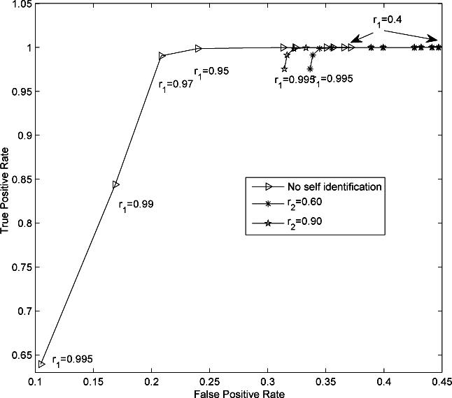
Receiver operator characteristic (ROC) curves of non-artifactual pulse recognition under different r2. Each ROC curve was generated by fixing r2 while systematically changing r1 according to r1 ∈ {0.4, 0.5, 0.6, 0.7, 0.80, 0.85, 0.90, 0.92, 0.95, 0.97, 0.99, 0.995}. It can be seen from the figure that adding the self-identification module is important to achieve a good performance without having to carefully choose a proper r1 as a prior while the different choices of r2 had a minimal influence on the performance of recognition of non-artifactual pulses. Corresponding values of r1 are marked close to several points on the ROC curves. It should be noted that no difference was found in neither true positive nor false positive rate when r1 = 0.4, 0.5, 0.6.
Fig. 7.
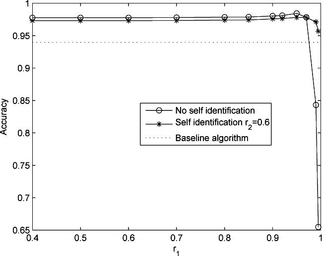
Comparison of accuracies of recognizing non-artifactual pulses at two configurations of r2. Each curve was generated by systematically changing r1 whose value is indicated on the x-axis. The dotted line denotes the baseline accuracy by assigning each dominant pulse as non-artifactual. A useful algorithm has to achieve a better accuracy better than this baseline.
C. Designation of ICP peaks
To remove the influence of pulse recognition on evaluating peak designation, only the true positive pulse recognitions are used in characterizing ROC curves of peak designations. Thus there are a total of 13364 correctly identified non-artifactual dominant pulses. Among these pulses, 1717 have missing P1, 265 have missing P2 and 34 have missing P3. This result indicates that most of the dominant ICP pulses have three distinctive peaks. The average number of peak candidates is 5.67 ± 2.00. Figure 8 shows the ROCs for correctly designating the three ICP peaks. The horizontal line in each plot gives the true positive rate of the baseline algorithm, which we introduced in [24]. False positive rate of this baseline algorithm could not be assessed because only dominant pulses with three peaks can be used to evaluate this baseline algorithm as it did not possess the ability of allocating peaks when the number of peaks present is less than three. It can be seen from this figure that appropriate choice of ρ can result in a superior performance of the MOCAIP algorithm in term of true positive rate. Based on these ROC plots, an optimal choice of ρ was 0.0336, which resulted in a TPR of [91.45%, 88.10%, 86.62%] and a FPR of [18.52%, 38.87%, 52.94%] for correctly designating the three peaks, respectively. A relatively large FPR is justified for this choice because of a low percentage of pulses without a complete set of P1, P2, and P3. In terms of accuracy, this choice resulted in 90.17%, 87.56%, and 86.53% for designating the three peaks, respectively.
Fig. 8.

Receiver operator characteristic curves of designating each of the three ICP component peaks. The horizontal line indicates the performance of the baseline algorithm that did not utilize a library of reference ICP pulses. Each curve was generated by varying ρ that is introduced in Section II-F. Twenty different values for ρ were obtained as 20 logarithmically equally spaced points from 10−4 to 1. We also mark the corresponding ρ values at both ends of a ROC curve.
IV. Discussion
As an effort to create a clinically friendly system of analyzing ICP dynamics for extracting useful information beyond mean ICP, an algorithm capable of detecting and designating individual sub-peaks of ICP pulses from continuous ICP was introduced in the present work. This algorithm creates the potential of automatically and continuously extracting and analyzing morphological features of ICP pulses. An extensive validation of the proposed MOCAIP algorithm was conducted using a dataset from 66 patients with a total monitoring time of about 700 hours. Validation results demonstrate the efficacy of the algorithm. Under optimal parameters as found using the ROC analysis, the MOCAIP algorithm has a true positive rate of 99.04% and a false positive rate of 20.08% in recognizing non-artifactual ICP pulse with a combined accuracy of 97.84%. It also achieved a true positive rate of [91.45%, 88.10%, 86.62%] and a FPR of [18.52%, 38.87%, 52.94%] for correctly designating the three peaks with a combined accuracy of 90.17%, 87.56%, and 86.53%, respectively. Our results also showed that majority of dominant ICP pulses have all three well-recognized ICP peaks having a prevalence rate of 87.15%, 98.02%, and 99.75%, respectively.
A. Existing methods of analyzing ICP pulse morphology
Several methods have been proposed in the past for analyzing ICP pulse morphology. Early ones relied on the changes in the spectral components of ICP pulse to infer temporal changes [13], [25]–[27]. These methods have not been widely adopted in practice and have not been tested using long-term ICP from modern monitoring devices. Computer software, described in a 1995 report [28], appeared to be capable of analyzing single ICP pulse in terms of extracting maxim, minimum, average, amplitude and pulse gradient. However, no description of the methodology was presented. Therefore, it cannot be assessed whether the approach could resolute each individual sub-peak in an ICP pulse. More recently, a method was proposed [5], which demonstrated some potential of extracting useful information from analyzing ICP pulses using a large amount of clinical data. However, the accuracy of this method in analyzing ICP from clinical recordings, which are usually subjected to various noise and artifacts, has not been quantified. In addition, application of this method to analyze peak configuration changes has not been attempted. Another interesting approach of analyzing morphology of ICP has been proposed in [4]. This method emphasized visualization of morphological changes and hence is best suited as an exploratory tool. In addition, it has only been applied to a limited number of cases without considering effects from noise and artifacts.
B. the MOCAIP algorithm
The present work represents a different approach towards analyzing ICP pulse morphological changes. The output of the MOCAIP would appeal to clinical users because intuitive parameters characterizing peak configurations can be readily extracted once the locations of each ICP peak is found. For example, in addition to the features based on amplitudes of peaks, the temporal intervals between peaks can also be utilized to derive useful features. To our knowledge, these interval-based features have not been studied before.
Non-artifactual pulse recognition was demonstrated to be successful with an overall accuracy of 97.84%. This is partly due to the adoption of a reference library of non-artifactual ICP pulses and partly due to the use of the pulse clustering. Designation of the P1, P2, and P3 is more challenging. As a first systematic effort at solving this problem, the MOCAIP algorithm achieved an overall accuracy around 85% for P3 and an accuracy approaching 90% for P1. This may reflect the fact that P2 and P3 have a larger variability and that more candidate peaks are detected at later portions of an ICP pulse. Further pursuing the peak designation problem is necessary to increase the accuracy that could benefit from incorporating additional information from the amplitude or curvature of the peak candidates. Having a reference library proved to be instrumental in achieving good performance of designating ICP peaks as well, not only at situations when the number of candidate peaks was less than three, but also in other more common situations where the number of peak candidates is greater than two. Without using a reference library, the baseline algorithm only achieved an accuracy of 65%.
It should be also noted that the above validation results were obtained using a database of intraparenchymal ICP signals all from hydrocephalic patients. The generalization of reference pulse library to ICP recorded for different disease groups in the ventricular or the subarachnoid space remains to be investigated. The performance of peak designation may be more dependent on the generalizability as compared to that of pulse recognition because the parameters characterizing the statistics of peak locations may be quite different between intraparenchymal ICP recorded for hydrocephalic patients and ventricular ICP recorded for brain injury patients.
C. Future clinical applications
In future clinical investigations of the MOCAIP algorithm, several research venues could be pursued. In neurocritical care settings, the MOCAIP algorithm can be used to process continuous ICP from bedside monitors to extract predictive information that may indicate the progression of dangerous brain structural and cerebral vascular changes including volumetric increase of the ventricles [24], the growth of intracranial lesions, and the development of cerebral vasospasm. Such an research effort could help elucidate further whether the extended ICP monitoring using the MOCAIP could help achieve a real-time recognition of the progression of various types of secondary insult to the brain after the initial stabilization of the primary injury, which is an ultimate goal of having a 24-hour monitoring of patients. Such research effort will involve the corroboration of ICP morphological features with those volumetric or geometric measures from brain imaging studies that are accurate but cannot be assessed in continuous fashion. In addition, a reference pulse library built using ventricular ICP data may be necessary to pursue these studies.
In chronic settings such as diagnosing and treating hydrocephalus patients, the current reference pulse library can be combined with the corresponding patient outcome information to provide diagnostic or prognostic information for better interpreting results from MOCAIP processing. Quantitative clinical decision support for shunt treatment is still a challenge. Some existing reports have shown that recognizing specific ICP patterns in overnight recordings, such as B-waves, may be helpful to offer clues for differentiating between shunt responders and non-responders [29]. Therefore, it can be anticipated that the MOCAIP algorithm could be an enabling technique for automating analysis of overnight ICP recordings that could be useful in predicting whether normal pressure hydrocephalus patients could respond to the shunt treatment.
Our discussion so far has been focused on the analysis of ICP pulse. It should be realized that some of ICP pulse morphological features could be influenced by extracranial factors, e.g., stiffness of the systemic circulation would determine the cerebral arterial pulse morphology from which ICP pulse originates. One should thus be cautious in interpreting the MOCAIP results when having access only to ICP signal. Given the fact that there is no such limitation that the MOCAIP cannot be applied to analyze other pulsatile signals such as arterial blood pressure, it would be beneficial to include systemic pulsatile signals in the data acquisition and analysis. It will be also meaningful to investigate whether certain MOCAIP features such as time intervals between sub-peaks would be immune to extracranial confounding factors. Finally, it should be emphasized that MOCAIP analysis of continuous ICP is a constituent element of a system of extracting diagnostic information from ICP that also includes other data analysis techniques such as machine learning.
V. Conclusion
The MOCAIP algorithm has been demonstrated to be able to accurately identify, from continuous ICP recordings, non-artifactual dominant ICP pulses for analysis and to satisfactorily detect and designate individual peaks in an ICP pulse. These capabilities of the MOCAIP algorithm suggest a great potential for applications in real clinical settings requiring prolonged ICP monitoring.
VI. Acknowledgments
The present work is supported in part by NINDS grants R21-NS055998, R21-NS055045, R21-NS059797 and R01-NS054881.
Biography

Xiao Hu received the B.S. and M.S. from the University of Electronic Science and Technology of China in 1996 and 1999, respectively. He received a Ph.D. degree in Biomedical Engineering from the University of California, Los Angeles in 2004. He joined the division of neurosurgery at the UCLA Medical Center as an assistant researcher in 2004 and then as an assistant professor in December 2006. He has a broad research interest in biomedical modeling, signal processing, and biomedical informatics. He is currently the director of the Neural Systems and Dynamics Laboratory (NSDL).

Peng Xu received the B.S and Ph.D. degrees in biomedical engineering from the University of Electronic Science and Technology of China (UESTC), Chengdu, China in 2000 and 2006, respectively. He is now a visiting fellow at Neural Systems and Dynamics Laboratory, University of California, Los Angeles. His research interest includes biomedical signal processing, biomedical models and medical image analysis.

Fabien Scalzo received the MSc degree and the PhD degree in Computer Science in 2002 and 2007 from the University of Lige in Belgium. In 2007, he was a recipient of a Belgian American Educational Foundation fellowship (BAEF). He subsequently worked as postdoctoral researcher in machine learning and computer vision at the University of Nevada, Reno in 2007, at the University of California, Los Angeles in 2008 and at the University of Rochester, New-York where he is currently. His research interests include machine learning, computer vision and neuroscience.

Paul Vespa is a Professor of Neurology and Neurosurgery at the David Geffen School of Medicine at UCLA. He is the director of the Neurocritical Care program. He is a fellow-elect of the American College of Critical Care Medicine. He has clinical and research interests in traumatic brain injury, intracerebral hemorrhage, status epilepticus, stroke, subarachnoid hemorrhage and coma. Dr. Vespa has pioneered the role of brain monitoring in the neurointensive care unit. He has also pioneered robotic telepresence in the Neuro-ICU. He has published over 68 articles and is an editorial board member of several international journals. Dr. Vespa is funded to do cutting-edge research by the National Institutes of Health and the State of California Neurotrauma Initiative.

Marvin Bergsneider received a B.S. in Electrical Engineering in 1983 from the University of Arizona, followed by a M.D. degree in 1987 from the University of Arizona College of Medicine. He obtained his neurosurgical residency training at UCLA, where he joined the faculty in 1994. He is a Professor of Neurosurgery and a faculty member of the UCLA Biomedical Engineering Interdepartmental Program. His research interests include modeling of intracranial fluid biomechanics and hydrocephalus, plus bioMEMS development.
Contributor Information
Paul Vespa, Paul Vespa (pvespa@mednet.ucla.edu) is with the Neurocritical Care Program, Department of Neurosurgery, University of California, Los Angeles.
Marvin Bergsneider, Marvin Bergsneider (mbergsneider@mednet.ucla.edu) is with the Neural Systems and Dynamics Laboratory, Department of Neurosurgery, University of California, Los Angeles. Tel: (310)825−9207, Fax: (310)206−5234.
REFERENCES
- 1.Hu X, Nenov V, Bergsneider M, Glenn TC, Vespa P, Martin N. Estimation of hidden state variables of the intracranial system using constrained nonlinear kalman filters. IEEE Trans Biomed Eng. 2007;54(4):597–610. doi: 10.1109/TBME.2006.890130. [DOI] [PubMed] [Google Scholar]
- 2.Hu X, Miller C, Vespa P, Bergsneider M. Adaptive computation of approximate entropy and its application in integrative analysis of irregularity of heart rate variability and intracranial pressure signals. Med Eng Phys. 2007 doi: 10.1016/j.medengphy.2007.07.002. [DOI] [PMC free article] [PubMed] [Google Scholar]
- 3.Hu X, Nenov V, Vespa P, Bergsneider M. Characterization of interdependency between intracranial pressure and heart variability signals: a causal spectral measure and a generalized synchronization measure. IEEE Trans Biomed Eng. 2007;54(8):1407–17. doi: 10.1109/TBME.2007.900802. [DOI] [PMC free article] [PubMed] [Google Scholar]
- 4.Ellis T, McNames J, Aboy M. Pulse morphology visualization and analysis with applications in cardiovascular pressure signals. IEEE Trans Biomed Eng. 2007;54(9):1552–9. doi: 10.1109/TBME.2007.892918. [DOI] [PubMed] [Google Scholar]
- 5.Eide PK. A new method for processing of continuous intracranial pressure signals. Med Eng Phys. 2006;28(6):579–87. doi: 10.1016/j.medengphy.2005.09.008. [DOI] [PubMed] [Google Scholar]
- 6.Hornero R, Aboy M, Abasolo D, McNames J, Goldstein B. Interpretation of approximate entropy: analysis of intracranial pressure approximate entropy during acute intracranial hypertension. IEEE Trans Biomed Eng. 2005;52(10):1671–80. doi: 10.1109/TBME.2005.855722. [DOI] [PubMed] [Google Scholar]
- 7.Czosnyka M, Smielewski P, Kirkpatrick P, Laing RJ, Menon D, Pickard JD. Continuous assessment of the cerebral vasomotor reactivity in head injury. Neurosurgery. 1997;41(1):11–7. doi: 10.1097/00006123-199707000-00005. discussion 17−9. [DOI] [PubMed] [Google Scholar]
- 8.Adolph RJ, Fukusumi H, Fowler NO. Origin of cerebrospinal fluid pulsations. Am J Physiol. 1967;212(4):840–6. doi: 10.1152/ajplegacy.1967.212.4.840. [DOI] [PubMed] [Google Scholar]
- 9.Cardoso ER, Rowan JO, Galbraith S. Analysis of the cerebrospinal fluid pulse wave in intracranial pressure. J Neurosurg. 1983;59(5):817–21. doi: 10.3171/jns.1983.59.5.0817. [DOI] [PubMed] [Google Scholar]
- 10.Hamer J, Alberti E, Hoyer S, Wiedemann K. Influence of systemic and cerebral vascular factors on the cerebrospinal fluid pulse waves. J Neurosurg. 1977;46(1):36–45. doi: 10.3171/jns.1977.46.1.0036. [DOI] [PubMed] [Google Scholar]
- 11.Wilkinson HA, Schuman N, Ruggiero J. Nonvolumetric methods of detecting impaired intracranial compliance or reactivity: pulse width and wave form analysis. J Neurosurg. 1979;50(6):758–67. doi: 10.3171/jns.1979.50.6.0758. [DOI] [PubMed] [Google Scholar]
- 12.Chopp M, Portnoy HD. Systems analysis of intracranial pressure. comparison with volume-pressure test and csf-pulse amplitude analysis. J Neurosurg. 1980;53(4):516–27. doi: 10.3171/jns.1980.53.4.0516. [DOI] [PubMed] [Google Scholar]
- 13.Takizawa H, Gabra-Sanders T, Miller JD. Changes in the cerebrospinal fluid pulse wave spectrum associated with raised intracranial pressure. Neurosurgery. 1987;20(3):355–61. doi: 10.1227/00006123-198703000-00001. [DOI] [PubMed] [Google Scholar]
- 14.Contant J, C. F., Robertson CS, Crouch J, Gopinath SP, Narayan RK, Grossman RG. Intracranial pressure waveform indices in transient and refractory intracranial hypertension. J Neurosci Methods. 1995;57(1):15–25. doi: 10.1016/0165-0270(94)00106-q. [DOI] [PubMed] [Google Scholar]
- 15.Portnoy HD, Chopp M, Branch C, Shannon MB. Cerebrospinal fluid pulse waveform as an indicator of cerebral autoregulation. J Neurosurg. 1982;56(5):666–78. doi: 10.3171/jns.1982.56.5.0666. [DOI] [PubMed] [Google Scholar]
- 16.Cardoso ER, Reddy K, Bose D. Effect of subarachnoid hemorrhage on intracranial pulse waves in cats. J Neurosurg. 1988;69(5):712–8. doi: 10.3171/jns.1988.69.5.0712. [DOI] [PubMed] [Google Scholar]
- 17.Portnoy HD, Chopp M. Cerebrospinal fluid pulse wave form analysis during hypercapnia and hypoxia. Neurosurgery. 1981;9(1):14–27. doi: 10.1227/00006123-198107000-00004. [DOI] [PubMed] [Google Scholar]
- 18.Kirkness CJ, Mitchell PH, Burr RL, March KS, Newell DW. Intracranial pressure waveform analysis: clinical and research implications. J Neurosci Nurs. 2000;32(5):271–7. doi: 10.1097/01376517-200010000-00007. [DOI] [PubMed] [Google Scholar]
- 19.Aboy M, McNames J, Thong T, Tsunami D, Ellenby MS, Goldstein B. An automatic beat detection algorithm for pressure signals. IEEE Trans Biomed Eng. 2005;52(10):1662–70. doi: 10.1109/TBME.2005.855725. [DOI] [PubMed] [Google Scholar]
- 20.Afonso VX, Tompkins WJ, Nguyen TQ, Luo S. Ecg beat detection using filter banks. IEEE Trans Biomed Eng. 1999;46(2):192–202. doi: 10.1109/10.740882. [DOI] [PubMed] [Google Scholar]
- 21.Hu X, Xu P, Lee DJ, Vespa P, Baldwin K, Bergsneider M. An algorithm for extracting intracranial pressure latency relative to electrocardiogram r wave. Physiol Meas. 2008;29(4):459–471. doi: 10.1088/0967-3334/29/4/004. [DOI] [PMC free article] [PubMed] [Google Scholar]
- 22.Kaufman L, Rousseeuw PJ. Finding groups in data : an introduction to cluster analysis. Wiley; Hoboken, N.J.: 2005. Wiley series in probability and mathematical statistics. Leonard Kaufman, Peter J. Rousseeuw.
- 23.Rabiner LR, Juang BH. Fundamentals of speech recognition. PTR Prentice Hall; Englewood Cliffs, N.J.: 1993. Prentice Hall signal processing series. Lawrence Rabiner, Biing-Hwang Juang.
- 24.Hu X, Glenn T, Miller C, Lee D, Vespa P, Bergsneider M. Morphological changes of intracranial pressure pulse are correlated with acute dilatation of ventricles. Acta Neurochirurgica Supplement. 2007 doi: 10.1007/978-3-211-85578-2_27. Accepted. [DOI] [PubMed] [Google Scholar]
- 25.Chopp M, Portnoy HD. Analysis of intracranial pressure waveforms, comparison to the volume pressure test. Biomed Sci Instrum. 1980;16:149–58. [PubMed] [Google Scholar]
- 26.Branch C, Chopp M, Portnoy HD. Fast fourier transform of individual cerebrospinal fluid pulse waves. Biomed Sci Instrum. 1981;17:45. [PubMed] [Google Scholar]
- 27.Piper IR, Miller JD, Dearden NM, Leggate JR, Robertson I. Systems analysis of cerebrovascular pressure transmission: an observational study in head-injured patients. J Neurosurg. 1990;73(6):871–80. doi: 10.3171/jns.1990.73.6.0871. [DOI] [PubMed] [Google Scholar]
- 28.Morgalla MH, Stumm F, Hesse G. A computer-based method for continuous single pulse analysis of intracranial pressure waves. J Neurol Sci. 1999;168(2):90–5. doi: 10.1016/s0022-510x(99)00137-9. [DOI] [PubMed] [Google Scholar]
- 29.Symon L, Dorsch NW. Use of long-term intracranial pressure measurement to assess hydrocephalic patients prior to shunt surgery. J Neurosurg. 1975;42(3):258–73. doi: 10.3171/jns.1975.42.3.0258. [DOI] [PubMed] [Google Scholar]