Automatic nonrigid registration of whole body CT mice images

Abstract

Three-dimensional intra- and intersubject registration of image volumes is important for tasks that include quantification of temporal∕longitudinal changes, atlas-based segmentation, computing population averages, or voxel and tensor-based morphometry. While a number of methods have been proposed to address this problem, few have focused on the problem of registering whole body image volumes acquired either from humans or small animals. These image volumes typically contain a large number of articulated structures, which makes registration more difficult than the registration of head images, to which the majority of registration algorithms have been applied. This article presents a new method for the automatic registration of whole body computed tomography (CT) volumes, which consists of two main steps. Skeletons are first brought into approximate correspondence with a robust point-based method. Transformations so obtained are refined with an intensity-based nonrigid registration algorithm that includes spatial adaptation of the transformation’s stiffness. The approach has been applied to whole body CT images of mice, to CT images of the human upper torso, and to human head and neck CT images. To validate the authors method on soft tissue structures, which are difficult to see in CT images, the authors use coregistered magnetic resonance images. They demonstrate that the approach they propose can successfully register image volumes even when these volumes are very different in size and shape or if they have been acquired with the subjects in different positions.

INTRODUCTION

Image registration is essential to quantitatively follow disease progression, to assess response to therapy, to compare populations, or to develop atlas-based segmentation methods. The first two applications typically involve several image volumes acquired serially from the same subject and require intrasubject registration methods. The last two, which involve images acquired from different subjects, require intersubject registration techniques. In both cases, nonrigid registration methods are required as soon as the structures of interest are more complex than a single rigid body object. A number of methods and techniques have been developed to achieve this; chief among them are intensity-based techniques and, in particular, methods that rely on mutual information (MI).^{1, 2} However, most automatic methods that have been proposed have been applied to head images only. This is no doubt due to the fact that whole body image data sets present a set of difficulties not found in head data sets. Head images contain one single major identifiable structure (the brain) as opposed to whole body images that contain many articulated structures (the skeleton and organs). Despite the fact that a number of methods have been proposed for extra-cranial applications such as breast, lung, or prostate images,^{3, 4, 5} very few have been proposed to attack issues associated with images that contain many articulated structures the relative position of which changes between acquisitions.

This type of images remains challenging because, in practice, nonrigid registration algorithms need to be initialized with a rigid or affine transformation. If the image volumes do not contain articulated structures, as is the case, for example, for head images, one global rigid or affine transformation is sufficient to initialize the nonrigid registration algorithms. If, on the other hand, these image volumes contain a number of skeletal structures, which are rigid but whose relative position changes from acquisition to acquisition, one global rigid or affine transformation is insufficient and more local approaches have to be used. We now briefly review the methods designed to address this problem.

A typical approach that is used is to rely on a number of local transformations, each one computed for one element in the articulated structure. These transformations are then combined. This is the approach followed by Little et al.⁶ These authors present a technique designed for the intrasubject registration of head and neck images. Vertebrae are registered to each other using rigid body transformations (one for each pair of vertebrae). Transformations obtained for the vertebrae are then interpolated to produce a transformation for the entire volume. One limitation of this approach is that it requires segmenting and identifying corresponding vertebrae in the image volumes. Because corresponding vertebrae are registered with rigid-body transformations, the approach is also applicable only to intrasubject registration problems.

Martin-Fernandez et al.⁷ proposed a method, which they term “articulated registration.” This approach requires the labeling of landmarks to define wire models that represent the bones. A series of affine transformations are computed to register the rods, which are the elements of the wires. The final transformation for any pixel in the image is obtained as a linear combination of these elementary transformations with a weighting scheme that is inversely proportional to the distance to a specific rod.

Arsigny et al.⁸ also present an approach in which local rigid or affine transformations are combined. They note that simple averaging of these transformations leads to lack of invertibility, and they propose a scheme that permits the combination of these local transformations, while producing an overall invertible one. Their method, which is applied to the registration of histological images, has not been tested on whole body images.

Recently, Papademetris et al.⁹ put forth an articulated rigid registration method that is applied to the serial registration of lower-limb mouse images. In this approach, each individual joint is labeled and the plane in which the axis of rotation for each joint lies is identified. A transformation that blends piecewise rotations is then computed. Their approach produces a transformation that is continuous at these interfaces but requires manual identification of joint segments. The authors have applied their method to the registration of lower limbs in serial mouse images. The same authors have also presented an integrated intensity and point-feature nonrigid registration method that has been used for the registration of sulcal patterns and for the creation of mice population averages.¹⁰ While similar to our own approach, it has not been used for the registration of skeletons.

du Bois d’Aische et al.¹¹ deal with the articulated rigid body registration problem using a three-step strategy: (1) articulated registration which combines a set of rigid body matrices, (2) mesh generation for the image, and (3) propagating the displacement to the whole volume. This work has only been applied to intrasubject registration problems.

Johnson et al.¹² presented two algorithms called consistent landmark thin-plate spline registration and consistent intensity-based thin-plate spline registration. Then they extend these to the consistent landmark and intensity registration algorithm, in order to match both landmarks and the areas away from the landmarks. In this algorithm, the landmarks need to be selected and their correspondences need to be identified manually.

Baiker et al.¹³ introduced a hierarchical anatomical model of the mouse skeleton system for the articulated registration of three-dimensional whole body data of mice. But their model does not include the ribs, which we have found important to guarantee the accurate registration of structures such as the heart or the lungs.

In summary, a survey of the literature shows that only a few methods have been proposed to register images including articulated structures. Most approaches compute piecewise rigid or affine transformations and somehow blend and combine these transformations. Unfortunately, these approaches are often not practical because they require identifying various structures in the images such as joints or individual bones and are therefore not automatic. In this article we propose a fully automatic method that does not require structure labeling. We demonstrate its performance on small animal and human images. The data used in this study are described in Sec. 2 of this article. In Sec. 3, we introduce the whole body image registration method we propose, which includes three main steps. The experiments we have performed and results we have obtained are presented in Sec. 4. Both our algorithm and results are discussed in Sec. 5.

DATA

Two types of images have been used in the study presented herein: images acquired from small animals and images acquired from humans. The small animal data sets include computed tomography (CT) and magnetic resonance (MR) images while the human data sets only include CT images. MR images have been acquired for the small animals to permit validation of the method we propose, which is primarily designed for CT images, on soft tissue structures. Soft tissue contrast in CT images is poor but the additional MR image volumes we have acquired permits to validate indirectly our method, as will be described in more details in Sec. 4.

To permit long MR acquisition times with high signal to noise and without motion artifacts, mice were first sacrificed, and then imaged in a Varian 7.0T MR scanner equipped with a 38 mm quadrature birdcage coil. A T₁-weighted spoiled gradient recalled echo sequence with a TR∕TE of 20 ms∕5 ms and a flip angle of 5° was employed. The acquisition matrix was 500×128×128 over a 90×32×32 field of view yielding a spatial resolution of approximately 0.176×0.25×0.25 mm³. Next the mice were imaged within the same holder using an Imtek MicroCAT II small animal scanner to generate the CT images. CT imaging was at a voltage of 80 kvp with an anode current of 500 μA. Acquisition parameters of 360 projections in 1° steps, exposure time 600 ms, and acquisition matrix 512×512×512 were employed. Total scan time is just over 8 min, and images have 0.2×0.2×0.2 mm³ isotropic voxels. The mice posture was then changed arbitrarily and a second set of MR and CT scans were acquired. This process was repeated in four mice. The CT and corresponding MRI scans for each mouse can easily be coregistered with a rigid body transformation because the mouse was in the same holder during CT and MR acquisitions.

Although our main domain of application is small animal images, we have also used human data sets to show the generality of our algorithm. Two pairs of intersubject human upper torso images were acquired. One pair of images consists in a 512×512×170 and a 512×512×198 CT volumes with a voxel resolution of 0.9375×0.9375×3 mm³. The other pair of images consists in a 512×512×184 and a 512×512×102 CT volumes with a resolution of 0.9375×0.9375×3 mm³ as well.

METHOD

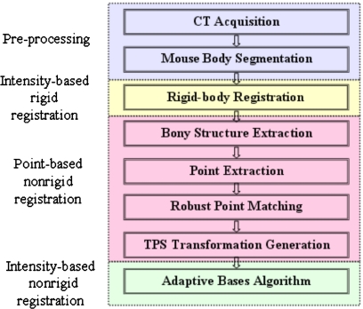
The method we propose involves three main steps (shown in Fig. 1): intensity-based rigid body registration, point-based nonrigid registration, and intensity-based nonrigid registration. These three steps are discussed in detail in the following sections.

Figure 1.

The flow chart of the algorithm, which includes three main steps: intensity-based rigid body registration, point-based nonrigid registration, and intensity-based nonrigid registration.

Step one: Intensity-based rigid body registration

First, a standard MI based rigid body registration algorithm¹⁴ is applied to the source and target CT volumes. A rotation matrix R and a translation vector t, which maximize the normalized mutual information¹⁵ (NMI) between the images are computed using Powell’s conjugate direction method.¹⁶ The normalized mutual information is defined as

$$\text{NMI}=\frac{H\left(A\right)+H\left(B\right)}{H\left(A,B\right)},$$ (1)

where A and B are two images, and H(⋅) is the Shannon entropy of the image which measures the amount of information in this image

$$H\left(A\right)=-\sum _{i\in A}{p}_i\left(i\right)\text{log}{p}_i\left(i\right),$$ (2)

with p_i(i) is the probability of an intensity value i in the image A.

Step two: Nonrigid point-based registration

Next, a set of points is extracted from the skeletons in the images to be registered. In CT images, the bones have a higher intensity than soft tissues. The bony structures can thus be segmented easily in CT images with one single threshold. Here, a simple manual method has been used to select this threshold. Isointensity surfaces were generated with various thresholds and the intensity value that produced the best surface was chosen. Points are then selected automatically in the thresholded image as follows. For each axial slice in the skeleton volume, the connected areas are detected and the center of each of these areas is located. The set of points used for registration is the set of central points, which approximately corresponds to the centerline of the skeletons.

The sets of points extracted from the source and the target images are then registered using the robust point matching algorithm proposed by Chui et al.¹⁷ This algorithm takes two sets of points as input and iteratively computes a correspondence between these points and the transformation that registers them.

First, a correspondence matrix is calculated. Instead of assigning a binary value for every pair of points, a continuous value in the interval [0, 1] is calculated, according to the soft assign algorithm proposed by Gold et al.,¹⁸

$$m_{ai}=\frac{1}{T}\text{exp}\left(-\frac{{\left(x_i-f\left({\upsilon }_a\right)\right)}^T\left(x_i-f\left({\upsilon }_a\right)\right)}{2T}\right),$$ (3)

where V:{υ_a,a=1,2,…,K} and X:{x_i,i=1,2,…,N} are two sets of points from the source and target images. f is the transformation or mapping function, which is used to register the images (more details on this mapping function are provided below). T is called the temperature parameter, which is introduced to simulate physical annealing. In the original article (Chui et al.¹⁷), the suggested initial value for T is 0.5. The annealing schedule for T is T=T⋅r, with r as the annealing rate. A recommended value for r is 0.93. In this work, we have used the recommended values for every volume. The fuzzy correspondence matrix is normalized at each iteration, so that the sum of each row and each column is kept as one. Thus, Eq. 3 establishes a fuzzy correspondence between points in the set V and points in the set X; the fuzziness of the assignment decreases as the algorithm progresses. Major advantages of this fuzzy assignment are that the cardinality of the sets X and V does not need to be equal and that a virtual correspondence between points in these sets can be established using this fuzzy matrix, as explained next.

At each iteration, after the correspondence is determined, a thin plate spline-based nonrigid transformation f is computed, which solves the following least-squares problem:

$$\underset{f}{\text{min}}E\left(f\right)=\underset{f}{\text{min}}\sum _{a=1}^K{\Vert y_a-f\left({\upsilon }_a\right)\Vert }^2+\lambda {\Vert Lf\Vert }^2,$$ (4)

where $y_a={\sum }_{i=1}^N{m}_{ai}{x}_i$ and y_a can be considered as a virtual correspondence for υ_a. This correspondence is computed by weighting all the points in X. L is an operator which measures the smoothness of the thin plate spline transformation. Here the integral of the square of the second order derivative of the mapping function f is used. λ is a regularization parameter that balances the terms. The value of λ also changes from iteration to iteration. Initially a high value is chosen for λ, leading to a smooth transformation. As the algorithm progresses, the correspondence between points becomes crisper and the smoothness constraint is relaxed to increase accuracy. As is the case for the other parameters, the value of λ is modified according to an annealing schedule,

$$\lambda ={\lambda }^{\text{init}}\cdot T,$$ (5)

A recommended value for λ^init is 1, which has also been used here. The correspondence and transformation steps are computed iteratively using Eqs. 3, 4, with the temperature T decreasing. Finally, the transformation computed based on the points is applied to the entire image volume. This deformed volume is then used as the input to the next step.

Step three: Intensity-based nonrigid registration

The last step in our approach relies on an intensity-based registration algorithm we have proposed, which we call ABA for adaptive bases algorithm.¹⁹ This algorithm uses mutual information as the similarity measure and models the deformation field that registers the two images as a linear combination of radial basis functions with finite support,

$$\mathbf{v}\left(\mathbf{x}\right)=\sum _{i=1}^N{\mathbf{c}}_i\Phi \left(\mathbf{x}-{\mathbf{x}}_i\right),$$ (6)

where x is a coordinate vector in R^d, with d being the dimensionality of the images, Φ is one of Wu’s compactly supported positive radial basis functions,²⁰ and the c_i’s are the coefficients of these basis functions. The goal is to find the c_i’s that maximize the mutual information between the images. The optimization process for the coefficients includes a steepest gradient descent algorithm combined with a line minimization algorithm. The steepest gradient descent algorithm determines the direction of the optimization. The line minimization calculates the optimal step in this direction.

In our implementation, the algorithm is applied using a multilevel approach. Here, multilevel includes multiscale and multiresolution. The resolution is related to the spatial resolution of the images. The scale is related to the region of support and the number of basis functions. An image pyramid is created and the registration algorithm is applied at each resolution level. The algorithm is started on a low-resolution image with few basis functions with large support. At each spatial resolution level, the region of support and the number of basis functions are modified. Typically, as the image resolution increases, the region of support is decreased and the number of basis function is increased. As a consequence, the transformations become more and more local as the algorithm progresses.

In our experiments, three resolution levels are used in all small animal CT images (64×64×64, 128×128×128, and 256×256×256 voxels). At the lowest level we use a matrix of 6×6×6 basis functions. At the intermediate level, we use a matrix of 10×10×10 basis functions. At the highest resolution level we start with a matrix of 14×14×14 basis functions and then use a matrix of 18×18×18 basis functions. For the two human data sets, three resolution levels are also used: 64×64×50, 128×128×99, and 256×256×198 voxels for the first data set, and 64×64×25, 128×128×51, and 256×256×102 voxels for the second data set (the dimension depend on the dimensions of the original data sets). At the lowest level, 4×4×4, and then 8×8×8 matrices of basis function were used. At the intermediate level, we used first a matrix of 12×12×10 and then a matrix of 16×16×12 basis functions. At the highest resolution, we used 20×20×14, 26×26×16, and 32×32×20 matrices of basis functions. All those parameters were selected experimentally. Practically, parameters are determined once for one type of image and then used without modification to register similar images.

One feature that distinguishes our algorithm from others (see, for instance, Rueckert et al.⁴) is the fact that we do not work on a regular grid. Rather, areas of mismatch are identified and the deformation field is adjusted only on these identified regions. This is done as follows. When the algorithm moves from one level to the other, a regular grid of basis function is placed first on the images. The gradient of the similarity measure with respect to the coefficients of the basis functions is then computed. The location of the basis functions for which this gradient is above a predetermined threshold is used to determine areas of mismatch. The rationale for this choice is that if the gradient is low, either the images are matched well because we have reached a maximum or the information content in this region is low. In either case, trying to modify the transformation in these regions is not productive. Optimization is then performed locally on the identified regions (more details on this approach can be found in Rohde et al.¹⁹).

The algorithm progresses until the highest image resolution and highest scale are reached. Hence, the final deformation field v is computed as

$$\mathbf{v}\left(\mathbf{x}\right)={\mathbf{v}}_1\left(\mathbf{x}\right)+\cdots +{\mathbf{v}}_M\left(\mathbf{x}\right),$$ (7)

where M is the total number of levels. Furthermore, we compute both the forward and the backward transformations simultaneously, and we constrain these transformations to be inverses of each other using the method proposed by Burr.²¹ Although this cannot be proven analytically, experience has shown that the inverse consistency error we achieve with this approach is well below the voxels’ dimension. In our experience, enforcing inverse consistency improves the smoothness and regularity of the transformations.

One important objective of a nonrigid registration algorithm is to produce transformations that are topologically correct (i.e., transformations that do not include tearing or folding). This is difficult to guarantee and it is often implemented by constraining the transformation (e.g., adding a penalty term that is proportional to the second derivative of the deformations field⁴). Here, we follow the same approach, but the field is regularized by constraining the difference between the coefficients of adjacent basis functions (the c_i’s) using a threshold ε. The concept is simple: if the coefficients of adjacent basis functions vary widely, the resulting deformation field changes rapidly. This can be useful as it permits computing transformations that require large local displacements but it may also produce transformations that are ill-behaved. Thus, the threshold ε can be used to control the regularity and the stiffness properties of the transformation. Small values produce smooth transformations that are relatively stiff. Large values lead to transformations that are more elastic but less regular.

This threshold can also be used to vary spatially the properties of the transformations, which is of importance for the application described in this article (in the past we have used the same technique to register images with large space-occupying lesions²²). Indeed, there are two broad categories of structures in the images we need to register: bones and soft tissues. The amount of deformation typically observed for bony and soft tissue structures is very different and the transformations should reflect this fact; they should be stiffer for bony structures than for soft tissue structures. To create spatially varying stiffness properties, a stiffness map is generated. This stiffness map has the same dimensions as the original images and associates a value for ε with each pixel. In this work, we identify bony regions by thresholding the images as described earlier. We then associate a small ε value to bony regions and a large ε value to the other areas in the stiffness map. Experimentally, we have selected 0.01 for the bony region and 0.3 for the other regions, and we use these values for all the volumes presented here.

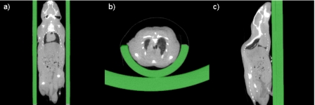
As described before, we have tested our method on two very different sets of data: small animal images and human images. When processing the small animal images, we need to add an additional step to our processing sequence. Indeed, mice are typically scanned in some type of holder and this holder needs to be eliminated prior to registration (see Fig. 2). Manual segmentation is time consuming and impractical, considering the fact that one CT volume usually includes 512 slices. But automatic segmentation using common techniques such as thresholding is difficult. This is so because the intensity values of the mouse and of the holder are very similar and because the body of the mouse is connected tightly to the holder. Here, we solve the problem by segmenting the holder via registration. An empty holder is scanned and registered to the holder that contains a mouse using a normalized mutual information based rigid body registration algorithm.¹⁴ After registration, the image with the empty holder is subtracted from the image with the mouse and the holder. This results in an image, which only contains the mouse. Figure 2 shows representative results in the sagittal, axial, and coronal orientations for a typical mouse CT image volume. This method is fully automatic and robust. It can be used with any type of holder provided that one image volume with an empty holder is available.

Figure 2.

The CT images with segmented holder. The holder is segmented automatically via registration.

EXPERIMENTS AND RESULTS

Qualitative results

Our approach has been qualitatively evaluated on three types of problems: intrasubject registration of whole body mouse images, intersubject registration of whole body mouse images, and intersubject registration of upper body human images. Examples of results obtained for each of these tasks are shown in this section.

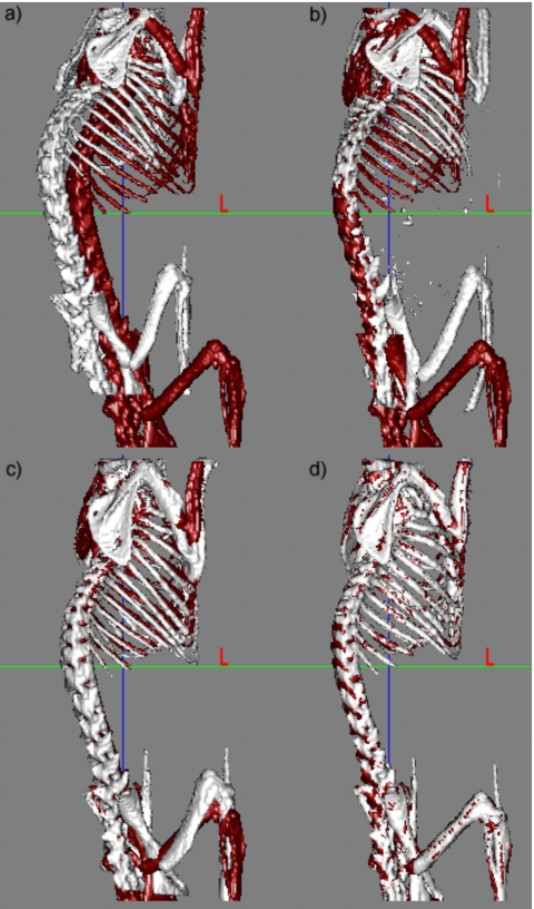
Figure 3a shows the skeletons extracted from two CT volumes; one skeleton is shown in light color, the other in dark color. In the following text the volume that is deformed using our registration method is called the source volume while the other is called the target volume. Figure 3b shows the results we obtain when we use only the ABA algorithm after the initial rigid body transformation. In this case, the algorithm is applied to the entire image volume, and the bones are extracted after registration. This figure shows that for this data set, an intensity-based nonrigid registration algorithm alone is insufficient to register the two volumes. Figure 3c shows the results obtained after registering the skeleton with the point-based method alone. Figure 3d shows the final results when the ABA algorithm is initialized with the results obtained in Fig. 3c. Results presented in this figure indicate that the point-based method leads to qualitatively good results, but that these results can be improved further with an intensity-based technique.

Figure 3.

Bony structures in two micro-CT volumes (a) before registration, (b) after ABA registration only, (c) using only the robust point-based registration algorithm, and (d) using both the point-based registration and the ABA algorithms.

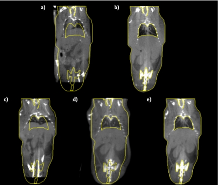
Figure 4 presents similar results but on the entire volume; Fig. 4a shows one slice in the source volume and Fig. 4b shows the slice with the same index in the target volume. If the source and target volumes were perfectly registered, these images would be identical. To facilitate the comparison, yellow contours have been drawn on the target image and copied on all the other ones. Figure 4c shows the results when only ABA is used, Fig. 4d when only the point-based method is used, and Fig. 4e when both methods are combined. Comparing Figs. 4d, 4e it is clear that even if the bones are registered correctly with the point-based technique, the rest of the body is not. For instance, the contour of the lower portion of the mouse body shown in Fig. 4d is not aligned to the target accurately. Again, combining the two methods leads to results that are better than those obtained with a single method.

Figure 4.

(a) One coronal slice in the source volume, (b) the corresponding coronal slice in the target volume, (c) the transformed source image after ABA only, (d) the transformed image after robust point-based registration algorithm only, and (e) the transformed image after the combination of the point-based registration and the ABA algorithms.

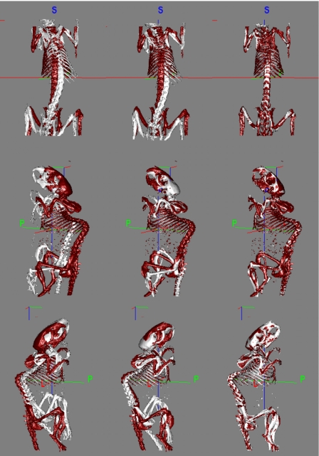
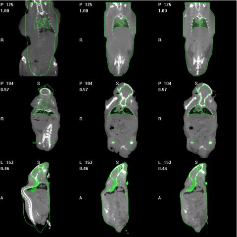
Figures 56 show typical intersubject registration results. In both these figures three pairs of images pertaining to different mice have been registered. Figure 5 shows the registration of the skeletons. In this figure, the left column shows the skeletons in their original position. The middle and right columns show the same but after rigid body registration and after registration with the proposed method, respectively. Figure 6 shows the results we obtain on the entire CT volume. The left column shows one slice in the source volume and the right column shows the same slice in the target volume. The middle column shows this slice in the source volume once it has been registered and reformatted to correspond to the target volume. Contours have been drawn on the target volume and superimposed on the reformatted source volume to show the quality of the registration.

Figure 5.

Three pairs of intersubject mice skeletons before registration (the first column), after rigid body registration (the second column), and after the proposed method (the third column).

Figure 6.

Different slices in three different reference mice (the first column), the deformed slices after the proposed method (the second column), and the corresponding target mice (the third column). The bright lines are contours drawn on the target images.

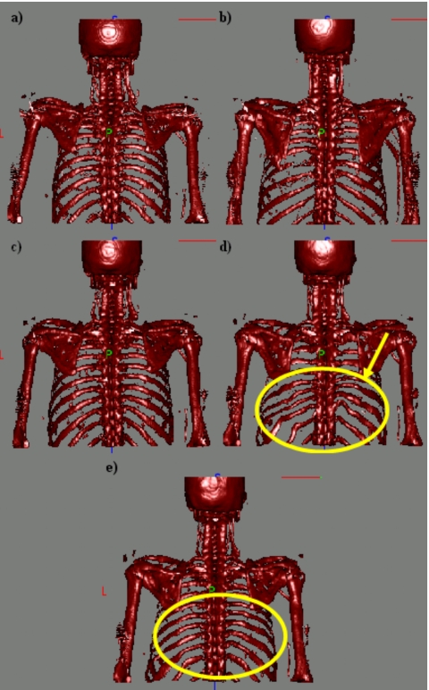
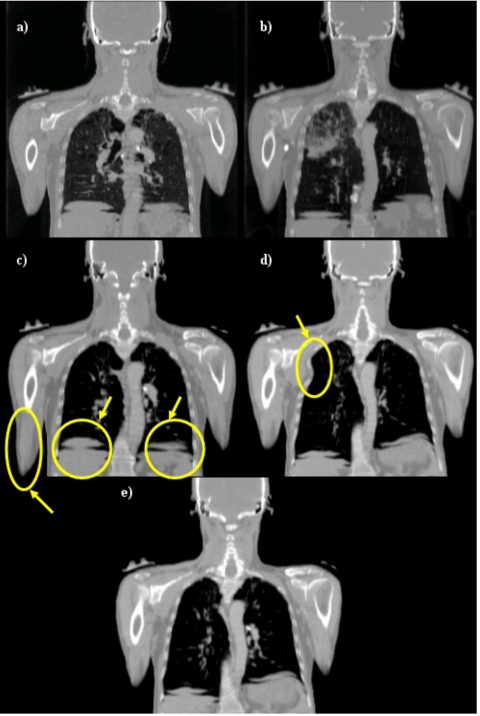
Figures 78 show results we have obtained when performing intersubject registration of human upper torso CT images, and they illustrate the advantage of using two stiffness values. In both figures, panels (a) and (b) are the source images and the target images, respectively. Panels (c), (d), and (e) show the source volume registered to the target volume using a stiff transformation, a very elastic transformation, and a transformation with two stiffness values, respectively. In Fig. 7, only the bones are shown. In Fig. 8, the complete volumes are shown. When a stiff transformation is used, bones are deformed in physically plausible ways. But the accuracy achieved for soft tissues is suboptimal [arrows on Fig. 8c]. When a more elastic transformation is used, bones are deformed incorrectly [shown in Fig. 7d]. Using two stiffness values permits transformations to be computed that lead to more satisfactory results for both the bony and soft tissue regions.

Figure 7.

(a) Skeleton of the source image, (b) skeleton of the target image, (c), (d), and (e) source skeleton registered to target skeleton using a stiff transformation, a very elastic transformation, and two stiffness values, respectively.

Figure 8.

(a) One coronal slice in the source volume, (b) corresponding slice in the target volume, (c), (d), and (e) source image registered to target image using a stiff transformation, a very elastic transformation, and two stiffness values, respectively.

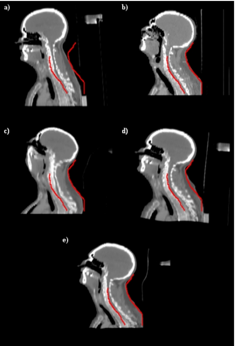
Figure 9 illustrates results we have obtained with a set of head and neck images. Figures 9a, 9b show one sagittal CT image in one of the volumes (the source) and the slice with the same index in the second volume (the target) prior to registration. The contour has been drawn on the target image in order to facilitate comparison. Figures 9c, 9d, 9e show results obtained with our intensity-based algorithm alone, results obtained with point-based registration alone, and results obtained when both approaches are combined, respectively. Figure 9c shows typical results obtained when nonrigid registration algorithms cannot be initialized correctly. The overall shape of the registered volume appears correct but bones have been deformed incorrectly. A closer inspection of the deformation field (not shown here because of space constraints) also shows that the deformation field is very irregular. The deformation field obtained with the point-based registration is smooth but the registration is relatively inaccurate, as shown in Fig. 9d. As can be seen in this panel, the shape of the head and its size are not the same as those shown in Fig. 9b. Similarly, the size of the vertebrae is incorrect. Figure 9e shows that the best results are obtained when both approaches are combined.

Figure 9.

(a) One sagittal slice in the source volume, (b) the corresponding slice in the target volume, (c), (d), and (e) registration results obtained with intensities alone, points alone, and with the proposed algorithm, respectively.

Visual and qualitative validation of our approach indicates that it can be used to register whole body images. To validate this approach quantitatively, we have devised two experiments, one to test the algorithm on the skeletons and the other on soft tissue regions.

Quantitative validation

The acquired data sets, described in Sec. 2, can be used to validate our method both on the skeletons and on soft tissue structures of the same mouse acquired twice in a different posture (longitudinal study) or of two different mice (intersubject registration). We have four pairs of images to test our algorithm on intrasubject longitudinal tasks, e.g., mouse 1 acquired at time 1 is paired with mouse 1 acquired at time 2, etc. With the data set we have acquired, 24 pairs of images can be created to validate our algorithm on intersubject tasks, i.e., mouse 1 at time 1 can be paired with mouse 2 at time 1, with mouse 2 at time 2, etc. Among these 24 pairs, 7 had to be eliminated because one of the data set covered the entire body while the other was missing the lower legs. This leaves us with 17 pairs of images to perform our intersubject evaluation.

Because of acquisition artifacts, the boundary between the heart and the lungs could not bee seen at all in one of the mice (mouse No. 3) CT volumes. In turn, this led to an inaccurate registration in this region when CT images alone were used. For this reason, mouse No. 3 was omitted for the quantitative evaluation of the heart. Validation results on both skeletons and soft tissues are reported in the following sections.

Validation on skeletons

To validate the algorithm on skeletons, the distance between each point on the deformed source surface and the closest point on the target surface is computed. Table 1 shows these distances at each step of the algorithm for both the longitudinal and the intersubject registrations tasks. Hence, the distances are calculated before and after the rigid body registration, after the point matching algorithm, and after the intensity-based nonrigid registration. After the proposed algorithm, the mean distance for the intrasubject registration task is 0.24 mm. It is 0.3 mm for the intersubject registration task. Because the inter-registration task involves accounting for morphological differences in addition to pose differences, observing a slightly larger error for the second task is to be expected.

Table 1.

Distances in mm between the source and target bone surfaces before rigid registration, after rigid registration, after registration using points only, and with the method we propose for both the intra- and intersubject registration tasks.

Mouse No.	Before rigid	After rigid	After point matching	Proposed method
Intrasubject
1	1.7667	0.8175	0.4854	0.3008
2	0.6254	0.4151	0.3853	0.3290
3	0.8205	0.6778	0.2542	0.1422
4	0.7757	0.7164	0.4128	0.2080
Mean	0.9971	0.6567	0.3844	0.245
Intersubject
1	2.4047	1.0170	0.7313	0.4368
2	2.2495	0.4799	0.4964	0.1769
3	1.5536	0.9060	0.5390	0.2530
4	1.0805	0.5425	0.5289	0.2054
5	2.6875	0.5525	0.464	0.2433
6	2.5321	0.5983	0.5878	0.3550
7	2.1083	0.6605	0.7416	0.3255
8	1.2474	0.6147	0.5736	0.2330
9	0.7904	0.5203	0.6069	0.2496
10	1.3014	1.2376	0.4989	0.3300
11	1.1262	1.0090	0.4056	0.2666
12	3.1736	1.0154	0.5111	0.3314
13	2.8424	1.0267	0.5936	0.3795
14	1.9231	0.8696	0.5501	0.3168
15	2.1204	0.9429	0.5337	0.2999
16	2.4757	0.9207	0.6521	0.3734
17	2.2350	0.7434	0.5715	0.3370
Mean	1.9913	0.8034	0.5639	0.3008

Validation on soft tissue structures

The approach we have used to test our registration method on soft tissues both for the intrasubject and the intersubject registration tasks is as follows.

Step (1): each magnetic resonance imaging (MRI) scan was registered to its corresponding CT scan with a rigid transformation;

Step (2): CT scans were then registered using the method we propose;

Step (3): the transformation computed in step (2) was applied to the MRI scans. This permits evaluating the quality of the CT-based registration on structures that are not clearly visible in the CT images.

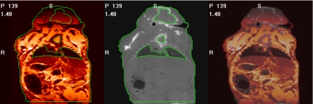
Step (1) in this process is a simple problem. Mice are dead and placed in a holder. This holder is then moved from one scanner to the other without removing the mouse. Registering the two data sets thus only requires computing a rigid body transformation between two data sets in which no or minimum nonrigid displacement can be expected. This is done using a standard mutual information-based rigid body registration algorithm.¹ The accuracy of this registration step has been evaluated qualitatively by blending the registered MR and CT volumes and identifying structures visible in both images, such as the contour of the lungs. A representative example is shown in Fig. 10. The left panel in this figure is a color-coded MR image and the middle panel is the corresponding CT slice. Contours have been drawn on the CT images and copied on the MR images. The right panel shows an image in which the CT and MR images have been blended. In every case, the registration was deemed acceptable. In addition to this visual validation, whole body surfaces were extracted from the MR and CT image volumes after registration with an intensity threshold. For each MR surface point, the closest point on the CT surface was found and its distance to the MR point computed. As shown in Fig. 10, the intensity is attenuated in the top and bottom portions of the MR images. These regions were omitted when computing the distance between the MR and CT surfaces. Table 2 lists the average surface distances for all pairs of MR and CT images used in the experiments described herein. With an overall mean of 0.23 mm, these numbers indicate excellent MR-CT registration results.

Figure 10.

One MR image (left), the corresponding CT image (middle), and the fused image between MR and CT images (right). The bright lines are contours drawn on the CT image and copied to the MR image.

Table 2.

Distances in mm between the source and target mouse body surfaces at different acquisition time points.

MRI-CT surface distance	Mouse No. 1	Mouse No. 2	Mouse No. 3	Mouse No. 4
Time 1	0.1851	0.2659	0.2267	0.2927
Time 2	0.1518	0.2583	0.2234	0.2636

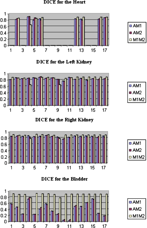
Next, the heart, kidneys, and bladder were segmented manually in all the MR image volumes. The transformations generated by the proposed method were then applied to the structures segmented in the source image. This produced deformed structures that were compared to the segmented structures in each of the target images using the Dice similarity index²³ defined as

$$\text{Dice}\text{similarity}=2\times \frac{n\left\{A_1\cap A_2\right\}}{n\left\{A_1\right\}+n\left\{A_2\right\}},$$ (8)

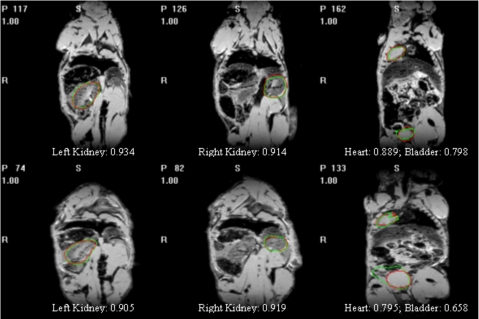
where A₁ and A₂ are two regions and n{⋅} is the number of voxels in a region. Figure 11 shows a few examples with manual and automatic contours superimposed. It also shows the value of the Dice index computed for these various cases to provide a sense of the correlation between the Dice value and the visual quality of the segmentation. A value of 0.7 for the Dice value is customarily accepted as a value for which two contours are in very good correspondence.²⁴

Figure 11.

The target images overlaid with contours obtained automatically and manually.

Two observers have segmented soft tissue structures in the images. Hence, three Dice values are computed and compared: the Dice value between the automatic contours and the manual contours drawn by the first observer, which we call AM1; the Dice values between the automatic contours and the manual contours drawn by the second observer, which we call AM2; and the Dice values between the contours drawn by the two observers, which we call M1M2. The value of the Dice similarity measure between two observers quantifies the inter-rater variability that can be expected for the various segmentation tasks. Although, as discussed above, our main objective is to develop a method for the registration of CT images, we also investigated whether or not using the MR images in the registration process would improve the results. To do so, we added one registration step. After the MR images have been registered to each other using the transformation generated to register the CT images, we registered them once more with the ABA algorithm.

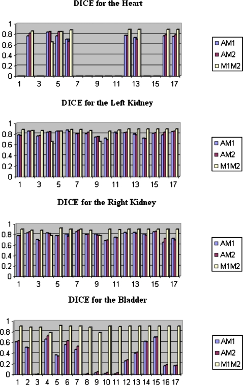
Table 3 lists the Dice values for the longitudinal registration task with and without the last MR registration step. Our results show that Dice values are above 0.7 for the longitudinal registration task. Moreover, the Dice values between the automatic and manual contours are comparable to the Dice values between the two observers, which indicates that the variability between manual and automatic contours is similar to the variability observed between human raters. Figures 1213 show the results for the intersubject registration tasks. For both the intra- and intersubject registration tasks, the Dice values improve when the MR images are used. We also note that the bladder is the most difficult structure to register because of large intersubject differences. This is most likely due to the volume of urine that is present in the bladder at the time of imaging.

Table 3.

Dice similarity values between the two manual segmentations (M1M2), between the first manual segmentation and the automatic segmentation (AM1), and between the second manual segmentation and the automatic one (AM2) for the intrasubject registration task.

Mouse		Heart	Left kidney	Right kidney	Bladder
The proposed method
No. 1	AM1	0.9040	0.9150	0.8730	0.8120
	AM2	0.7997	0.8374	0.7699	0.7213
	M1M2	0.8758	0.9033	0.8958	0.8907
No. 2	AM1	0.8530	0.8930	0.8840	0.8860
	AM2	0.8518	0.8926	0.8649	0.8529
	M1M2	0.8624	0.8810	0.8721	0.8707
No. 3	AM1		0.8820	0.8520	0.7100
	AM2		0.8710	0.9103	0.7708
	M1M2		0.8966	0.8706	0.8364
No. 4	AM1	0.8930	0.8900	0.8860	0.8040
	AM2	0.8684	0.9080	0.8646	0.7752
	M1M2	0.8458	0.9152	0.8878	0.8869
Mean	AM1	0.8833	0.8950	0.8738	0.8030
	AM2	0.8400	0.8772	0.8524	0.7801
	M1M2	0.8613	0.8990	0.8816	0.8712
The proposed method + the extra step
No. 1	AM1	0.9220	0.9090	0.9180	0.7730
	AM2	0.7714	0.8055	0.7582	0.7393
	M1M2	0.8758	0.9033	0.8958	0.8907
No. 2	AM1	0.9200	0.9230	0.9330	0.9510
	AM2	0.8987	0.9114	0.9002	0.8802
	M1M2	0.8624	0.8810	0.8721	0.8707
No. 3	AM1		0.9040	0.8890	0.7650
	AM2		0.8965	0.9111	0.8020
	M1M2		0.8966	0.8706	0.8364
No. 4	AM1	0.9160	0.9120	0.9230	0.8980
	AM2	0.8765	0.9212	0.8984	0.8553
	M1M2	0.8458	0.9152	0.8878	0.8869
Mean	AM1	0.9193	0.9120	0.9158	0.8468
	AM2	0.8489	0.8837	0.8670	0.8192
	M1M2	0.8613	0.8990	0.8816	0.8712

Figure 12.

Dice values for the intersubject registration task without the last MR registration step.

Figure 13.

Dice values for the intersubject registration task with the last MR registration step.

DISCUSSION AND CONCLUSIONS

In this article, we presented a novel and fully automatic approach for the registration of articulated structures applicable to intra- and intersubject registration problems. While it may appear, at first, that registering articulated structures would require computing individual transformations for each element in the structure and combining these transformations, our experiments show that it is not the case. This is what differentiates our work from previously published work and it may have a significant impact because it greatly simplifies the solution to the problem. In particular, segmentation and identification of individual structure components is no longer necessary.

Results have shown that, while accurate registration of bony structures is possible with a robust point-matching method, registration of the entire volumes requires a second step. If, as is done in this work, the second step is based on an image intensity algorithm, special care needs to be taken to constrain the transformation locally to avoid deforming the bony structures inappropriately while registering the rest of the image volumes. Here we have addressed the issue with what we call stiffness maps that constrains the relative value of the coefficients of adjacent basis functions. We have found this scheme to be particularly useful for human images but less so for small animal images. This is so because basis functions have a predetermined support and may cover a region that contains both bones and soft tissue; this is especially true for small animal images in which bones are small compared to the voxel dimensions. In the current version of our nonrigid registration algorithm, we use the position of the center of the basis function to determine its constraint; which may produce inaccuracies, i.e., soft tissue close to the bones may not be deformed enough if the basis functions is centered on a bony structure or bones may be deformed too much if the basis function is centered on soft tissue. We are currently addressing this issue by adding an additional constraint in our algorithm that will prevent this from happening.

The results we have obtained on the skeletons show a submillimetric error for both the serial and the intersubject registration task. The Dice values we have obtained with our approach using only CT images for the intrasubject registration task indicate an excellent agreement between manual and automatic contours. These results indicate that the method we propose could be used for longitudinal measurements using only CT images. A possible issue, which will need to be investigated further, is the effect a growing tumor will have on the intensity-based component of our approach. This may necessitate adapting the stiffness constraints as was done in Duay et al.²² The intersubject registration results we have obtained imply that CT images alone, with their relatively poor soft tissue contrast, may not be sufficient to produce registrations that are accurate enough to measure small differences. Using MR images in addition to the CT images does, however, address the issue. One also notes that using MR images alone is unlikely to produce accurate results. Indeed, the skeletons that are easily identifiable in the CT images need to be used to produce transformations that are accurate enough to initialize MR-based registration algorithms.

Although we have focused our work on CT images of small animals, the results we present also show that the approach we propose is widely applicable. For instance, we have shown, albeit on a few cases, that it can be used for the registration of chest and head and neck images. Further evaluation on a larger data set will need to be performed to establish the robustness of our approach to this type of problem.

For the small animal studies, the average runtime of the robust point matching algorithm is 171 min. The average runtime of the adaptive basis algorithm is 89 min. All algorithms are run on a 2 GHz Pentium PC with 1 G memory.

References

- Maes F., Collignon A., Vandermeulen D., Marchal G., and Suetens P., “Multimodality image registration by maximization of mutual information,” IEEE Trans. Med. Imaging 10.1109/42.563664 16, 187–198 (1997). [DOI] [PubMed] [Google Scholar]
- W. M.WellsIII, Viola P., Atsumi H., Nakajima S., and Kikinis R., “Multi-modal volume registration by maximization of mutual information,” Med. Image Anal. 10.1016/S1361-8415(01)80004-9 1, 35–51 (1996). [DOI] [PubMed] [Google Scholar]
- Camara O., Delso G., and Bloch I., “Free form deformations guided by gradient vector flow: A surface registration method in thoracic and abdominal PET-CT applications,” Workshop in Biomedical Image Registration (WBIR’03), 2003, pp. 224–233.
- Rueckert D., Sonoda L., Hayes C., Hill D., Leach M., and Hawkes D., “Non-rigid registration using free-form deformations: Application to breast MR images,” IEEE Trans. Med. Imaging 10.1109/42.796284 18, 712–721 (1999). [DOI] [PubMed] [Google Scholar]
- Cai J., Chu J. C. H., Recine D., Sharma M., Nguyen C., Rodebaugh R., Saxena V., and Ali A., “CT and PET lung image registration and fusion in radiotherapy treatment planning using Chamfer matching method,” Int. J. Radiat. Oncol., Biol., Phys. 10.1016/S0360-3016(98)00399-X 43, 883–891 (1999). [DOI] [PubMed] [Google Scholar]
- Little J. A., Hill D. L. G., and Hawkes D. J., “Deformations incorporating rigid structures,” Comput. Vis. Image Underst. 10.1006/cviu.1997.0608 66, 223–232 (1997). [DOI] [Google Scholar]
- Martin-Fernandez M., Munoz-Moreno E., Martin-Fernandez M., and Alberola-Lopez C., “Articulated registration: Elastic registration based on a wire-model,” Proc. SPIE 5747, 182–191 (2005). [Google Scholar]
- Arsigny V., Pennec X., and Ayache N., “Polyrigid and polyaffine transformations: A new class of diffeomorphisms for locally rigid or affine registration,” Lect. Notes Comput. Sci. 2879, 829–837 (2003). [Google Scholar]
- Papademetris X., Dione D. P., Dobrucki L. W., Staib L. H., and Sinusas A. J., “Articulated rigid registration for serial lower-limb mouse imaging,” Proceedings of MICCAI’05, 2005, pp. 919–926. [DOI] [PubMed]
- Papademetris X., Jackowski A., Schultz R. T., Staib L. H., and Duncan J. S., “Integrated intensity and point-feature nonrigid registration,” Proceedings of MICCAI’04, 2004, pp. 763–770. [DOI] [PMC free article] [PubMed]
- du Bois d’Aische A., De Craene M., Macq B., and Warfield S. K., “An articulated registration method,” IEEE International Conference on Image Processing (ICIP), 2005, I-21–4. [DOI] [PubMed]
- Johnson H. J. and Christensen G. E., “Consistent landmark and intensity-based image registration,” IEEE Trans. Med. Imaging 10.1109/TMI.2002.1009381 21, 450–461 (2002). [DOI] [PubMed] [Google Scholar]
- Baiker M., Milles J., Vossepoel A. M., Que I., Kaijzel E. L., Lowik C. W. G. M., Reiber J. H. C., Dijkstra J., and Lelieveldt B. P. F., “Fully automated whole-body registration in mice using articulated skeleton atlas,” IEEE International Symposium on Biomedical Imaging (ISBI): From Nano to Macro, 2007, pp. 728–731.
- Studholme C., Hill D. L. G., and Hawkes D. J., “An overlap invariant entropy measure of 3D medical image alignment,” Pattern Recogn. 10.1016/S0031-3203(98)00091-0 32, 71–86 (1999). [DOI] [Google Scholar]
- Press W., Teukolsky S., Vetterling W., and Flannery B., “Numerical Recipes in C,” The Art of Scientific Computing, 2nd ed. (Cambridge University Press, Cambridge, 1994). [Google Scholar]
- Chui H. and Rangarajan A., “A new point matching algorithm for non-rigid registration,” Comput. Vis. Image Underst. 10.1016/S1077-3142(03)00009-2 89, 114–141 (2003). [DOI] [Google Scholar]
- Gold S., Rangarajan A., Lu C. P., Pappu S., and Mjolsness E., “New algorithms for 2D and 3D point matching: pose estimation and correspondence,” Pattern Recogn. 10.1016/S0031-3203(98)80010-1 31, 1019–1031 (1998). [DOI] [Google Scholar]
- Rohde G. K., Aldroubi A., and Dawant B., “The adaptive bases algorithm for intensity-based nonrigid image registration,” IEEE Trans. Med. Imaging 10.1109/TMI.2003.819299 22, 1470–1479 (2003). [DOI] [PubMed] [Google Scholar]
- Wu Z., “Multivariate compactly supported positive definite radial functions,” Adv. Comput. Math. 4, 283–292 (1995). [Google Scholar]
- Burr D. J., “A dynamic model for image registration,” Comput. Graph. Image Process. 15, 102–112 (1981). [Google Scholar]
- Duay V., D’Haese P., Li R, Dawant B M., “Non-rigid registration algorithm with spatially varying stiffness properties,” ISBI, 2004, pp. 408–411.
- Zijdenbos A. P., Dawant B. M., Margolin R. A., and Palmer A. C., “Morphometric analysis of white matter lesions in MR images: Method and validation,” IEEE Trans. Med. Imaging 10.1109/42.363096 13, 716–724 (1994). [DOI] [PubMed] [Google Scholar]
- Bartko J. J., “Measurement and reliability: Statistical thinking considerations,” Schizophr. Bull. 17, 483–489 (1991). [DOI] [PubMed] [Google Scholar]