Validation of CT dose-reduction simulation

Abstract

The objective of this research was to develop and validate a custom computed tomography dose-reduction simulation technique for producing images that have an appearance consistent with the same scan performed at a lower mAs (with fixed kVp, rotation time, and collimation). Synthetic noise is added to projection (sinogram) data, incorporating a stochastic noise model that includes energy-integrating detectors, tube-current modulation, bowtie beam filtering, and electronic system noise. Experimental methods were developed to determine the parameters required for each component of the noise model. As a validation, the outputs of the simulations were compared to measurements with cadavers in the image domain and with phantoms in both the sinogram and image domain, using an unbiased root-mean-square relative error metric to quantify agreement in noise processes. Four-alternative forced-choice (4AFC) observer studies were conducted to confirm the realistic appearance of simulated noise, and the effects of various system model components on visual noise were studied. The “just noticeable difference (JND)” in noise levels was analyzed to determine the sensitivity of observers to changes in noise level. Individual detector measurements were shown to be normally distributed (p>0.54), justifying the use of a Gaussian random noise generator for simulations. Phantom tests showed the ability to match original and simulated noise variance in the sinogram domain to within 5.6%±1.6% (standard deviation), which was then propagated into the image domain with errors less than 4.1%±1.6%. Cadaver measurements indicated that image noise was matched to within 2.6%±2.0%. More importantly, the 4AFC observer studies indicated that the simulated images were realistic, i.e., no detectable difference between simulated and original images (p=0.86) was observed. JND studies indicated that observers’ sensitivity to change in noise levels corresponded to a 25% difference in dose, which is far larger than the noise accuracy achieved by simulation. In summary, the dose-reduction simulation tool demonstrated excellent accuracy in providing realistic images. The methodology promises to be a useful tool for researchers and radiologists to explore dose reduction protocols in an effort to produce diagnostic images with radiation dose “as low as reasonably achievable.”

INTRODUCTION

The use of computed tomography (CT) in modern healthcare continues to grow rapidly due to its excellent low-contrast tissue resolution, three-dimensional information, and rapid acquisition times.¹ Despite its high diagnostic value, there are concerns about the risks associated with exposure of patients to ionizing radiation,² and the principle of “as low as reasonably achievable” (ALARA) has been proposed as the goal for radiation dose in clinical practice.³ To accomplish this, efforts are underway to control radiation exposure through improved techniques and avoidance of unnecessary examinations. A challenge in this effort is the ability to acquire clinical images at reduced dose for the purpose of studying the effects of increased noise on diagnostic performance. Concerns about radiation risks limit the ability to perform repeated scans on the same patient with different techniques or suboptimal protocols, in order to determine the effects of dose reduction. Patient motion and variation in contrast-delivery time would also make it difficult to acquire identical images differing only in dose; thus it has been problematic to gather data for studies of the impact of noise on diagnostic accuracy.

Given this scenario, an attractive alternative would be a method to simulate reduced-dose images by adding synthetic noise retrospectively to existing images. This approach has been used for projection radiography, where realistic noise can be created by direct addition of properly filtered random-noise fields in the image domain.^{4, 5, 6} CT images, created by filtered backprojection, however, have nonlocal noise properties, which are very difficult to simulate directly in the image domain.⁷ On the other hand, it is straightforward to inject synthetic noise, corresponding to a decrease in tube current at the same beam quality (kVp) and collimation, into the projection (sinogram) domain to create realistic simulated reconstructions. In fact, it appears that all the major manufacturers have developed noise simulation software for internal testing,^{8, 9, 10, 11} and promising results have been reported.¹² Unfortunately, general application of this method in the academic research community has been hampered due to the lack of availability of raw scan data and file format information, which manufacturers considered proprietary. Newer scan systems now allow archiving of raw data files and vendors are becoming more willing to collaborate with researchers, leading to an increase in research based on sinogram data, as evidenced by recent reports.^{10, 13, 14, 15, 16, 17}

A key concern with any such simulation tool is the level of realism in the images produced. Publications to date have validated methods with phantom experiments, reporting matched variances that are not statistically significantly different.¹² Details of these techniques and their implementation are limited, however, and there are often caveats about what range of dose reduction or what protocols can be accurately simulated.¹⁰ Furthermore, there has been limited discussion about the sensitivity to changes in noise level in medical images, and what level of accuracy is required for matching noise levels. In this article, a simulation method is described in detail, including: incorporating an accurate CT noise model;¹⁸ experimental methods to determine parameters necessary for the model; and validation experiments with both objective and subjective measures of image quality, to assess accuracy and to establish just noticeable differences¹⁹ (JNDs) in noise simulation. This general approach can be adapted for other scanner systems. Finally, potential applications of this tool are discussed.

METHOD AND MATERIALS

The research goal was to characterize and validate a method for use in tube-current reduction simulation at a constant kVp and detector geometry. A procedure for simulating reduced-dose images was developed, using a model to generate synthetic CT noise, along with methods to experimentally determine the parameters used in the model. Validation techniques were developed to quantitatively measure the agreement of noise properties in both the sinogram and image domain. The realistic appearance of synthetic noise in images was confirmed by performing observer studies with radiologists. Additionally, tests were conducted to ascertain the effect of various model components on visual noise and also to establish the “just noticeable difference”¹⁹ in noise levels for observers.

Simulations and reconstruction procedure

The procedure developed for simulating clinical images corresponding to a given tube-current reduction consisted of the following steps:²⁰

• (1)Data files containing measured sinogram data were exported from a CT scanner using optical disks or network transfer. (Such data access is now available on many multirow detector CT scanners.)
• (2)Scan protocol information was extracted from the sinogram data header, i.e., tube voltage, tube-current modulation, rotation time, measurement period, and collimation. (Format structure of the data files is unique for each scanner design and must be obtained from the manufacturer.)
• (3)Attenuation measurements, A_m=log(S₀∕S_m) (the logarithm of the ratio of unattenuated signal S₀ to measured signal S_m), and the tube current for each gantry measurement were extracted from the data file.
• (4)The sinogram data were converted from a logarithmic attenuation space to a transmission space measurement, T_m=exp(−A_m).
• (5)The transmission sinogram data (T_m) were multiplied by the bowtie filter transmission profile p(d) for each detector position d, and by the incident flux Q₀(g) at each gantry step g to produce measured linear sinogram data, I_m(d,g)=Q₀(g)p(d)T_m(d,g). These factors can be obtained by techniques described in the subsequent Secs. 2C2, 2D2, 2D3.
• (6)The amount of additive variance ν_a required to transform each high exposure measurement to the desired noise level was calculated from the model [Eq. 6] and parameters provided in the Sec. 2D4.
• (7)The simulated signal was obtained by adding the product of a Gaussian random number (MATLAB randn, with zero mean and unity variance) and the square root of added variance (obtained in step 6) to the existing high exposure scan, $I_{\mathrm{sim}}=I_m+\sqrt{\left({\nu }_a\right)}\mathrm{randn}$.
• (8)The logarithm of the ratio of unattenuated signal to the simulated signal was calculated to obtain a simulated attenuation sinogram, A_sim(d,g)=log(Q₀(g)p(d)∕I_sim), and this quantity was inserted back into a data file similar to the source file.
• (9)Using vendor-supplied reconstruction software, the new simulated sinogram data were used to reconstruct image slices.

Noise model

An accurate acquisition-noise model is essential for realistic CT current-reduction simulation. The sinogram noise model for a CT system must incorporate factors such as the exiting x-ray spectrum of an object, the instantaneous incident flux level, the position of the detector in the fan beam, and the amount of electronic noise of the scanner. Scanner components included in this model were bowtie filters, tube-current modulation, polyenergetic x-ray spectra, and energy-integrating detectors. Measurement noise was considered to be uncorrelated between detectors, as has been reported by the researchers at State University of New York (SUNY) at Stony Brook.^{13, 21} Measured energy-integrating signals can be shown to obey compound Poisson statistics,¹⁸ for which the mean signal $\overline{S}$ and its variance for a given spectrum are

$$\overline{S}=\kappa \lambda ,$$ (1)

$${\sigma }_S^2={\kappa }^2\lambda +N_0,$$ (2)

where λ is the mean number of total quanta incident on the detector, and κ is a scaling factor dependent on the x-ray spectrum and detector sensitivity. The scaling factor κ was considered to be a constant in this model, although it has a small dependence on spectra for clinical scan conditions.¹⁸ The electronic background noise N₀ of the scanner may be a function of amplifier gain and offset, etc. The mean number of total quanta depends linearly on the mAs and detector size, which allows a straightforward simulation for changes in current at a constant spectrum, i.e., kVp. (Changes in spectra result in more complicated dependencies that were not considered in this research project.)

The measured signal-to-noise ratio was characterized by the noise equivalent quanta (NEQ), defined as the square of the mean signal divided by the signal variance²²

$$\mathrm{NEQ}=\frac{{\overline{S}}^2}{{\sigma }_S^2}=\frac{{\left(\kappa \lambda \right)}^2}{{\kappa }^2\lambda +N_0}.$$ (3)

For NEQ>20, it is appropriate to use a Gaussian random number generator for synthesis of simulated noise because the central limit theorem ensures normal (Gaussian) distributions for large numbers of events.²³ If Gaussian noise, with mean zero and variance ν_a, is added to each measurement in x-ray flux space, the resulting NEQ may be written as

$${\mathrm{NEQ}}_{\mathrm{sim},\text{low}}=\frac{{\left(\kappa \lambda \right)}^2}{{\kappa }^2\lambda +{\nu }_a+N_{0,\mathrm{Hi}}}.$$ (4)

This is valid because the synthetic and measured noise mechanisms are independent, normal statistical processes; hence, the total variance is the sum of these variances.

To simulate the CT signal for a lower tube current, let ρ be the ratio of the desired lower tube current mA_sim to the original tube current, ρ≡(mA_sim)∕mA_original⩽1. The mean number of quanta (λ) in Eq. 3 can be replaced by ρλ to give a target NEQ, and an appropriate system noise can be inserted into the high dose scan [Eq. 4] to match the target. Consequently, by equating the NEQ from Eq. 3 to the NEQ_sim,low from Eq. 4,

$$\frac{{\left(\kappa \lambda \right)}^2}{{\kappa }^2\lambda +{\nu }_a+N_{0,\mathrm{Hi}}}=\frac{{\left(\kappa \rho \lambda \right)}^2}{{\kappa }^2\rho \lambda +N_{0,\text{Low}}},$$ (5)

the amount of required additive variance (v_a) can be obtained

$${\nu }_a={\kappa }^2\lambda (\frac{1}{\rho }-1)+(\frac{N_{0,\text{Low}}}{{\rho }^2}-N_{0,\mathrm{Hi}}).$$ (6)

The mean of the total quanta (λ), incident on the detector at gantry location g and detector d, is proportional to the quanta flux incident on the object times the transmittance of the object, T(d,g)=exp[−A(d,g)]. The flux incident on the object equals the output of the x-ray tube

$$Q_0\left(g\right)=KcmA\left(g\right)s,$$ (7)

(where K is a constant, c is the collimation, mA is the tube current at gantry step g, and s is the measurement time) multiplied by the bowtie filter transmittance [p(d), which is nonuniform across the fan beam at detector position d]. Therefore, λ in Eq. 6 can be written as

$$\lambda (d,g)=Q_0\left(g\right)p\left(d\right)T(d,g),$$ (8)

resulting in

$$v_a(d,g,\rho )={\kappa }^2{Q}_0\left(g\right)p\left(d\right)T(d,g)(\frac{1}{\rho }-1)+(\frac{N_{0,\text{Low}}}{{\rho }^2}-N_{0,\mathrm{Hi}}).$$ (9)

Note: ρ=1 indicates a full-dose scan with no additional variance, i.e., ν_a(d,g,ρ)=0; ρ⪡1 indicates an extremely low-dose scan with large ν_a(d,g,ρ). The components necessary for the developed model [the function p(d) and constants κ, K, and N₀] were determined empirically by a series of measurements for each scanner, as described below.

Experimental techniques

Methods were developed to determine the parameters required for the noise model in the simulation software. As a validation, the outputs of the simulations were compared to actual measurements in both the sinogram and image domains. Observer studies were performed to confirm the realistic appearance of simulated images. Additionally, the effect of various components of the noise model on simulations was studied. Institutional Review Board approval was obtained for use of data files taken from clinical patient scans.

Scanners and software

Scans were performed on three 16-row scanners (Somatom Sensation 16, Siemens Medical Solutions, Forchheim, Germany) located in the BJC Hospital campus in St. Louis, MO. CT sinogram data files were downloaded from clinical scanners using optical disks or network transfer. The files contained various types of information, including attenuation measurements (A_m—see Appendix A1), the instantaneous tube current for each gantry measurement, and protocol settings (e.g., electronic integration time and collimation width).

MATLAB software (MathWorks, Natick, MA) was used for data analysis, algorithm development, numeric computation, and data visualization. Image slices were reconstructed from sinograms with offline software provided by Siemens Medical Solutions using a research reconstruction code that closely matches the clinical scanner consol reconstruction. Image domain analysis and display were performed with ImageJ,²⁴ (NIH, Washington, DC). For the forced-choice observer tasks, individual reconstructed images were loaded from DICOM files into MATLAB and a combined montage of multiple images [two for two-alternative forced choice (2AFC), four for four-alternative forced choice (4AFC)] was created, which was then loaded into a single DICOM file for display. For all images, the display brightness and contrast were adjusted to be appropriate for the clinical viewing task, e.g., a cadaver head (used to determine observer sensitivity to simulated noise) had a brightness level of 50 Hounsfield units (HU) and a window width of 150 HU. Using ImageJ, observers would sequence through the image sets, with their choices recorded by an attendant.

Scan parameter experiments

To determine the bowtie filter profile and the x-ray flux scaling factor, an empty gantry (air only) was scanned at four current levels [e.g., 50, 150, 300, and 500 “effective mAs” with 120 kVp and 16×0.75 mm collimation. (Effective mAs is the parameter setting available on Siemens CT consoles, used by the technologist to specify image quality for a particular patient protocol. It is defined as the product of tube current and rotation time divided by the beam pitch; thus, it provides a dose surrogate. As such, it does not directly relate to the physical tube current and rotation time. These parameters always were determined independently from the header of the CT sinogram data file for the experimental conditions reported here.)] Two protocols were used, body (pitch of 1.0 and 0.5 s rotation time) and head (pitch of 0.5 and rotation time of 1.0 s), each of which invoked a different bowtie filter.

To determine the magnitude of electronic system noise [N₀ in Eq. 2], a fabricated, poly(methylmethacrylate) (PMMA) cylinder phantom (35.4 cm diameter) was scanned, using a series of tube currents ranging from the lowest to the highest available settings (50, 150, 300, and 500 effective mAs), 120 kVp, 16×0.75 mm collimation, pitch of 1, and 0.5 s rotation time. The combination of the varying attenuation levels in the phantom (maximum log attenuation of 7.7) and the different current levels provided a controlled range of flux levels spanning the whole clinical range of signal intensity (10 natural logarithm units), including reasonable changes of x-ray spectrum due to beam hardening. The phantom was centered on and aligned along the gantry axis by a fixture, such that only the phantom was present within the scanner’s field of view, thus isolating the attenuation properties of the phantom from any extraneous structures, i.e., there was no patient table present in the scan.

To validate the simulation model for use with tube-current modulation,²⁵ an azimuthally asymmetric object, consisting of a human skull, was scanned with two mAs settings (50 and 250 effective mAs), and with tube-current modulation both on and off, using 120 kVp, 16×0.75 mm collimation, pitch equal 1.0, and 0.5 s rotation time. To determine the interscanner variability of the scaling factor K, 17 clinical patient scans, with tube-current modulation on (11 scans) and off (6 scans), were collected from three scanners in the BJC Hospital complex in St. Louis, MO. Noise calculations for the direct air exposure portions outside the scanned object were performed and were assessed in comparison to the tube-current magnitude recorded in the file header, as a check on the accuracy of the tube-current modulation model.

For studies of observer sensitivity to the simulated noise and a determination of the JND in noise levels, a preserved adult male cadaver head was scanned with 50, 150, 300, and 500 effective mAs on a 16-row scanner, using 120 kVp, 16×0.75 mm collimation, pitch equal 1.0, and a rotation time of 0.5 s. Simulated sinograms with different noise levels were used to reconstruct images.

Determination of simulation parameters

Statistical properties of sinogram data

A fundamental assumption used in step 7 of the simulation procedure (Sec. 2A) is that the noise fluctuations are normally distributed. The statistical properties of detector measurements were studied by applying a chi-square (χ²) goodness-of-fit test²⁶ (MATLAB, chi2gof) to the sinogram data, against the null hypothesis that the data were drawn from a normal distribution. For air or detrended cylinder scans, transmittance measurements (e^−A(d,g,r)) of detector d and row r were sampled over G gantry steps (either 2000 or subsets of 1160 each). A χ² test was performed on the measurements for each detector to compute a p value, which is defined as the probability that a χ² value greater than the observed χ² would be obtained from measurements of a true normal population. As discussed by Press et al.,²⁷ the use of the χ² test involves an implicit assumption that the measurement process itself, as well as the fundamental signal, is normally distributed, in particular that systematic outliers in the data can be avoided. In a CT scan, there are sometimes random events, such as current spikes or small objects on the gantry shroud in the field of view, that produce outlying data points that resist detrending and can lower p values by factors of 10. For example, a set of 2000 measurements from a detector may have a p value of 0.005, while analysis of its two subregions of 1000 points will each have a p value greater than 0.1. (The opposite is also observed: two subregions may have p values less than 0.05, but when combined the resultant p value is greater than 0.05.) Press et al. suggest that smaller acceptance criteria (α values) may be appropriate in the presence of such non-normal measurement errors, e.g., using 0.001 rather than the conventional 0.05 criterion. An acceptance criterion for individual p values must also take into consideration that multiple, independent tests were being performed for many detectors, which will lead to random occurrences of small p values even for a normal population. In this case, it is hard to state significance by simply comparing the percentage of detectors that do not satisfy the extreme criterion.¹³ This is often accounted for by adjusting the acceptance criterion as a function of the number of tests, e.g., a Bonferroni correction²⁸ can be applied with α^′=1−(1−α)^1∕n for n tests. (In a test with 672 detectors, the Bonferroni correction for α=0.05 would yield α^′=0.000 076.) This in effect follows the suggestion of Press et al., for a lower acceptance criterion, but reveals little about the characteristics of the total measurement population.

Rather than considering just a single extreme p value as the test for normality, the evaluation that was utilized was based on the distribution of all measured p values, which is required to be uniformly distributed between zero and one for all measurement sets for the Gaussian hypothesis to be valid. The p values generated from the above χ² test for each detector were analyzed by Fisher’s method²⁹ with a test statistic ${{\rm X}}_{\mathrm{FM}}^2=-2{\sum }_{d=1}^{N_d}\log \left(p_d\right)$, which is defined as a χ² test having 2N_d degrees of freedom. This was evaluated using the complement of an incomplete gamma function (MATLAB, gammainc). The extremum probability (p_X value) that ${{\rm X}}_{\mathrm{FM}}^2$ is greater than that of a normal distribution is then compared with the conventional criterion α=0.05.

These tests were applied for the range of four currents (50, 150, 300, and 500 effective mAs) for both an empty gantry air scan and a highly attenuating object (35.4 cm PMMA cylinder) using the body protocol. In the case of the cylinder phantom, detectors in the region near the cylinder edge experience large variations in signal due to small positioning errors coupled with high gradients in the object profile;³⁰ therefore, these regions were excluded from the analysis. Low-frequency signal changes, such as tube-current or detector instability, were often present in addition to the stochastic quantum noise in the measurements; thus, a detrending operation was performed using a cross-gradient operator,³¹ see Appendix A2. The primary beam through the center of the cylinder was attenuated by maximum of about e^−7.7, corresponding to intensities that were about 2000 times less than those in air. This provided the lowest flux conditions that could be experimentally measured. The p_X values (obtained by Fisher’s method to characterize all the detectors in a given scan experiment) were themselves analyzed by Fisher’s method to test the overall Gaussian nature of sinogram data.

Bowtie filter profile

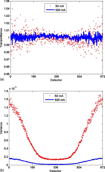
The following technique was used to determine the form of the bowtie filter profile, p(d). Because the x-ray path length through a patient is typically smaller in the periphery of the body relative to its center, bowtie filters shape the intensity of the incident x-ray beam into a nonuniform flux across the fan beam to minimize dose to the patient³² and to obtain equal signal over all rays exiting the patient. Specific bowtie profiles are provided for scans of particular parts of the anatomy, e.g., head bowties have a narrower fan beam of flux compared to body filters. The result of the bowtie filter is a reduced flux in the outer region of the fan beam. If there is no attenuating object present, this creates higher noise levels in periphery regions relative to the isocenter. CT scanners are calibrated to produce data for filtered backprojection that will have a uniform mean attenuation of zero for air; so a scan of an empty gantry produces a sinogram with essentially constant mean value (zero) for attenuation (or unity for transmittance) for each detector across the fan beam; this profile for one detector row is shown in Fig. 1a. However, due to the variation in flux level across the fan beam, variance across the field of view of detectors is not constant [Fig. 1b]. [Note: Engel et al.,³³ recently demonstrated that the presence of objects adds measureable scatter signal (up to 10% of primary flux) in direct exposure regions. This effect was not analyzed in this study.] As is shown in Appendix A1, measuring the noise in a detrended transmission signal as a function of detector position d provides an estimate of the relative transmission of the bowtie filter, p(d).

Figure 1.

The effect of bowtie filter on signal statistics. (a) Plot of mean transmittance signal as a function of detector position for air scans at 50 (points) and 500 mA s (line) in a 16-row scanner, with mean transmittance of $\overline{T_d\left(50\mathrm{mA}\right)}=1.0002\pm 0.0019$ and $\overline{T_d\left(500\mathrm{mA}\right)}=1.0001\pm 0.0009$ over 2000 gantry steps. (b) Plot of the variance of transmission signal for the same two scans. While the means are similar and relatively constant, the variance is non-uniform, being greatest in the low-flux periphery areas, and its magnitude is inversely proportional to the current.

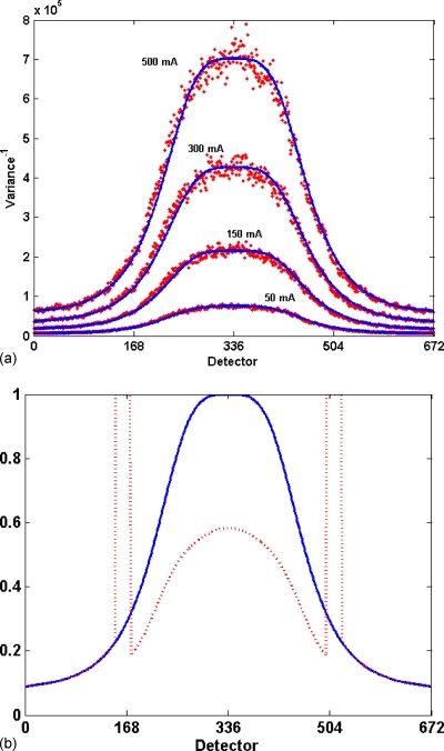
The variance of the cross-gradient (Appendix A2) at each detector position was computed for multiple gantry positions [e.g., 1400 (for head protocol) or 2500 (for body protocol) gantry steps], and the profile of this variance versus detector index was fit to an eighth-order polynomial function; the normalized inverse of this fit serves as the bowtie filter transmission profile, p(d). The accuracy of the profile was estimated by computing the root-mean-square (rms) of the relative error between the measured variance and the inverse of the fitted profile,$E_{\mathrm{rms}}=\sqrt{1∕N_d\sum _{d=1}^{N_d}{({\sigma }_T^2\left(d\right)-(1∕p\left(d\right)\lambda \left(d\right))∕(1∕\left(p\left(d\right)\lambda \right(d\left)\right)\left)\right))}^2}=\sqrt{\sum _{d=1}^{N_d}{[1-p\left(d\right)\lambda {\sigma }_T^2\left(d\right)]}^2∕N_d}.$As shown in Appendix A4, E_rms must be corrected for bias due to stochastic fluctuations of the measurements. (For comparing measurements to the profile, there is no noise contribution to bias from the profile polynomial.)

Incident flux

The following technique was developed to measure the scaling factor relating the tube current to the x-ray quantum flux. Solving Eq. 7 for the scaling factor K gives

$$K=\frac{Q_0\left(\mathrm{g}\right)}{cmA\left(g\right)s}.$$ (10)

As shown in the Appendix A1, Q₀(g) is inversely proportional to the variance of the transmittance signal ${\sigma }_T^2(d,g)$ and the bowtie filter profile, p(d). Therefore, Q₀(g) can be estimated by averaging the detrended noise ${\sigma }_{\mathrm{CG}}^2(d,g)={\sigma }_T^2(d,g)∕4$ given in Appendix A4 over all detectors for an air scan $[\overline{T}(d,g)=1]$,

$$Q_0\left(g\right)=\frac{1}{N_d}\sum _{d=1}^{N_d}\frac{1}{4p\left(d\right){\sigma }_{\mathrm{CG}}^2(d,g)}.$$ (11)

K can be estimated by averaging Eq. 10 over all gantries

$$\overline{K}=\frac{1}{N_g}\sum _{g=1}^{N_g}\left[\frac{\overline{Q_0\left(g\right)}}{cmA\left(g\right)s}\right].$$ (12)

To determine the intrascanner variability of K, air scan measurements were performed at four different current levels (50, 150, 300, 500 effective mAs), and a mean and standard deviation for K was calculated. To estimate interscanner variability, means of K for three different scanners in the BJC Hospital complex were calculated and a standard deviation computed.

A variation of this technique can be useful in determining the flux level in any clinical scan, including those using tube-current modulation, even if the instantaneous tube current value is not available. Most scans have sinogram data that include some regions outside the patient with direct exposure (air only) measurements. These air regions in the sinogram data can be segmented, e.g., by thresholding for transmittances greater than 0.99, to collect samples with direct exposures. The variance of cross gradient of the signal from the selected segmented regions normalized by the bowtie filter profile represents the flux (Q₀) of the scan given by Eq. 11. This method can thus be used to measure tube-current modulation or to validate tube-current parameters extracted from data file headers.

Electronic system noise

Electronic system noise is several orders of magnitude smaller than the quantum noise present in the direct beam, and hence, only becomes appreciable in the presence of a highly attenuating object. A method for measuring this component is described by Whiting et al.¹⁸ and involves scanning a precisely aligned cylinder object; fitting the sinogram profile signals to a parameterized model; and obtaining the signal statistics from fluctuations about this mean “reference truth” model. From such measurements, variance can be plotted as a function of signal magnitude, with the intercept of the fitted linear equation being equal to the system noise.

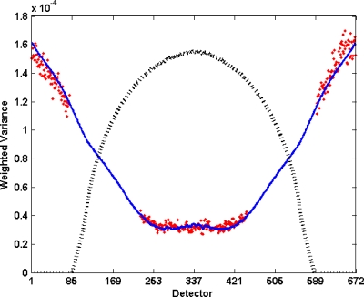
A less complicated and more convenient estimate of system noise was obtained by scanning a highly attenuating cylinder and assuming that the sinogram attenuation profile of the cylinder was stationary during one rotation. (A cylinder could be centered to within 3–4 mm of the isocenter, which leads to systematic intensity modulation in the profile near the edges of the cylinder that would distort estimates of stochastic noise. The magnitude of this systematic modulation as a function of position in the cylinder profile was estimated by the methods of Whiting and Muka³⁴ or Earl.³⁰ Data were analyzed only in regions where stochastic noise comprised more than 98% of the signal energy, which was typically the central 200–300 detectors.) The mean and variance of the transmittance signal [T(d,g)=e^−A(d,g)] were calculated for each detector location. Rewriting Eqs. 1, 2 in terms of the transmittance gave the measured variance in terms of the measured mean, ${\sigma }_S^2=\kappa \overline{S}+N_0$, with two adjustable parameters, κ and N₀. These parameters were determined by using a nonlinear Nelder–Mead simplex optimization (MATLAB, fminsearch) to minimize the mean-square relative error between the measured and modeled variance, averaged over all detectors (see Fig. 2). Edges of the cylinder, which contain high variance due to positioning sensitivity caused by large edge gradients, were excluded. This resulted in an estimate for the incident flux scaling factor (κ) and system noise (N₀).

Figure 2.

Plot of transmittance variance divided by mean transmittance as a function of detector position for scan of a 35.4 cm cylinder for 50 mA s. For uniform flux (no bowtie) with no additive system noise, this would be expected to be a constant, but the bowtie filter and system noise cause excess variance. Points represent the measurement and the solid line represents the noise model of Eqs. 1, 2, with parameters (K=3242 and N₀=38) selected to minimize the square of the relative error. The dotted line corresponds to cylinder profile (not to scale) as a function of detector position.

Influence of model components

The effect of the bowtie filter and background noise on image properties was observed by producing simulated images with different combinations of these components enabled, such as including or excluding the bowtie filter in the simulation of low-dose cylinder scan from a high-dose cylinder scan. Noise statistics (means, standard deviations) were measured in regions of interest (ROI) in the images, and comparisons were made between them. In addition, visual inspection of simulated clinical images, with and without the components, revealed the visual impact they had on image features.

Simulation validation

To validate the dose-reduction simulation, statistics from both the sinogram and image domain were compared for low-dose simulations (obtained from high-dose scans) and actual measured low-dose scans. Observer studies were also conducted to assure that simulated images appeared realistic.

Quantitative analysis in sinogram domain

Scans of a 35.4-cm diameter PMMA cylinder were obtained with four current levels (50, 150, 300, and 500 effective mAs), using 120 kVp, 16×0.75 mm collimation, pitch equal 1.0, and a 0.5 s rotation time. Sinogram data at the higher effective mAs were used as the basis for a lower-dose simulated sinogram. In the sinogram data domain, the variance was calculated for all detectors over 3000 gantry steps, as was the rms relative error between the original and simulated scans $[\mathrm{rmsRE}=\sqrt{{\left(\right(\text{original}-\text{simulated})∕\text{simulated})}^2}]$. As shown in Appendix A4, this rms relative error has a bias due to the stochastic noise in the variance measurements; a correction was applied to the rms relative error by subtraction of the computed bias from the mean-square relative error. The magnitude of this effect was estimated by performing two simulations with the same data and same parameters—the magnitude of this rms relative error was 7.29%, in agreement with a calculated bias of 8.3%.

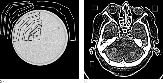
Quantitative analysis in image domain

In the image domain, multiple ROIs were selected, and the means and standard deviations were calculated for corresponding locations in both original and simulated slices. For cylinder phantom scans, eleven slices were selected from images and ten ROIs were chosen in each slice [Fig. 3a], resulting in a total of 110 ROIs for comparison. Simulated lower-dose scans were prepared from higher dose scans: three sets for 50 mAs (from 150, 300, 500), two sets for 150 mAs (from 300 and 500), and one set for 300 mAs (from 500 mAs ). This gave a total of six sets of simulated ROIs to be compared with three sets of original ROIs, for a total of 660 comparisons.

Figure 3.

Images of cylinder and cadaver head, showing selected ROI. Statistics for each ROI were collected and analyzed. Plot of image-domain noise shown in Fig. 12 to determine accuracy of simulations.

For cadaver-head scans, 31 slices were selected, with seven ROIs in each slice [Fig. 3b], including areas of exterior air and interior areas of bone and soft tissue, for a total of 217 ROIs per current level. Again, four current levels were acquired, with three original measurements and six simulated measurements from the higher dose scans, for a total of 1302 ROIs for comparison. Between scans, the cadaver head changed orientation slightly, so that reconstructed images could not be exactly aligned and the difference image contained major artifacts. Therefore, the means of ROI statistics were calculated for exterior and interior regions of each scan, and the relative error between means was reported, rather than computing the rmsRE on a pixel-by-pixel basis.

The rmsRE between the standard deviations of the ROIs was reported as a measure of accuracy. Note that, due to the stochastic noise of individual scans, even with a perfect simulation model there would be a finite rms relative error between any two scans. The analysis in Appendix A4 provides an estimate of this variance floor as a function of individual measurement variances, and a correction was applied (subtracting a variance floor from the measured variance) to remove this bias from the reported results.

Image domain observer study

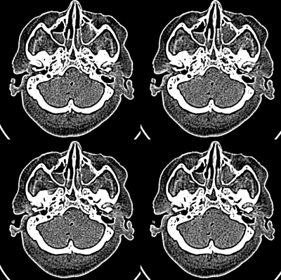
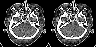
In addition to quantitative testing of simulation results, it is important that observer studies be performed to insure that simulations appear realistic to radiologists. Images of a cadaver head were used to conduct a four-alternative forced-choice observer study³⁵ (4AFC) for the ability to distinguish simulated from original images. Scans of the cadaver head were performed at four current levels (50, 150, 300, and 500 mAs ) (Fig. 4). The raw data from the higher current levels were used for a simulation of images at the lowest current level of 50 mAs , providing images from four source currents (150, 300 mAs , and two instances from the 500 mAs scan). Six original and 12 simulated image slice positions (out of 31 reconstructed slices available) were selected for the observer experiment. Sets of four images were created, with a random selection of one original and three simulated. The four images were randomly placed in the four-up matrix. The observer was instructed to select one image (the “original”) that had different noise characteristics from the other three. Forty sets of four images (total of 160 images) were displayed one set at a time, and an attendant manually recorded the position of the image choice selected as the original by the observer. The relative frequency with which an observer picked each image from the set was calculated, with the expectation that a 25% frequency would indicate random selection (no difference between the original and simulated images). Because the selection is a binomial process, the responses are not expected to be normally distributed. (Normal curves were fit to the relative frequencies and the normality of the data distributions were tested with Shapiro–Wilk W tests. If data were not normally distributed, the arcsine transformation was performed on the relative frequencies,³⁶ and the normality of the transformed data was tested.) The arcsine-transformed data were entered into a repeated measures analysis of variance. Statistical analyses were performed with JMP Statistical Software (SAS Institute, Inc., Cary, NC).

Figure 4.

Image of four-up cadaver head used in 4AFC study. Upper left simulated 150–50 mAs ; upper right original 50 mAs , lower left simulated 300–50 mAs , and lower right simulated 500–50 mAs .

Six radiologists with a mean clinical experience of 10.7 years (range: 7–17 years) participated in the experiment. Before the study, they received the following orientation in distinguishing between the original and simulated images. Two image sets were provided. Each set consisting of the original images at all four dose levels presented next to each other, as well as samples of lower-dose simulated images generated from the three higher-dose raw data scans (same slice location as shown in first step) presented next to the corresponding original image (total of 12 sample dose levels). The observers were allowed to view all samples with no time limit and an attendant was present to answer any questions.

Just noticeable difference

To establish guidelines for the accuracy required in noise simulation, experiments were performed to determine the amount of difference between image noise levels that could be discerned by observers. This was measured as the JND,¹⁹ which is defined as the point at which an observer operates midway between random guessing and perfect certainty. A 2AFC experiment was conducted, for which the JND performance level is 75%{=[random guessing(50%)+perfect certainty(100%)]∕2}. Images were prepared from a 500-mAs cadaver head scan, containing 151 slices; all the image slices had nominally comparable noise levels. A reference low-dose simulated noise level was set at 50 mA s and compared with five higher-dose levels, with dose differing by 10% (55 mAs ), 20% (60 mAs ), 30% (80 mAs ), 40% (90 mAs ), and 100% (100 mAs ). For each of the above noise levels, 40 slices were randomly selected from the 151 slices available, and paired simulated images at the two different dose levels were displayed next to each other, with a random order for the position of the lower dose image (Fig. 5). Observers were asked to select the image in the pair that had lower noise, which was recorded by an attendant. The percentage of correct choices was calculated for each noise level; no detectable difference in noise levels is expected to result in a 50% correct rate, while a large difference in noise levels would give a 100% correct rate. Results of percent correct were plotted versus dose level for the group average and for each individual to determine the dose level at which the JND rate was 75%.

Figure 5.

Presentation image for two cadaver head slices used in JND study (simulated images were prepared from a 500-mAs cadaver head scan). Image on the right is simulated at 50 mAs current level, left image is simulated at 60 mAs current level, corresponding to 20% difference in dose level and a 10% difference in standard deviation.

Five radiologists with a mean clinical experience of 11.4 years (range: 7–17 years) participated in the study. Each received an orientation session to the observer task, consisting of viewing one image slice that was simulated with varying noise levels, with the four different noise levels presented side-by-side for inspection.

RESULTS

Simulation parameters

Statistical properties of sinogram data

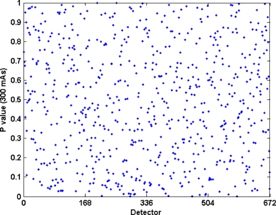
The χ² tests supported the hypothesis that sinogram data has Gaussian distributions. In the air scan experiments, the computed p values for all individual detector channels (N_det=10 752=16^*672) appeared uniformly distributed over the region from 0 to 1 (Fig. 6), and use of Fisher’s method analysis indicated that they satisfied the Gaussian hypothesis at the 0.05 significance level, with p_X values of 0.298, 0.475, 0.130, and 0.119 for 500, 300, 150, and 50 mAs , respectively. Similar results were obtained for central-region detectors (N_det=5616=351^*16) of the 35.4-cm-diameter cylinder phantom scans, for the same four current levels: for the χ² tests, Fisher’s method indicated agreement with p_X values of 0.612, 0.821, 0.722, and 0.401 for 500, 300, 150, and 50 mAs , respectively. Combining the p_X values from all objects and current levels by Fisher’s method gives a p value=0.54, indicating that the detector measurements were normally distributed.

Figure 6.

Plot of p values computed from chi-square test for one row of air scan data at 300 effective mAs. Minimum measured p value is 5.2728^*10⁻⁴. Fisher’s method analysis indicated the p values are uniformly distributed with a p_X value of 0.54.

Bowtie filter profile

Bowtie filter profiles were calculated from variance measurements for an open gantry scan [Fig. 7b]; a plot of the fitted polynomial for the body bowtie filter is shown in Fig. 7a. In this case, the unbiased rmsRE between the polynomial fit and the measured inverse variance, averaged over all detectors, was less than 1%, indicating an excellent estimation of the flux profile. (From the discussion in Appendix A3, the noise variance in the measured signal generates a bias floor in rmsRE estimated to be about 3%, so unbiased estimate of agreement was better than 1%.) The rmsRE among the bowtie profiles obtained with four different currents was 1.3%±0.9% (standard deviation), with a maximum individual difference of less than 2.8%. Note that the ratio of the flux at the isocenter compared with the edge of the fan beam varied by a factor of 8.

Figure 7.

(a) Plot of reciprocal of variance (proportional to incident flux on object) determined by air scan (points), with its corresponding fitted curve (line). (b) Bowtie filter profile obtained by normalizing fitted variance curve, shown for body (solid) and head (dotted) protocols.

Incident flux

To determine the intrascanner variation of the scaling factor K, a series of controlled scans at four different current settings on one scanner resulted in a mean value of 3288 with a standard deviation of 4.5% characterizing the scan-to-scan fluctuations. From the relationship Q=KcmAs, this K implies a range of fluxes at the isocenter between 69 000 and 674 000 from the minimum (50 mA, 0.5 s rotation, 0.75 mm collimation) to maximum (500 mA, 0.5 s rotation, 0.75 mm collimation) currents, respectively. To measure the interscanner variation, K was also computed from air sections in seventeen clinical scans for three different scanners, which resulted in individual standard deviations of 4.2%, 4.4%, and 4.4%, indicative of the intrascanner variability. Computing the interscanner variation in K between the three scanners resulted in a standard deviation of 14.5%, indicating that noise calibration of individual scanners is required to achieve simulation noise accuracies of approximately 5%.

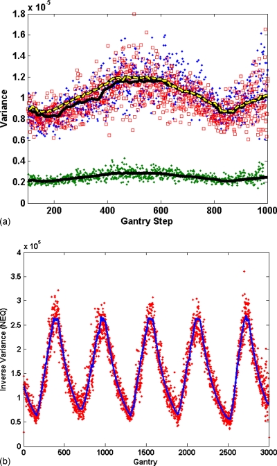
The effect of tube-current modulation on flux was demonstrated by prediction of the variance of the air region of the sinogram for a skull object, shown in Fig. 8a. The stochastic bias in the rmsRE was predicted (Appendix A4) to be 14.9% for tube current on and 15.0% for tube current off. The measured rmsRE agreed to within 1.3%±0.4% for tube current on and 1.5%±0.7% for tube current off. A similar measurement was performed for a clinical patient scan, where the rmsRE between predicted and measured K was found to be 2.2% [Fig. 8b].

Figure 8.

Inverse of measured variance in air region outside objects scanned with tube-current modulation enabled. Line represents scaled tube current, open markers are the simulated and solid markers are real scans. (a) Skull scan with tube modulation on for 250 mAs (lower) and both simulated and original 50 mAs (upper), (b) a patient body scan.

Electronic system noise

System noise N₀ was calculated from fits of the variance model [Eqs. 1, 2] to measured scans of a highly attenuating cylinder. N₀ was found to have a linear dependence on increasing tube current, N₀=0.7841^*cmAs+22.46. (Such dependence might occur if the analog electronics chain contained an adjustable gain stage, selected for particular mA settings in a protocol, to scale the signal range, followed by a fixed noise source.) N₀ varies from 40 to 200 NEQ over the range of currents, indicating that system noise contributes less than 0.1% to the total variance in the direct beam and only becomes appreciable for maximum log attenuations greater than 10, such as for large patients (diameter >40 cm) or in the presence of metal prostheses.

Evaluation of simulation model components

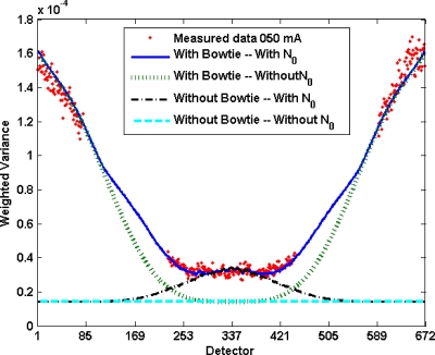
Analyzing the variance in a cylinder scan reveals the magnitude of contribution of various model components. A plot of variance versus detector position (Fig. 9) shows that the bowtie profile is necessary to match noise levels away from the isocenter, while including N₀ is necessary to generate accurate noise in regions of high attenuation. Without these components, large errors were seen, e.g., 50% at the isocenter and 90% in the periphery.

Figure 9.

The effect of various components on noise. Conditions are the same as Fig. 2, with solid line representing complete noise model fit to experimental data (dots). The dotted lines present the model with and without inclusion of bowtie filter profile and system noise. For uniform flux with no additive system noise, the model profile would be a constant for all detectors. The bowtie profile contributes rising noise away from the isocenter, while system noise increases noise primarily in the center of the cylinder.

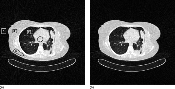
The visual effects of noise components in clinical images can be seen in Fig. 10, where it is observed that in a thoracic scan it is not possible to match noise in the center and edges of the chest (leading to errors in noise higher than 44%) without including the bowtie profile and system noise.

Figure 10.

Simulated images created by including a bowtie filter (left) and without one (right), with noise levels matched in the center of the image. Note appearance of noise levels in indicated regions. The percentage difference between two simulations is 1.8% in ROI No. 1 (center), 2.8% in ROI No. 2 (lung), 50.9% in ROI No. 3 (tissue-periphery), 44.6% in ROI No. 4 (tissue-periphery), and 28.3% ROI No. 5 (air-periphery).

Simulation validation

Quantitative analysis in sinogram domain

In the cylinder scans, the variance as a function of a detector position was measured for original and simulated scans; the rmsRE between the two was computed, and it was corrected for the bias of stochastic noise. The rmsRE was 5.2%±1.0% (standard deviation) for 50 mAs simulations, 6.5%±3.1% for 150 mAs simulations, and 5.8% for the 300 mAs simulation. The overall rmsRE was 5.6%±1.6%. The maximum rmsRE was less than 9% for all individual cases.

Quantitative analysis in image domain

Over the 660 ROIs in the cylinder phantom images that were compared, the rmsRE between the standard deviation of the simulated and original images was 5.7%±2.1% (three sets of 50 mAs simulations, 330 ROI), 4.2%±1.2% (two sets of 150 mAs simulations, 220 ROI), and 2.4%±0.6% (one set of 300 mAs simulation, 110 ROI), with an overall mean rmsRE of 4.1%±1.6% and a maximum individual error of 9.3% (only for one of the ROIs at 50 mAs ). The rmsRE averages for the 1302 ROIs of cadaver head images were 4.7% (50 mAs ), 0.5% (150 mAs ), and 5.3% (300 mAs ) for interior regions, and 2.8% (50 mAs ), 1.2% (150 mAs ), and 0.9% (300 mAs ) for exterior regions (see Table 1).

Table 1.

Comparison of simulation accuracy for cadaver head shown in Fig. 3b. ROI standard deviations and relative errors of tissue and air regions are listed. Original measurements are bold.

		50	150	300	500
Tissue	Original or simulated 50 mAs	35.8±4.6	37.1±4.5 (−3.77%)	37.6±4.4 (−5.16%)	37.6±4.0 (−5.03%)
	Original or simulated 150 mAs	NA	21.1±2.7	21.2±2.6 (−0.61%)	21.1±2.7 (−0.36%)
	Original or simulated 300 mAs	NA	NA	15.8±2.1	15.0±1.8 (5.28%)
Air	Original or simulated 50 mAs	19.2±1.9	19.9±2 (−2.48%)	19.5±1.9 (−1.73%)	19.6±2.1 (−3.77%)
	Original or simulated 150 mAs	NA	12.9±1.7	13.0±1.6 (−1.10%)	12.7±1.5 (1.32%)
	Original or simulated 300 mAs	NA	NA	10.5±1.3	10.4±1.2 (0.88%)

Image domain observer studies

The 4AFC test data were analyzed to test the equivalence of simulated and real images in observer viewing. The distributions of frequencies for image selections were non-normal (p<0.05, Table 2). After arcsine transformation, however, the data were normally distributed (p>0.05) and differences were tested for statistical significance with a repeated measures analysis of variance. Individual observers varied in their abilities of selecting original images, ranging from a frequency of 17.5% to 40% (Table 2). There was no significant difference between the selection of simulated or original images, indicating that the selection was random to within experimental error (p=0.86).

Table 2.

4AFC study results. 40 sets of four-up images (one original, and three simulated selected from four source currents) were presented as shown in Fig. 4. Percentage of selection for each image source indicates that the simulations are indistinguishable from originals, with all selections being effectively random (25%).

	Simulated 150–50 mAs	Simulated 300–50 mAs	Simulated 500–50 mAs	Simulated 500–50 mAs	Original 50 mAs
# images presented	22	30	34	34	40
Observer 1	2 (0.09)a	6 (0.20)	11 (0.32)	5 (0.15)	16 (0.40)
Observer 2	7 (0.32)	3 (0.10)	14 (0.41)	9 (0.26)	7 (0.18)
Observer 3	3 (0.14)	8 (0.27)	4 (0.12)	16 (0.47)	9 (0.23)
Observer 4	5 (0.23)	16 (0.53)	5 (0.15)	7 (0.21)	7 (0.18)
Observer 5	4 (0.18)	4(0.13)	13 (0.38)	10 (0.29)	9 (0.23)
Observer 6	8 (0.36)	4 (0.13)	12 (0.35)	4 (0.12)	12 (0.30)
Mean probability	0.22±0.1b	0.23±0.16	0.29±0.13	0.25±0.13	0.25±0.09

^aNumber of picks and relative frequency [for example, observer 1 picked “Simulated 150–50 mAs ” image 9% (2 of 22) of the time].

^bMeans±standard deviations.

Just noticeable difference

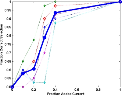
Data from the 2AFC test were analyzed to determine the sensitivity of observers to changes in noise level. The frequency for correctly identifying the lower noise image is plotted versus fractional change in current level for individual observers and the mean of all observers. The JND point (75%) corresponds to approximately a 25% increase in current level, as seen in Fig. 11. Individual observer’s JND varied between a 20% and 40% increase in current level. Note that a fractional increase in current level gives rise to a square-root increase in σ_HU, e.g., 25% more current results in a 12% decrease in σ_HU. Results reported in this article are consistent with observer studies involving photographic images,³⁷ where the JND for an “average” photograph was found to correspond to a 15% increase in rms granularity. This JND serves as a target benchmark for accuracy levels in simulations, i.e., images with noise matched to within this tolerance will appear equivalent.

Figure 11.

Plot of fraction of low-dose images correctly identified vs the amount of additional current in one of the image pair. Data for five individual observers are presented with dotted lines, and solid line represent mean of all observers. The JND point (75% correct) for the mean of all observers is approximately 25% added current, while the JNDs for individual observers vary between 20% and 40% added current.

DISCUSSION

These experiments demonstrated that tube-current reduction simulation can be a useful tool for generating realistic images to be used in studying image quality as a function of radiation dose in CT examinations. Compared to simulations in the image domain,^{7, 38} methods based in the sinogram domain are straightforward and accurate. Detailed descriptions of the simulation methods were presented, including a general noise model; experimental techniques for determining parameters used in the simulation process; estimates of achievable accuracies in simulations; and criteria for simulation accuracy. To perform accurate noise synthesis, noise models must include varying fluxes, due to bowtie filters and tube-current modulation, and electronic noise sources; otherwise, fairly large errors (50%–90%) in simulated noise level can occur throughout an image. General experimental techniques, which could be extended to other scanner geometries, were presented for the convenience of determining model parameters, such as bowtie filter profile, flux level scaling, and system noise.

The statistical properties of sinogram measurements demonstrated the validity of using a Gaussian random noise generator for simulations, as a normal distribution was found to be appropriate for clinically relevant protocols. A recent report on sinogram statistics from the researchers at SUNY Stony Brook^{13, 39} presented a p value analysis of detector measurements. Their results indicated more disagreement from a normal population compared to the results presented here, which may be due to their differing experimental techniques: they computed statistics from repeated scans in the sinogram domain and used phantoms with complex anatomical structures. Also, it is difficult to interpret the statistical significance of the metrics that they reported (fraction of detectors with p values less than 0.05, which varied from 6% to 9% of the total number of detectors).

When simulating flux levels lower than the clinical conditions examined here, Gaussian noise properties ultimately become compound Poisson.¹⁸ Under those conditions, the signals should be converted into NEQ, and Poisson random number generators can be used.⁴⁰ The range of validity for a Gaussian process can be estimated using model parameters presented in this article, which were applied to an individual patient and scan protocol. Clinically, departure from Gaussian behavior might occur with large patients or in the presence of prosthetic metal implants. For instance, an abdomen scan of a patient with a 40 cm diameter might have maximum attenuations on the order of 8 natural logarithm units, which for a 500 mAs scan would give minimum flux counts on the order of 220 (=670 000^*e⁻⁸). In this case, a 10× dose reduction (to 22 NEQ) could be accurately simulated with Gaussian random noise generators.

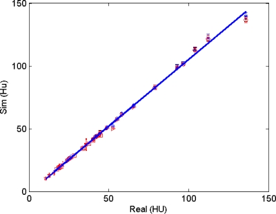
There are no reports of the comparison of simulated and real sinogram noise in the literature. In the image domain, several groups have reported on observer studies that compare real and simulated CT images, claiming very good results, but there is less information on quantitative testing. Mayo et al.¹² compared simulations in 27 patients at two current levels and found “no significant difference (minimum P>0.13)” in the noise levels measured in aortas, although not enough information was provided to determine noise characteristics. Frush et al.¹¹ measured real and simulated noise in a 25 cm phantom at four current levels, reporting no statistically significant difference, with agreement on the order of a few percent. Mackenzie, et al.⁴¹ recently reported measurements with a correlation coefficient between real and simulated noise of 0.99, although their graphs of data seemed to show noise discrepancies on the order of 10%. (Note that if the simulated versus real measurements presented in this article are plotted against each other, Fig. 12, a very high correlation coefficient is found (r=0.999), even though the rmsRE analysis indicates a 5% mismatch.)

Figure 12.

Plot of real vs simulated image-domain noise (standard deviation in HU) for cadaver head (31 slices as shown in Fig. 3) and cylinder phantom (11 slices as shown in Fig. 4), with a total of more than 2000 ROI. The correlation factor of all data points is r=0.999 28; with r=0.998 49 for cylinder measurements, and r=0.9988 for cadaver head, respectively.

The techniques described produced accuracies in noise simulation on the order of ∼5% for individual scanners. (Variations in parameters were on the order of 15% between different machines, indicating that parameter calibration for individual scanners must be done.) Measurements showed the matching of noise statistics in the sinogram domain between original and simulated data to within 5.6%, which propagates into the image domain. More importantly, observer studies indicate that the simulated images are realistic, with no detectable difference between simulated and original images. (Individuals participating in the observer studies commented that it was very difficult to choose between original and simulated images.) The JND studies indicate that observers can reliably detect changes in noise levels corresponding to 25% changes in tube current. This level of noise sensitivity is consistent with studies performed with human observers on photographic film, indicating that accuracies in simulation on the order of ∼10% would result in images that could not be reliably differentiated from original images.

Finally, it should be noted that the methods presented here are intended to simulate techniques that lower dose by decreasing the tube current, without changing other protocol parameters that affect patient dose, such as kVp, pitch, collimator size, or rotation time. All these parameters directly affect signal properties and have more complicated effects on images than just changing noise statistics. Also, note that for simulations of modest dose reductions, the magnitude of the added synthetic noise may be comparable or less than the existing original noise, which would cause the noise patterns in images created from one sinogram slice in multiple simulations not to be statistically independent. Thus, a single simulation image would represent realistic noise appearance but the use of multiple simulations from one base image in an experiment would require caution.

Also, the method requires access to sinogram data and knowledge of sinogram formats. Archiving of sinogram data is becoming more available on multirow detector CT scanners, and hence, availability of data files is more common. While reverse engineering of data structures is somewhat possible, documentation from vendors is preferred. (Such information was provided to our group under a research agreement with Siemens.) Several research groups, in addition to our own, have recently reported working with the raw data.^{10, 13, 14, 15, 16, 17} The techniques that have been presented in this article are general and useful on any scanner geometry. In addition to the results reported on 16-row scanner systems, comparable outcomes were obtained in experiments conducted on single-row helical scanners (Siemens Plus 4) and four-row scanners (Siemens Volume Zoom). For example, the older generation CT scanner (Siemens Plus 4) with much higher system noise was also accurately modeled with the developed techniques.

In summary, simulation tools, such as described in this article, have applications in several areas of improving CT acquisition. Because they can generate realistic low-dose clinical images, they can be used in determining the effects of image noise on observer performance for research, in obtaining the specification of protocols to achieve ALARA objectives, and in guiding the design of scanner system components. Simulation can be particularly valuable as a training device, allowing radiologists to explore the impact of lower doses and become comfortable with lower-dose protocols. In observer study experiments conducted for this research, it was noted that readers’ confidence in their ability to diagnose with low-dose images increased after spending time acclimating to images with lower dose levels. It would be prudent to conduct further research to take advantage of this capability.

APPENDIX A: CHARACTERIZATION OF NOISE

This research required the characterization of noise in CT images and raw data. Previously,¹⁸ methods were developed to measure statistics (i.e., probability density functions and higher order moments) of sinogram signal fluctuations, but such methods require careful control of experimental conditions and extensive analysis. In this research, for the simple evaluation of signal variance, more convenient and rapid methods were developed and are described. The basic ingredients of the approach are choice of the domain in which to represent the signals, mathematical operations on data to extract stochastic components, estimates of the accuracy of the variance measurements, and a method to quantify the similarity of two random processes.

Mean-variance relationships

Sinogram data can be represented in several different domains, and the relationship between the mean and variance are different in each.⁴² Data files consist of the natural logarithm of scaled measurements,A_m=log(S₀∕S_m), from which the fundamental linear measurement signal can be extracted S_linear=S₀e^−A_m. Here, S₀ is the mean signal in the absence of any object, known by calibration, and it is proportional to the x-ray flux λ, S₀=κλ. In the linear flux domain, substituting S₀ in Eq. 2 results in a variance that is proportional to the mean, ${\sigma }_{\text{linear}}^2=\kappa \overline{S_{\text{linear}}}$. (As shown by Whiting et al.,¹⁸ κ is a slowly varying function of the x-ray spectrum and changes on the order of +∕−3% across the range of clinical conditions. In this study, it is assumed to be a constant for all measurements.) For the varying incident flux across detector position d or gantry angle g, $[\overline{S}(d,g)=p\left(d\right)mA\left(g\right){\overline{S}}_0]$, and the variance remains linear with the mean, ${\sigma }_{\text{linear}}^2(d,g)=\kappa {\overline{S}}_{\text{linear}}(d,g)$.

It is often convenient to work with transmission ratios, i.e., the data are ratios of measured flux with an object present to the expected flux without the object. Transmittance values range from 0 to slightly larger than one (due to random excess fluctuations), with mean $\overline{T}=e^{-\overline{A}}={\overline{S}}_{\text{linear}}∕S_0$. In this case, the variance can be computed as ${\sigma }_T^2\approx {\mid \partial T∕\partial S_{\text{linear}}\mid }^2{\sigma }_{\text{linear}}^2={\mid 1∕S_0\mid }^2\kappa \overline{S_{\text{linear}}}=\kappa \overline{T}∕S_0=\overline{T}∕\lambda$; thus variance remains linear with the mean transmittance and becomes inversely proportional to the flux level. In particular, when $\overline{T}=1$, ${\sigma }_T^2$ is the inverse of the x-ray flux. In the case where the flux is varying, the mean transmittance remains independent of flux nonuniformity, while the transmittance variance is of the form ${\sigma }_T^2(d,g)=\kappa \overline{T(d,g)}∕S_{0}p\left(d\right)mA\left(g\right)=\overline{T(d,g)}∕\lambda p\left(d\right)mA\left(g\right)=\overline{T(d,g)}∕p\left(d\right)Q_0\left(g\right)$, showing an inverse dependence on the flux nonuniformities and providing a method to measure the bowtie profile p(d) when no object is present $(\overline{T}=1)$.

For linear reconstruction techniques (filtered backprojection), data are kept in log attenuation form. Here, the variance can be approximated as ${\sigma }_A^2\approx {\mid \partial A∕\partial S_{\text{linear}}\mid }^2{\sigma }_{\text{linear}}^2=\kappa \overline{S_{\text{linear}}}∕{\overline{S_{\text{linear}}}}^2=\kappa ∕S_0{e}^{\overline{-A}}=e^{\overline{A}}∕\lambda$, resulting in an exponential relationship between the mean and variance. Similarly, if the flux distribution varies as a function of detector position (due to bowtie filter) or gantry angle (due to tube current modulation), the mean is not affected and the variance is inversely related to variations of p(d) and mA(g): ${\sigma }_A^2=e^{\overline{A}}∕\lambda p\left(d\right)mA\left(g\right)$.

Finally, the behavior of signal variance can often be conveniently displayed by presenting “relative transmission” variance: ${\sigma }_v^2\equiv {\sigma }_T^2∕\overline{T}$. This is because for simple Poisson noise with uniform flux, the variance is proportional to the mean, so any deviation from this relationship (system noise, bowtie filter) shows up as an excess noise that is scaled relative to simple Poisson noise (see Fig. 9).

These relationships are helpful in experimentally establishing parameters, such as bowtie profiles or flux levels, for individual scanners.

Detrending

A fundamental challenge in measuring random signals is rejection of deterministic or systematic components, which typically contain low frequency energy.⁴³ For instance, in empty gantry scans, there are slow base line drifts due to x-ray tube fluctuations, or linear streaks due to nonuniform attenuators on the gantry shroud, either of which can contain appreciable signal energy. One way to suppress or detrend these errors is through differentiation of the signal.³¹ Differentiation removes low frequency and enhances high frequencies, so stochastic components can be extracted from measurements on smooth objects, such as air (a constant baseline) or the interior of symmetric cylinder phantoms. A cross-gradient operation CG was effective in this regard. This was implemented in MATLAB, using the gradient function [gradient(F_i)≡(F_i+1−F_i−1)∕2], as CG=∂²F∕∂g∂d=gradient[gradient(F^′)^′]. To relate the statistical properties of this detrended data to those of the original signals, note that ${\sigma }_{F_1-F_2}^2={\sigma }_{F_1}^2+{\sigma }_{F_2}^2$ and that the coefficient of 0.5 for both terms in the gradient is squared in the variance. Therefore, assuming that the variance of each term is approximately equal, ${\sigma }_{F_1-F_2}^2\approx ({\sigma }_F^2+{\sigma }_F^2)∕4={\sigma }_F^2∕2$, the cross gradient will have a computed variance that is one-fourth of the underlying original signal ${\sigma }_F^2=4{\sigma }_{\mathrm{CG}}^2$.

Precision of variance measurements

During the course of these experiments, results were frequently reported as variances of measurements or as the rmsRE between models and measurements. One question that arises is: “What is the expected precision of the reported quantity in a relative sense?” In other words, “What is the variance of the variance relative to the magnitude of the variance?” Saviane and Silver⁴⁴ derive an expression for the variance of the variance, which is unbiased for a “large” number of measurements n, as

$$\mathrm{Var}\left({\sigma }^2\right)=E\left[{\left({\sigma }^2\right)}^2\right]-{\left(E\left[{\sigma }^2\right]\right)}^2=\frac{{(n-1)}^2}{n^3}({\mu }_4-\frac{n-3}{n-1}{\mu }_2^2),$$

where μ_i is the ith central moment. They show that for Gaussian distributions, with μ₄=3σ⁴, this expression reverts to Var(σ²)=2σ⁴∕n for large n. Likewise, for Poisson distributions, μ₄=3λ²+λ and μ₂=λ, so Var(σ²)=(n−1)²∕n³{3λ²+λ−(n−3)∕(n−1)λ²}≈(2+1∕λ)∕nλ²=2σ⁴∕n. In both cases, the rms of the relative variance error becomes independent of the magnitude of the variance and depends on the number of measurements [Var(σ²)∕(σ²)²=2∕n]. In the case of measuring the variance for a detector over one revolution (e.g., N_g=1160), one would expect relative errors in the variance to be on the order of $\sqrt{2∕1160}=0.04$. Because the relative error of the variance is independent of the magnitude of the variance, one can use it to compare the noise properties of different detectors, even though each may have large differences in absolute variance due to the bowtie filter.

rms relative error

In this article, a rms relative error ($\mathrm{rmsRE}=\sqrt{{\sum }_i{[(m_i-s_i)∕m_i]}^2}$, where m and s refer to the measured or simulated data point i, is calculated for several quantitative analyses of the simulation process. This is very useful tool, but it is a biased estimator for the agreement of simulation with measurements, because even identical random processes will have nonzero rmsRE when repeated measurements are compared, due to the stochastic fluctuations at each point. The magnitude of this bias can be estimated with an approach similar to van Kempen and Vliet.⁴⁵ Performing a Taylor series expansion for the squared relative error $\widehat{R}={[(\widehat{s}-\widehat{m})∕\widehat{m}]}^2$ about its mean values

$$R(m,s)=R(\overline{m},\overline{s})+R_m(\overline{m},\overline{s})(\widehat{m}-\overline{m})+R_s(\overline{m},\overline{s})(\widehat{s}-\overline{s})\dots +\frac{1}{2}{R}_{mm}(\overline{m},\overline{s}){(\widehat{m}-\overline{m})}^2+\frac{1}{2}{R}_{ss}(\overline{m},\overline{s}){(\widehat{s}-\overline{s})}^2+R_{ms}(\overline{m},\overline{s})(\widehat{m}-\overline{m})(\widehat{s}-\overline{s})$$

and taking the expectation of the expansion gives $E\left[R(m,s)\right]=R(\overline{m},\overline{s})+R_{mm}(\overline{m},\overline{s}){\sigma }_m^2+R_{ss}(\overline{m},\overline{s}){\sigma }_s^2$, assuming no correlation between the measured and simulated noise, and no terms higher than second order in the expansion. This indicates that even in the case where the random processes are matched $(\overline{m}=\overline{s},{\sigma }_s^2={\sigma }_m^2)$, there will be a base line contribution given by $R_{mm}(\overline{m},\overline{s}){\sigma }_m^2+R_{ss}(\overline{m},\overline{s}){\sigma }_s^2=2{\sigma }_s^2∕{\overline{s}}^2+2{\sigma }_m^2(3{\overline{s}}^2∕{\overline{m}}^4-2\overline{s}∕{\overline{m}}^3)=4{\sigma }_s^2∕{\overline{s}}^2$. For example, in comparing the rmsRE for the variances of a simulated and measured sinogram, from Appendix A3, the variance of the variance is 2σ⁴∕N_g, so the base line error of the relative error would be 4(2σ⁴∕N_g)∕σ⁴=8∕1160, predicting an rms bias of 8.3%. The computed rmsRE can be corrected for bias by subtracting off this base line in quadrature.

References

- Kalender W. A., Computed Tomography: Fundamentals, System Technology, Image Quality, Applications, 2nd ed. (Publicis MCD Verlag, Munich, Germany, 2005). [Google Scholar]
- Brenner D. J. and Hall E. J., “Computed tomography—An increasing source of radiation exposure,” N. Engl. J. Med. 357(22), 2277–2284 (2007). [DOI] [PubMed] [Google Scholar]
- Frush D. P., Donnelly L. F., and Rosen N. S., “Computed tomography and radiation risks: what pediatric health care providers should know,” Pediatrics 112(4), 951–957 (2003). [DOI] [PubMed] [Google Scholar]
- Russell T. D. and Van Metter R. L., “Computer simulations demonstrating factors that influence the quality of radiographic images,” Radiology 173, 471 (1989). [Google Scholar]
- Saunders R. S. and Samei E., “A method for modifying the image quality parameters of digital radiographic images,” Med. Phys. 10.1118/1.1621870 30(11), 3006–3017 (2003). [DOI] [PubMed] [Google Scholar]
- Don S.et al. , “Preliminary validation of a new methodology for estimating dose reduction protocols in neonatal chest computed radiographs,” SPIE Medical Imaging 2006: Physics of Medical Imaging, 2006, Vol. 6142, pp. 61421W1–11.
- Britten A. J. et al. , “The addition of computer simulated noise to investigate radiation dose and image quality in images with spatial correlation of statistical noise: an example application to x-ray CT of the brain,” Br. J. Radiol. 77(916), 323–328 (2004). [DOI] [PubMed] [Google Scholar]
- Hanai K. et al. , “Computer-simulation technique for low dose computed tomographic screening,” J. Comput. Assist. Tomogr. 10.1097/01.rct.0000230011.16468.0e 30(6), 955–961 (2006). [DOI] [PubMed] [Google Scholar]
- van Gelder R. E. et al. , “CT colonography at different radiation dose levels: Feasibility of dose reduction,” Radiology 224(1), 25–33 (2002). [DOI] [PubMed] [Google Scholar]
- Sennst D. A. et al. , “An extensible software-based platform for reconstruction and evaluation of CT images,” Radiographics 24(2), 601–613 (2004). [DOI] [PubMed] [Google Scholar]
- Frush D. P. et al. , “Computer-simulated radiation dose reduction for abdominal multidetector CT of pediatric patients,” AJR, Am. J. Roentgenol. 179(5), 1107–1113 (2002). [DOI] [PubMed] [Google Scholar]
- Mayo J. R. et al. , “Simulated dose reduction in conventional chest CT: Validation study,” Radiology 202(2), 453–457 (1997). [DOI] [PubMed] [Google Scholar]
- Wang J. et al. , “An experimental study on the noise properties of x-ray CT sinogram data in Radon space,” Phys. Med. Biol. 10.1088/0031-9155/53/12/018 53(12), 3327–3341 (2008). [DOI] [PMC free article] [PubMed] [Google Scholar]
- King M.et al. , “Chord-based image reconstruction from clinical projection data,” SPIE Medical Imaging 2008: Physics of Medical Imaging, 2008, Vol. 6913, p. 69132G.
- Kudo H. et al. , “Tiny a priori knowledge solves the interior problem in computed tomography,” Phys. Med. Biol. 10.1088/0031-9155/53/9/001 53(9), 2207–2231 (2008). [DOI] [PubMed] [Google Scholar]
- Wunderlich A. and Noo F., “Image covariance and lesion detectability in direct fan-beam x-ray computed tomography,” Phys. Med. Biol. 10.1088/0031-9155/53/10/002 53(10), 2471–2493 (2008). [DOI] [PMC free article] [PubMed] [Google Scholar]
- Yu L.et al. , “Sinogram smoothing with bilateral filtering for low-dose CT,” Medical Imaging 2008: Physics of Medical Imaging, 2008, Vol. 6913, p. 691329.
- Whiting B. R. et al. , “Properties of preprocessed sinogram data in x-ray computed tomography,” Med. Phys. 10.1118/1.2230762 33(9), 3290–3303 (2006). [DOI] [PubMed] [Google Scholar]
- Linschoten M. R. et al. , “Fast and accurate measurement of taste and smell thresholds using a maximum-likelihood adaptive staircase procedure,” Percept. Psychophys. 63(8), 1330–1347 (2001). [DOI] [PubMed] [Google Scholar]
- Massoumzadeh P., Earl O. A., and Whiting B. R., “Noise simulation in x-ray CT,” SPIE Medical Imaging 2005: The Physics of Medical Imaging, 2005, Vol. 5745, pp. 898–909.
- Wang J. et al. , “Penalized weighted least-squares approach to sinogram noise reduction and image reconstruction for low-dose x-ray computed tomography,” IEEE Trans. Med. Imaging 10.1109/TMI.2006.882141 25(10), 1272–1283 (2006). [DOI] [PMC free article] [PubMed] [Google Scholar]
- Dainty J. C. and Shaw R., Image Science (Academic, London, 1974), pp. 171–182. [Google Scholar]
- Barrett H. H., and Myer K. J., Foundations of Image Science (Wiley-Interscience, Hoboken, NJ, 2004), p. 407. [Google Scholar]
- Rasband W. S., ImageJ 1997–2006, U.S. National Institutes of Health, Bethesda, Maryland.
- Kalender W. A. et al. , “Dose reduction in CT by on-line tube current control: Principles and validation on phantoms and cadavers,” Eur. Radiol. 9(2), 323–328 (1999). [DOI] [PubMed] [Google Scholar]
- Press W. H.et al. , Numerical Recipes in C, 2nd ed. (Cambridge University Press, New York, 1994), pp 620–623. [Google Scholar]
- Press W. H.et al. , Numerical Recipes in C, 2nd ed. (Cambridge University Press, New York, 1994), pp. 660–661. [Google Scholar]
- Riffenburgh R., Statistics in Medicine (Academic, San Diego, 1990), p. 318. [Google Scholar]
- Fisher R. A., “Combining independent tests of significance,” Am. Stat. 2(5), 30 (1948). [Google Scholar]
- Earl O. A., “Modeling noise in x-ray CT,” Electrical Engineering (Washington University, St Louis, MO, 2004). [Google Scholar]
- Rank K., Lendl M., and Unbehauen R., “Estimation of image noise variance,” IEE Proceedings-Vision Image and Signal Processing 146(2), 80–84 (1999). [Google Scholar]
- Toth T., Ge Z., and Daly M. P., “The influence of patient centering on CT dose and image noise,” Med. Phys. 10.1118/1.2748113 34(7), 3093–3101 (2007). [DOI] [PubMed] [Google Scholar]
- Engel K. J.et al. , “Spectral analysis of scattered radiation in CT,” SPIE Physics of Medical Imaging, 2008, Vol. 6913, p. 69131R.
- Whiting B. R. and Muka E., “Image quantization: statistics and modeling,” SPIE Physics of Medical Imaging Conference 1998, 1998, Vol. 3336, pp. 260–271.
- Burgess A. E., “Comparison of receiver operating characteristic and forced choice observer performance measurement methods,” Med. Phys. 10.1118/1.597576 22(5), 643–655 (1995). [DOI] [PubMed] [Google Scholar]
- Portney L. G. and Watkins M. P., Foundations of Clinical Research: Applications to Practice (Appleton & Lange, Norwalk, CT, 1993), p. 670. [Google Scholar]
- Zwick D. and Brothers D. L., “RMS granularity: Determination of just-noticeable differences,” Photograph. Sci. Eng. 19(4), 235–238 (1975). [Google Scholar]
- Li X.et al. , “Towards assessing the diagnostic influence of dose reduction in pediatric CT: A study based on simulated lung nodules,” SPIE Physics of Medical Imaging, 2008, Vol. 6913, p. 69131L.
- Wang J.et al. , “Noise properties of low-dose x-ray CT sinogram data in radon space,” SPIE Physics of Medical Imaging, 2008, Vol. 6913, p. 69131M. [DOI] [PMC free article] [PubMed]
- Lasio G. M., Whiting B. R., and Williamson J. F., “Statistical reconstruction for x-ray computed tomography using energy-integrating detectors,” Phys. Med. Biol. 10.1088/0031-9155/52/8/014 52(8), 2247–2266 (2007). [DOI] [PubMed] [Google Scholar]
- MacKenzie J. D. et al. , “Reduced-dose CT: Effect on reader evaluation in detection of pulmonary embolism,” AJR, Am. J. Roentgenol. 189(6), 1371–1379 (2007). [DOI] [PubMed] [Google Scholar]
- Beenakker C. and Schonenberger C., “Quantum shot noise,” Phys. Today 56(5), 37–42 (2003). [Google Scholar]
- Flynn M. J. and Samei E., “Experimental comparison of noise and resolution for 2k and 4k storage phosphor radiography systems,” Med. Phys. 10.1118/1.598656 26(8), 1612–1623 (1999). [DOI] [PubMed] [Google Scholar]
- Saviane C. and Silver R. A., “Estimation of the variance of the variance: implications for multiple-probability fluctuation analysis at central synapses,” SPIE Fluctuations and Noise in Biological, Biophysical, and Biomedical Systems II, 2004, Vol. 5467, pp. 387–398.
- van Kempen G. M. and van Vliet L. J., “Mean and variance of ratio estimators used in fluorescence ratio imaging,” Cytometry 39(4), 300–305 (2000). [DOI] [PubMed] [Google Scholar]