Abstract
Treatment plans optimized for intensity modulated proton therapy (IMPT) may be very sensitive to setup errors and range uncertainties. If these errors are not accounted for during treatment planning, the dose distribution realized in the patient may by strongly degraded compared to the planned dose distribution. The authors implemented the probabilistic approach to incorporate uncertainties directly into the optimization of an intensity modulated treatment plan. Following this approach, the dose distribution depends on a set of random variables which parameterize the uncertainty, as does the objective function used to optimize the treatment plan. The authors optimize the expected value of the objective function. They investigate IMPT treatment planning regarding range uncertainties and setup errors. They demonstrate that incorporating these uncertainties into the optimization yields qualitatively different treatment plans compared to conventional plans which do not account for uncertainty. The sensitivity of an IMPT plan depends on the dose contributions of individual beam directions. Roughly speaking, steep dose gradients in beam direction make treatment plans sensitive to range errors. Steep lateral dose gradients make plans sensitive to setup errors. More robust treatment plans are obtained by redistributing dose among different beam directions. This can be achieved by the probabilistic approach. In contrast, the safety margin approach as widely applied in photon therapy fails in IMPT and is neither suitable for handling range variations nor setup errors.
Keywords: IMPT optimization, range uncertainty, setup error
INTRODUCTION
Intensity modulated proton therapy (IMPT) may deliver highly conformal and homogeneous dose distributions to geometrically complex tumors while sparing adjacent critical structures. This is mainly facilitated by the finite range of the proton beam which allows for “intensity modulation in depth.” However, the range of a proton beam in the patient, i.e., the location of the Bragg peak with respect to anatomical structures, is uncertain. This uncertainty of the proton range in tissue arises from multiple sources including:
uncertainty in CT Hounsfield units and the conversion to stopping power,1, 2, 3
artifacts in the CT image due to metal implants,4 and
geometric changes of the patient, e.g., weight loss or weight gain.
IMPT treatment plans that are optimized without accounting for uncertainty in the proton range may highly degrade if the actual range differs from the assumed range as demonstrated previously.5 In addition to range uncertainties, setup errors may lead to severe degradation of dose distributions. This is mainly due to two effects:
the misalignment of dose contributions from different beam directions,6 and
the misalignment of density heterogeneities (e.g., metal implants).7
A shift of the patient may lead to a shift of the dose contributions of individual beams relative to each other. As a consequence, they may not add up to a homogeneous dose in the clinical target volume (CTV) as desired. In addition, the radiological density along the path of a pencil beam may change if, for example, a high density structure like a metal implant moves into the path of the pencil beam. This effect will even alter the dose deposition of a single field.
In photon therapy, setup errors and organ motion are typically dealt with by safety margins. In a typical scenario, a CTV is to be irradiated with a homogeneous dose. The CTV is expanded to a planning target volume (PTV) which roughly covers the entire region where the CTV may be located and the PTV is then irratiated with the prescribed dose. The underlying assumption in this approach is the validity of the so-called “static dose cloud approximation.” In the framework of this approximation, motion of the tumor has negligible impact on the dose distribution in space. The tumor accumulates dose while moving through the dose cloud without affecting the cloud. In proton therapy, the static dose cloud approximation turns out to be insufficient, leading to failure of the PTV concept. As a consequence, more sophisticated methods to handle uncertainty have to be implemented.
In passive scattering based proton therapy, motion is typically incorporated into treatment planning by widening of the aperture and compensator smearing.8 However, this approach has limitations in the context of the patch-field technique9 which is to be applied for geometrically complex cases. Kang et al.10 and Engelsman et al.11 suggest treatment planning strategies for moving lung tumors for passive scattering based proton therapy. Until this day, the Paul Scherrer Institute in Switzerland is the only facility worldwide to apply IMPT clinically and work on incorporating uncertainty in IMPT planning is scarce. The need for assessing the robustness of IMPT plans has been pointed out though,6, 12, 13 and some methods to reduce adverse dosimetric effects of potential errors have been suggested. Lomax et al. suggested to steer the treatment plan by manually restricting the possible locations of Bragg peaks for each beam direction,12 or to penalize beam spots which pass through density heterogeneities.7 Pflugfelder et al.14 suggested a quantitative measure to characterize tissue heterogeneities in the entrance region of a beam spot, which can be used to penalize beam spots that pass through particularly inhomogeneous regions in the optimization.
In a recent article,5 we suggested two methods to include range uncertainties in IMPT optimization: first, a probabilistic approach which optimizes the average treatment plan quality, and second, a robust formulation which optimizes the worst case treatment plan. These approaches were demonstrated for a simple, stylized geometry. A modification of the worst case optimization was recently applied to a clinical case by Pflugfelder et al.15 In this article, we further investigate the “probabilistic approach” to handle range and setup errors in IMPT. We investigate the combined effect of range uncertainty and setup errors for a clinical paraspinal case. It is demonstrated that accounting for uncertainty in IMPT optimization yields qualitatively different treatment plans which are substantially more robust against errors compared to conventional IMPT optimization. We restrict ourselves to systematic range and setup errors. We do not consider random setup errors, rotation, internal organ deformation, intrafractional motion or limitations in the accuracy of the dose calculation engine.
The method to account for setup errors proposed here is also applicable to IMRT optimization in photon therapy and this has been subject to previous publications.16 However, the consequences of setup errors in photon therapy are typically smaller than in proton therapy. In addition, stronger approximations can be justified. See Appendix C1e for some remarks on this issue.
The remainder of this article is organized as follows: in Sec. 2, we formulate the general concept of probabilistic treatment planning. In Sec. 3, we document the clinical case under investigation and the assumptions made for treatment planning. Section 4 demonstrates the results of a planning study. In Sec. 5, we address the aspect of trading off plan robustness against plan quality for the nominal case. Appendix A discusses some of the motivation behind details of the range uncertainty model. In Appendices C, D we present technical details regarding the approximation of dose distributions for a setup or range error during the optimization.
THE GENERAL CONCEPT
The general idea of the probabilistic approach is that the delivered dose depends on a set of random variables which parameterize the uncertainty to be accounted for. In this article, we have two types of random variables: first, a setup error in three dimensions which describes rigid shift of the patient with respect to the isocenter; and second, a random variable for each beamlet which describes the proton range in the patient (i.e., the location of the Bragg peak with respect to the anatomy). The set of random variables is assigned a probability distribution.
The uncertainty model
We assume that the dose distribution of each pencil beam j is characterized by its range ρj. The range of each pencil beam is considered to be a random variable, i.e., the “true” range ρj is given by
| (1) |
where is the nominal range to be determined from patient data. The parameter σj characterizes the magnitude of the uncertainty and δj is the random variable. We assume that the vector of beamlet ranges ρ is distributed according to a multivariate Gaussian distribution, i.e.,
| (2) |
where N is the number of pencil beams. The diagonal elements of the covariance matrix Cρ are equal to one since the magnitude of uncertainty is described by the parameters σj. In addition, we have to make assumptions regarding the correlation of two beamlets. In this article, we assume that the range shifts ρj and ρk of two beamlets are statistically independent if the beamlets j and k belong to different beam directions [(Cρ)jk=0], and that their range shifts are correlated otherwise [(Cρ)jk=1].
We further assume a Gaussian distributed systematic setup error Δs which corresponds to a rigid shift of the patient:
| (3) |
Range and setup errors are assumed to be statistically independent. It should be noted that those changes of the range in tissue of a pencil beam that are a deterministic consequence of a setup error, are not considered a range error. The corresponding change of the dose distribution is attributed to the setup error. Further discussion on the assumptions made here is provided in Appendix A.
The optimization problem
In order to account for the uncertainty in the optimization, we propose to minimize, with respect to the fluence map w, the expected value of the objective E (where the expectation is taken over the ranges ρ and the setup error Δs),
| (4) |
| (5) |
where the integrals represent a multidimensional integration over the ranges of all beamlets and a three-dimensional integration over the setup error. The objective function E is typically a function of the dose distribution, i.e., E(D(w;δ,Δs)), where the dose distribution depends on the realized setup error and the realized beamlet ranges.
A multicriteria point-of-view
The expected value of the objective function can be interpreted in a multicriteria framework. Assuming that we discretize the possible realizations of ranges and setup errors, the integrals in Eq. 4 are replaced by a sum over all possible scenarios. A scenario refers to a combination of range and setup realization. Hence, the objective is a weighted sum of objectives for the individual scenarios, where the weight of an objective is given by the probability that the corresponding scenario occurs. If we do not account for uncertainty, we assign a weight of one to the nominal scenario (i.e., no range deviation, no setup error), and the weight zero to all other scenarios. If we include uncertainty, we trade-off objectives for different scenarios, that is we improve the plan quality for the case that there is a range or setup error. In this picture, it becomes evident that the gain in robustness is generally associated with some price. Plan quality for the nominal scenario will deteriorate. However, the loss in plan quality for the nominal scenario may be small compared to the improvement in plan quality for the case that an error occurs.
SPECIFICATIONS
Clinical case
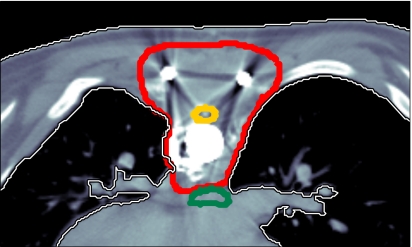
We illustrate results for a paraspinal tumor, which is shown in Fig. 1. The tumor entirely surrounds the spinal cord which is to be spared. Additional organs at risk are the esophagus, the lungs and the remaining unclassified tissue. The patient has metal implants due to surgery prior to radiotherapy, which cause artefacts in the planning CT image and contribute to the range uncertainty.
Figure 1.
Paraspinal case: The thick contours correspond to the CTV, the spinal cord, and the esophagus.
IMPT technique
We choose three beam direction: a posterior beam at 0° and two oblique beams at ±45°. IMPT treatment plans for the 3D spot scanning technique according to the classification by Lomax17 are optimized. We precalculate dose distributions of pencil beams placed on a regular grid of 5 mm resolution in both lateral directions and at preselected energy layers which correspond to 5.0 mm difference in water equivalent range. We use a previously published pencil beam algorithm18 which uses a subpencil-beam decomposition approach to account for lateral density heterogeneities. As the level of lateral heterogeneities is very high for this case, a high number of subpencil-beams (121 per pencil beam) is to be applied.19 We assume a 5 mm sigma of the parallel Gaussian pencil beam at patient surface.
Objective function
We apply a quadratic objective function to optimize a treatment plan
| (6) |
where is the prescribed dose to the CTV and is the desired dose to all critical structures. ∣Vn∣ is the number of voxels in Vn, which is the set of voxels belonging to the volume of interest with index n. The penalty factors αn that weight the objectives for different organs are chosen in such a way that for the conventional IMPT plan the maximum dose to the spinal cord and the esophagus is about 50 Gy. All other structures play only a minor role and their penalty factors are chosen small enough so that CTV coverage was not substantially compromised by their objectives. All treatment plans in this article are optimized with the same set of penalty factors. The penalty factors are summarized in Table 1.
Table 1.
Summary of weighting factors, sampling rates, and number of voxels for all volumes of interest.
| Penalty αn | Sampling rate pn | No. voxels ∣Vn∣ | |
|---|---|---|---|
| CTV | 200 | 0.1 | 14 466 |
| Spinal cord | 6 | 1.0 | 815 |
| Esophagus | 1 | 1.0 | 1538 |
| Left lung | 10 | 0.05 | 57 217 |
| Right lung | 10 | 0.05 | 72 557 |
| Heart | 10 | 0.05 | 35 916 |
| Unclassified tissue | 10 | 0.05 | 713 827 |
Quantification of the uncertainty
For this study, we assume a range uncertainty of σj=5 mm for all pencil beams and a systematic setup error of 2.5 mm which is uncorrelated in all three spatial dimensions [i.e., the diagonal elements of Cs in Eq. 3 are (2.5 mm)2 and all nondiagonal elements are zero].
We make generic assumptions on the amount of range uncertainty due to the lack of measured data to support more sophisticated models. Regarding the various potential sources of range uncertainty including uncertainty in stopping power, metal implants, CT artifacts due to implants, or weight loss∕gain, 5 mm uncertainty is expected to be worth accounting for. Future research may aim at deriving more precise uncertainty models for specific tumor sites and planning protocols, based on future studies that put tighter bounds on the actual magnitude of the range error. Further discussion on aspects of the range uncertainty model is provided in Appendix A.
A numerical value for a range error refers to an error in water equivalent range. In order to simulate the dosimetric effect of a 5 mm range overshoot, we substitute the dose distribution of a pencil beam by a pencil beam with higher primary proton energy (where the difference in primary proton energy corresponds to 5 mm water equivalent range). This effectively models a change of 5 mm in radiological path length in the plateau region of the pencil beam, which could occur for various reasons (that are not explicitely modeled here). Typically, there may be one CT scan of the patient that is used for treatment planning. The nominal range in Eq. 1 is then given by beamlet range calculated based on that one planning CT scan.
Approximation of dose distributions for range and setup errors
In order to evaluate the objective function (4), we have to calculate the dose distribution for a given setup error and a given range deviation. Practically, it may often be unrealistic to perform an online dose calculation from scratch, especially if sophisticated and accurate dose calculation methods are to be applied. Therefore, the dose distribution for a range or setup error has to be approximated. In Appendix C we describe multiple options to do this. For the results discussed in Secs. 4, 5, we use an approach that approximates the dose distribution of a beamlet in a shifted patient by using neighboring beamlets and virtual beamlets as described in detail in Appendices C1c, C2b.
Solving the optimization problem
To solve the optimization problem, we apply a stochastic gradient descent algorithm. In order to calculate the gradient of the objective function exactly, one has to perform a summation over all voxels and all scenarios (setup errors and range shift combinations), which is too time consuming. In order to make the optimization problem tractable, we estimate the gradient of the objective function by using voxel sampling and scenario sampling. Only a subset of the voxels and a subset of the scenarios are used to provide an estimate of the gradient. A projection method is applied to handle the non-negativity constraint for the beamlet weights.
To obtain the results shown in this article, we applied the voxel sampling rates pn shown in Table 1. In each optimization step, we generated ten scenarios based on the probability distributions in Eqs. 2, 3. For each scenario a different set of voxels is drawn randomly. The objective function value and its gradient with respect to the beamlet weights are estimated by averaging over the ten scenarios. Specifically, the estimate of the objective is given by
Here, ψik∊{0,1} is a binary random variable with probability distribution P(ψik=1)=pn and P(ψik=0)=1−pn, where n is the index to the volume of interest that voxel i belongs to. Δsk and δk are random variables for setup and range errors, that obey the probability distributions in Eqs. 3, 2, respectively. A previous publication20 discusses the performance of the algorithm in the context of voxel sampling alone and presents an algorithm to automatically tune the voxel sampling rates. A generalization of this method to the combination of voxel and scenario sampling is subject of ongoing research.
Stochastic gradient descent has been implemented into our in-house IMRT∕IMPT optimization software previously reported on.21 The software is implemented in C++ according to principles of object oriented programming. Stochastic gradient descent can be used to optimize IMRT∕IMPT in the context of optimizing the expected value of an objective function which depends on uncertain parameters. Due to the modular structure of the software, the concept can be applied to various types of uncertainty. Those include systematic setup and range errors as demonstrated in this article. Other applications that have been implemented are random setup errors and variations in the breathing pattern for 4D optimization for lung and liver tumors.
Size of the problem
For the paraspinal case presented here, the total number of beamlets is 12 775. The total number of voxels is 896 336 (see Table 1) and the total number of nonzero elements in the dose contribution matrix (see Appendix C) is 38 659 890. For the plan that incorporates both range and setup errors, the total number of virtual beamlets is 221 337 (see Appendices C1c, C2b). Improving the resolution of the beamlet grid from 5 to 2.5 mm requires eight times as many beamlets. In addition, beamlets have to be added at the periphery. The total number of nonzero elements in the dose contribution matrix is 826 775 673—thus requiring approximately 6.6 Gbytes of memory, if each entry is stored as a 4-byte-float for the dose value and a 4-byte-int for the voxel index.
RESULTS OF PROBABILISTIC TREATMENT PLANNING
In this section, we analyze treatment plans obtained by applying the probabilistic approach to the paraspinal case in Fig. 1. We compare four 3D spot scanning IMPT treatment plans:
a “conventional” IMPT plan that does not account for any uncertainty,
a plan that accounts for range uncertainty only,
a plan that accounts for setup errors only, and
a plan that accounts for both range uncertainty and setup errors.
Sensitivity of conventional treatment plans
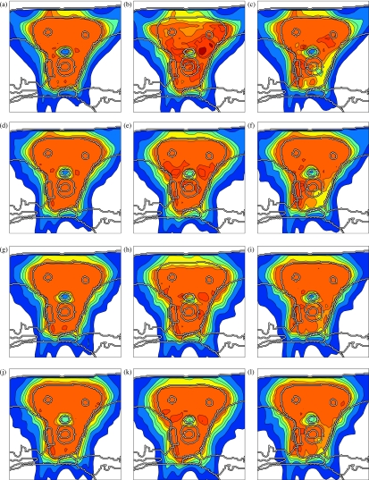
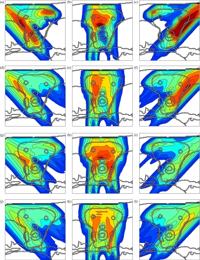
Figures 5a, 4a, 4b, 4c shows a conventional IMPT treatment plan, which is optimized without taking uncertainty into account. Figure 5a shows the cumulative dose of all three beams for the nominal range and the nominal setup position, and Figs. 4a, 4b, 4c show the corresponding dose contributions of the beams at 0° and ±45°. If no error occurs, a very homogeneous dose distribution can be delivered to the CTV and a good sparing of the spinal cord can be achieved. If we perform a sensitivity analysis of the plan, we observe that the dose distribution in Fig. 5a is highly degraded. Figure 5b shows the resulting dose distribution for an overshoot of 5 mm in water equivalent range (i.e., the Bragg peak positions of all beamlets are shifted further into the patient). This sensitivity can be explained by analyzing the dose contributions of individual beam directions. Figures 4b, 4c show the dose contributions of the beams at 0° and 45° for no setup or range error. The optimization assigns a high weight to Bragg peaks placed in front of the spinal cord. This allows for the best dose sparing of the critical structure as the steep distal falloff of the Bragg peak is utilized. As a consequence, a very high dose is delivered to the spinal cord if the range of a pencil beam is larger than expected. Generally, dose gradients in beam direction make the plan very sensitive to range variations.
Figure 5.
Sensitivity analysis of the four treatment plans: (a)–(c) conventional IMPT plan, (d)–(f) IMPT plan optimized for range uncertainties alone, (g)–(i) IMPT plan optimized for setup errors alone, (j)–(l) IMPT plan optimized while accounting for both setup and range uncertainty; the three columns show the nominal dose distribution [(a), (d), (g), (j)], the dose distribution resulting from a systematic overshoot of 5 mm in water equivalent range [(b), (e), (h), (k)], and a systematic setup error of 2.5 mm rightwards [(c), (f), (i), (l)]. The color scale in Fig. 2c applies.
Figure 4.
Dose contributions of the individual beams for four treatment plans: (a)–(c) conventional IMPT plan, (d)–(f) IMPT plan optimized for range uncertainties alone, (g)–(i) IMPT plan optimized for setup errors alone and (j)–(l) IMPT plan optimized while accounting for both setup and range uncertainty. The color scale in Fig. 2c applies.
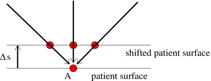
Figures 25c illustrate that the treatment plan is also sensitive to setup errors. Figure 2a shows the resulting dose distribution for a 3.5 mm setup error posteriorly. The rigid shift of the patient has no impact on the dose delivered by the beam at 0°. However, the oblique beams at ±45° hit the patient surface at a different position. This is illustrated schematically in Fig. 3. Their dose contributions are shifted relative to each other and consequently do not add up to a homogeneous dose distribution in the CTV. In this case, the oblique beams at ±45° are shifted apart and cause cold spots around the spinal cord. For a patient shift of 3.5 mm anteriorly, the dose contributions of the oblique beams at ±45° are shifted towards each other and, among other effects, overdose the spinal cord and cause a hot spot anterior to the spinal cord [Fig. 2b]. Figure 5c shows the resulting dose distribution for a setup shift of 2.5 mm rightwards. For a radiologically homogeneous patient, a shift of the patient would mainly cause a shift of the cumulative dose distribution. Since the shift is approximately parallel to the patient surface, it affects all beams in the same way and does not lead to a misalignment of their dose contributions. However, the resulting dose distribution is also strongly influenced by the misalignment of density inhomogeneities. This particularly applies to the metal implants present in this case. As a consequence, underdosage of the tumor does not only occur at the boundary of the CTV, but also in regions deeper within the CTV.
Figure 2.
Sensitivity analysis of a conventional treatment plan: (a) dose distribution that results from a 3.5 mm setup error posteriorly, (b) dose distribution realized for a 3.5 mm setup error anteriorly, (c) color scale for cumulative dose distributions (left) and dose contributions of individual beams (right) in percent of the prescribed dose.
Figure 3.
Illustration of the effect of misaligned beams. In this schematic example, three pencil beams hit the patient surface at point A. For a setup shift Δs, the three beams hit the patient surface at different points, and hence, yield a different dose distribution.
Although this section analyzes a treatment plan that does not apply a margin to the CTV, it is evident that the PTV concept cannot solve the problem sufficiently. A PTV margin around the CTV could only reduce the underdosage of the CTV at the boundary due to geometric shifts of the dose distribution. It cannot account for dose inhomogeneity in the CTV and overdosage of the spinal cord due to misalignments of beams and density heterogeneities. Defining a PTV has no influence on the occurrence of steep dose gradients (within the dose distribution of a single beam) inside the CTV, as would be necessary to improve the robustness of a treatment plan. In addition, the dose distribution around the spinal cord cannot be controlled by a PTV approach since a margin extension of the CTV at the transition to the spinal cord would simply eliminate the structure to be spared.
Accounting for range uncertainty
Figures 5d, 4d, 4e, 4f shows the treatment plan that was optimized for a Gaussian range uncertainty of 5 mm standard deviation. The treatment plan is qualitatively different from the conventional plan. As apparent in Figs. 4d, 4e, 4f, the dose contributions of individual beams are more homogeneous in beam direction, steep dose gradients are avoided. Consequently, a shift of these dose distributions in beam direction has little impact on the dose distribution in the CTV. Instead of the distal falloff, the lateral falloff of the pencil beam is used to avoid the spinal cord. Therefore, the spinal cord is protected from being overdosed in the case of a range overshoot. Figure 5e shows the dose distribution that is realized for a 5 mm range overshoot. As apparent, the sparing of the spinal cord is preserved and the dose in the CTV remains widely homogeneous. The robustness against range errors can be achieved without noticably compromising dose homogeneity in the CTV for the nominal case [Fig. 5d]. A plan optimized for range uncertainty may still be sensitive to setup errors as apparent in Fig. 5f, which shows the dose distribution for a 2.5 mm setup error rightwards.
Accounting for setup errors
A treatment plan optimized for systematic setup errors only is substantially different from a conventional treatment plan or a plan optimized for range uncertainty [Figs. 4g, 4h, 4i]. In this case, the dose distribution in the CTV is sensitive to dose gradients in the direction parallel to the patient surface. In order to make the plan robust against setup errors, dose gradients in the left-right direction have to be avoided. This is reflected in Figs. 4g, 4h, 4i. Figure 5i demonstrates the robustness of the treatment plan for 2.5 mm setup error rightwards. Dose coverage and homogeneity in the CTV is well preserved. As expected, a plan optimized for setup errors alone may still be sensitive to range errors. Figure 5h shows the overdosage of the spinal cord for a 5 mm range overshoot. The reason for this can be understood from Fig. 4h which shows the dose contribution of the beam at 0°. The distal edge of Bragg peaks is placed directly in front of the spinal cord. This does not cause problems regarding setup errors because for no rigid shift of the patient this dose can be shifted into the spinal cord.
Incorporating both range and setup uncertainty
A treatment plan that is robust against both setup and range errors has to combine the requirements of both types of uncertainty. This is possible to some degree. As apparent in Figs. 4j, 4k, 4l, the dose contributions of individual beams are relatively smooth in both the left-right direction and the beam direction in order to ensure a widely homogeneous dose in the CTV. Regarding range uncertainty, using the lateral falloff of the Bragg peak is better than using the distal falloff. However, regarding setup uncertainty, the distal falloff may be more favorable. In this respect not all requirements can be met by a single treatment plan. Figures 5k, 5l show widely homogeneous dose distributions in the CTV and reasonable sparing of the spinal cord for a 5 mm range overshoot and a 2.5 mm setup error rightwards, respectively. For the nominal case, one can still obtain a homogeneous dose in the CTV [Fig. 5j].
Summary
Conventional IMPT plans are sensitive to setup and range errors due to steep dose gradients in the dose distribution of a single field. Incorporating uncertainty into IMPT optimization yields substantially more robust treatment plans by redistributing dose among different fields and by avoiding unfavorable in-field dose gradients. Plans optimized for range uncertainty specifically avoid dose gradients in beam direction, plans optimized for setup errors avoid dose gradients in the left-right direction (for the patient geometry investigated here). A plan optimized for both types of uncertainty tries to avoid (or smoothen) gradients in all directions. The discussion in this section is focused on the spinal cord and the CTV. A similar analysis can be performed for the esophagus. It supports the above findings.
Remarks
In this article, we present a detailed case study for generic assumptions on the range uncertainty, i.e., 5 mm for each beamlet. Future research may aim at deriving more precise uncertainty models for specific tumor sites and planning protocols, in order to optimize the tradeoff between robustness and nominal plan quality (see Sec. 5).
Particularly, the range uncertainty model requires several assumptions which are not well supported by available measured data (see also Appendix A). Generally, the optimal plan depends on the uncertainty model and parameters therein. However, the lack of precise knowledge of the range uncertainty does not question the usefulness of the proposed methods per se. More robust plans are obtained mainly by reducing unfavorable dose gradients. This is achieved by many uncertainty models for a wide range of parameter values. Compared to conventional plans that do not account for uncertainty at all, the robustness of plans can be expected to improve even if the uncertainty model is an idealization of the unknown reality.
Computation time
Optimization of the conventional plan took 10 min (on a Dell Precision 690 workstation with 16 GB RAM). Optimization of the plan that incorporates range and setup errors plan took 4 h. The plans that account for only range uncertainty and only setup errors required intermediate computation times of 1 h and 2 h, respectively. See Sec. 3G regarding the size of the optimization problem.
For all treatment plans, the optimization was run for 20 h. The computation times stated above refer to the intermediate results that show almost no difference in the dose distributions of individual beams compared to the result after 20 h.
Those numbers are meant to be rough guidelines and we did not aim at optimal computational performance. We expect to achieve substantial further speed up by various approaches. Those include a modified implementation, tuned sampling rates for voxels, and scenarios as mentioned in Sec. 3F, using fewer scenarios, and also by stopping the optimization after fewer iterations. Acceptable treatment plans that show the characteristic features of the final results were obtained for much shorter computation times. The values for computation time refer to the optimization alone and do not include the calculation of the dose contribution matrix.
TRADING OFF ROBUSTNESS AND NOMINAL PLAN QUALITY
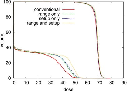
As pointed out in Sec. 2C, the probabilistic approach inherently leads to a multicriteria optimization problem. In order to achieve robustness, one will in general have to compromise plan quality for the nominal case to some extent. This can be seen in Fig. 6 which shows the DVHs of the nominal dose distributions for the four treatment plans in Figs. 4a, 4d, 4g, 4j. The conventional plan yields the best sparing of the spinal cord and the best CTV coverage for the nominal scenario, because it is optimized specifically for this one scenario.
Figure 6.
DVH comparison of the four treatment plans for the nominal case, that is no range or setup error occurs. DVHs for the CTV and the spinal cord are shown.
The plan optimized for range uncertainties takes scenarios for under- and overshoot into account via additional terms in the objective function. It thereby improves plan quality for the case that a range deviation occurs and compromises plan quality for the nominal case. In the case of range uncertainty, the physical reason of the price associated with robustness is evident: in order to ensure sparing of the spinal cord for the case of range overshoot, one has to utilize the lateral falloff of the Bragg peak to shape the dose distribution at the boundary of spinal cord and OAR. For typical beam sizes (5 mm sigma at patient surface was used in this study), the lateral falloff of the Bragg peak is more shallow compared to the distal falloff. Hence, for the nominal case, CTV coverage or dose burden of the spinal cord are compromised.
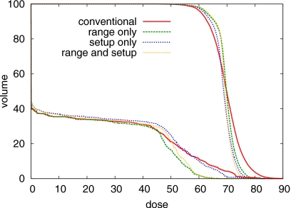
On the other hand, probabilistic treatment plans are substantially more robust against errors. Figure 7 shows the DVHs of the dose distributions for a 5 mm range overshoot. For the conventional plan, the maximum dose in the spinal cord exceeds the prescribed dose to the tumor. In contrast, the probabilistic plan that accounts for range uncertainty preserves a good sparing of the spinal cord.
Figure 7.
DVH comparison of the four treatment plans for an overshoot of 5 mm in water equivalent range. DVHs for the CTV and the spinal cord are shown.
Accounting for a setup error in all directions also compromises the dose distribution for the nominal case (Fig. 6). This can be understood by considering a setup error in left-right direction. For the patient geometry and the beam arrangement as chosen here, it is not possible to deliver the dose in such a way that the dose distribution is insensitive to patient shifts in the left-right direction. No matter how the dose is distributed among the beams, a setup error in the left-right direction will shift the spinal cord into the adjacent high dose region. By carefully regarding the isodose lines around the spinal cord in Fig. 5g, it can be observed that the probabilistic treatment plan handles this situation by reducing the dose gradient between spinal cord and the CTV. This prevents very high maximum doses in the spinal cord for the case that a setup error occurs, but compromises the plan for nominal case.
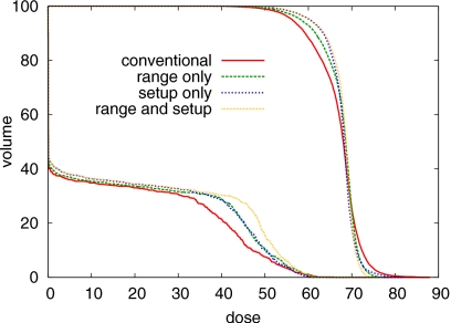
On the other hand, the plan optimized for setup errors yields a much better CTV coverage for the case that a setup error occurs. This is apparent in Fig. 5i and in the DVH comparison in Fig. 8. Whereas the conventional plan and the plan that only accounts for range uncertainty show severe underdosage of the CTV, this is substantially reduced for the plans that incorporate setup errors in the optimization.
Figure 8.
DVH comparison of the four treatment plans for a setup error of 2.5 mm rightwards. DVHs for the CTV and the spinal cord are shown.
In summary, treatment planning for IMPT does not only involve a trade-off between objectives for different organs. It also involves a trade-off between robustness and plan quality for the nominal case. Improving robustness is clearly desirable as long as it does not substantially compromise plan quality for the nominal case. Compromising nominal plan quality to achieve robustness against very large errors that are extremely unlikely to occur is undesirable. Quantifying the uncertainty for a given clinical protocol helps to set limits on the amount of robustness needed, but it does not per se determine a specific trade-off between nominal plan quality and robustness. This may remain the responsibility of the treatment planner.
As a consequence, the aspect of robustness should be reflected in dose reporting protocols. Reporting only the dose for the nominal case neglects essential aspects of a treatment plan. The nominal scenario is only one possible realization and may not describe the quality of a treatment plan well.
A large variety of surrogates can be considered for visualization of plan quality and robustness in the presence of uncertainty, for the purpose of both plan evaluation and reporting. Those include dose distributions for specific realizations of range and setup errors, the standard deviation distributions as a measure of the uncertainty of the dose in each voxel,5 worst case dose distributions and maximum error distribution,7 probability distributions for EUD, TCP, and NTCP values, or the probability that the dose in a voxel is within a dose interval of interest.16
CONCLUSIONS
In this article, we show that conventional IMPT plans, which are optimized without accounting for range and setup accuracy, may be very sensitive to errors. Degradation of the dose distribution is mainly due to a shift of the dose contributions of individual beams relative to each other and by misaligned density heterogeneities which alter the dose deposition of a single field for a setup error. Therefore, the problem cannot be solved sufficiently by a margin approach (Sec. 4A).
The probabilistic approach is applied to incorporate setup errors and range uncertainty into the optimization of an IMPT treatment plan. It is shown that robustness of a plan against errors is achieved by redistributing the dose contributions among different beam directions. In order to achieve robustness against range errors, dose gradients in beam direction in the dose distribution of a single field have to be avoided. Specifically, placing the distal falloff of a Bragg peak directly in front of an OAR is avoided. In order to achieve robustness against setup errors, lateral gradients within a field have to be avoided. Treatment plans that are optimized for range errors only may be qualitatively different from treatment plans optimized for setup errors only as both types of uncertainty require different features of a treatment plan to achieve robustness. A plan that is optimized for both range and setup errors combines the requirements for robustness against setup and range errors as far as possible.
Methods to directly incorporate uncertainty into inverse planning are of particular importance in IMPT as the safety margin concept (as typically applied in photon therapy) is neither suitable for handling range uncertainty nor setup errors.
ACKNOWLEDGMENTS
This research was supported in part by Siemens Medical Solutions, Germany, by the US National Cancer Institute under Grant Nos. P01-CA21239 and R01-CA103904, the United States-Israel Binational Science Foundation (BSF) under Grant No. 2003275, the US National Science Foundation under Grant No. ECS-0312921, the US National Institutes of Health under Grant No. R01-CA118200, the Deutsche Forschungsgemeinschaft under Grant No. 33∕8-2 and CMS Inc., St. Louis, USA. Parts of this work were presented at the ICCR conference in 2007 (Ref. 26) and the annual AAPM meeting 2007.27
APPENDIX A: MOTIVATION OF THE UNCERTAINTY MODEL
The characterization of the setup uncertainty is relatively concise. It only requires six independent parameters in the covariance matrix Cs in Eq. 3. The model of range uncertainty in turn is more complex. In the formulation of Sec. 2A, we may specify the amount of uncertainty σj for each beamlet, and in addition, correlations between the range shift of beamlets. For the time being, there will not be sufficient experimental data to specify these parameters. Therefore, the model of uncertainty is partly based on heuristic assumption, some of which are discussed in more detail below.
Considering systematic errors
Considering range uncertainty as a systematic error (in the sense that the same range error is realized in every fraction) is a simplification. Whereas range errors due to imperfections of the planning CT are systematic, errors due to weight loss or weight gain are not constant over time. Hence, in different fractions, the range error realization may be different. Treating range uncertainty purely as a systematic error is a conservative approach as this method aims at a high quality dose distribution for every realization of the error—independent of the error realization in other fractions. Incorporating a more detailed model for variations of the range uncertainty during the course of treatment could theoretically improve the plan—but only if this model was correct, which is difficult to ensure.
The role of the shape of the probability distribution
We choose a Gaussian distribution for range and setup error. This is mostly due to lack of better knowledge. (To some extent, this can be formalized in information theory by Jaynes principle of the unbiased guess:22 the Gaussian distribution minimizes the Shannon information under the assumption that the random variable is characterized by mean and standard deviation.) However, in the context of systematic errors, the exact shape of the probability distribution is not very critical. This can be understood by interpreting the objective function in a multicriteria context (Sec. 2C): the probability distribution only determines the trade-off between plan quality for different scenarios. Not knowing the probability distribution accurately only means that we might not choose the best trade-off between plan quality for different scenarios. But if we have a plan that is reasonably good for all realistic scenarios, then the realization of a favorable cumulative dose distribution at the end of the treatment does not depend on the correctness of the shape of the probability distribution. (Note that this is different for incorporating random errors23 or respiratory motion in IMRT, where the expected cumulative dose distribution is approximately given by a convolution of the nominal dose with the probability distribution.)
Beamlet dependent range uncertainties
In this work, we assumed the same range uncertainty σj for each beamlet. The concept and our implementation allow for beamlet dependent range uncertainty. However, this would require more detailed assumptions on the cause of range uncertainty and will be tumor site specific. A potential improvement for paraspinal cases could be attained by assuming larger range uncertainty for beamlets that pass directly through metal implants.
For beamlet dependent range uncertainties, the range uncertainty σj for a beamlet j would be a function of the setup error Δs. In this case, it could be assumed that a fixed range uncertainty σ is associated with every virtual beamlet (see Appendix C1c) as a virtual beamlet passes through a defined region of tissue. The dependence of the range uncertainty of the real beamlet on the setup error would therefore not represent a problem for solving the optimization problem. The setup error and the range shift of a virtual beamlet could be considered statistically independent.
The correlation of beamlet range shifts
We have to make assumptions about the correlation of range variations of different beamlets. In many cases (although not always), it may be reasonable to assume that beamlets at the same lateral position (i.e., they differ only in the primary proton energy) are correlated. This is because they are affected by the same tissue for most parts. Beamlets at different lateral positions can in general have different range errors. If CT artifacts due to metal implants were the primary source of range uncertainty, different beamlets would be affected by different artifacts and would have different range errors. If, on the other hand, weight loss or errors in the conversion of Hounsfield units to stopping power were the primary source of range uncertainty, there would be a stronger correlation between the range errors of beamlets. In this case, beamlets would tend to all overshoot or all undershoot. Hence, further specification of the correlation model would require more explicit assumptions on the origin of range uncertainty. This was avoided here. For this patient, we analyzed the impact of the correlation model, which is reported on in Appendix B.
APPENDIX B: THE IMPACT OF THE BEAMLET CORRELATION MODEL ON THE TREATMENT PLAN
For this patient, we investigate the impact of the beamlet correlation model for the range errors on the treatment plan. Different beamlet correlation models correspond to specifications of the nondiagonal elements of (Cρ)jk in Eq. 2. We consider three models:
Model 1: all beamlets are correlated: (Cρ)jk=1 for all beamlets j and k.
Model 2: beamlets within one beam direction are correlated as described in Sec. 2A. This is the correlation model used throughout the article.
Model 3: beamlets are correlated [(Cρ)jk=1] if they correspond to the same lateral position in the same beam direction, and uncorrelated otherwise [(Cρ)jk=0]. Correlated beamlets differ only in their primary proton energy.
We optimize treatment plans assuming a range uncertainty of σj=5 mm for all beamlets and no setup error. The plans turn out to be qualitatively similar, i.e., dose gradients in beam direction are reduced compared to the conventional plan. (The dose contributions of individual beams are not shown here as they provide little insight.) An intuitive explanation is that the robustness of the treatment plan benefits from the reduction of steep dose gradients in beam direction, independent of the details of the correlation model.
In order to compare the robustness of the treatment plans with respect to the three range uncertainty models defined above, we calculate the standard deviation of the dose in each voxel as a measure of the dose uncertainty. The standard deviation in voxel i is given by the square root of the variance , where ⟨Di⟩ is the expectation of the dose in voxel i taken over all range error realizations. Practically, the standard deviation was calculated via Monte Carlo integration by generating 1000 random scenarios.
Figure 9 shows the standard deviation calculated using correlation model 2 for three treatment plans: (a) the plan optimized using correlation model 2 shown in Figs. 4d, 4e, 4f (b) the plan optimized for correlation model 3, and (c) the conventional plan shown in Figs. 4a, 4b, 4c. The dose uncertainty (with respect to correlation model 2) is smallest for the plan that was optimized incorporating that model. The dose uncertainty for the plan optimized for correlation model 3 [Fig. 9b] is larger because the corresponding plan was optimized for correlation model 3, but is now evaluated with respect to model 2. The plan does not protect as well against errors where all beamlets of a beam direction over-or undershoot simultaneously because these scenarios are less likely for correlation model 3. Nonetheless, it is still more robust than the conventional plan which shows a much larger dose uncertainty all over the CTV and especially around the spinal cord [Fig. 9c].
Figure 9.
Standard deviation of the dose for three treatment plans discussed in Appendix B: (a) optimized for beamlet correlation model 2, (b) optimized for model 3, (c) conventional plan. The color scale is in percent of prescribed dose.
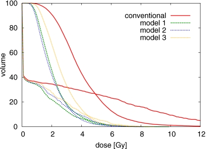
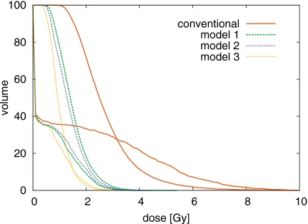
The standard-deviation-volume histogram (SDVH), i.e., the fraction of the volume featuring a dose uncertainty of more than a certain number of Gy, provides a more quantitative comparison of the plans in terms of dose uncertainty. We consider the conventional plan and three plans optimized for range uncertainty using the models 1–3. Figure 10 shows the SDVH recalculated according to correlation model 2, confirming the discussion about Fig. 9. Figure 11 shows the SDVH of the same plans recalculated according to correlation model 3. The dose uncertainty is similar for the three plans that incorporate some range uncertainty model into the optimization, but is substantially larger for the conventional plan.
Figure 10.
SDVH comparison for CTV and spinal cord for the treatment plans discussed in Appendix B. The standard deviation of the dose is calculated using correlation model 2.
Figure 11.
SDVH comparison for CTV and spinal cord for the treatment plans discussed in Appendix B. The standard deviation of the dose is calculated using correlation model 3.
These three correlation models can be considered as idealized extreme cases. Equation 2 is more general and does also allow for mixtures of these extreme cases [0<(Cρ)jk<1], which is more realistic. However, all treatment plans that account for some range uncertainty model are more robust than the conventional plan, independent of correlation model the plan is evaluated for.
APPENDIX C: APPROXIMATING DOSE DISTRIBUTIONS
In order to evaluate the objective function, we have to calculate the dose distribution for a given setup error and a given range deviation. Practically, it may often be unrealistic to perform an online dose calculation from scratch, especially if sophisticated and accurate dose calculation methods are to be applied or the number of scenarios is large. Therefore, the dose distribution for a setup or range error has to be approximated. We assume that we precalculate the dose distributions of individual pencil beams assuming that the nominal range is realized and the patient is in its nominal position. The dose at a point r=(xy,z) in the patient is then given by
| (C1) |
where d(r,b) denotes the dose contribution of a beamlet characterized by b to the point r in the patient. The vector b=(x,y,e) contains the x and y coordinate of the beamlet position in a beams-eye-view coordinate system and e denotes the primary proton energy. The matrix with elements dij=d(ri,bj), where ri is the position of the voxel i, is referred to as the dose contribution matrix.
Setup errors
In order to incorporate setup errors into the optimization, we need to efficiently calculate d(r,b∣Δs), the dose distribution of a beamlet for a setup error Δs. This can be performed using different approximations.
The static dose cloud approximation
In the static dose cloud approximation, as often applied in photon therapy, we approximate the dose contribution to a patient who is shifted by Δs according to
| (C2) |
Usually, we do not have a precalculated dose value for the point r+Δs. Therefore, we approximate the dose value using the precalculated dose to the nearest voxel. Alternatively, trilinear interpolation can be used. This approximation does neither account for the fact that the dose distribution is shifted with the patient for a setup error in beam direction, nor for potential misalignments of tissue heterogeneities. For IMPT optimization, this approximation turns out to be insufficient (results not shown in this article).
An improved static dose cloud approximation
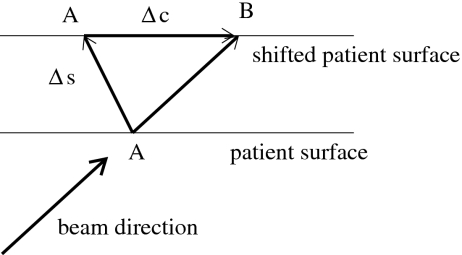
The static dose cloud approximation can be improved if we account for the effect that the dose cloud may be shifted within the patient. If the patient moves, the pencil beam will hit the patient surface at a different position as illustrated in Fig. 12. For the patient in nominal position, the pencil beam hits the patient surface at point A. If the patient is shifted by Δs, the pencil beam hits the patient at point B, which is shifted relative to A by the vector Δc which we have to compute. It turns out that
| (C3) |
where eb is a unit vector in beam direction and en is a unit normal vector on the patient surface which is assumed to be flat in the vicinity of point A. We can now approximate the dose distribution d(r,b∣Δs) by
| (C4) |
This approach reproduces some required features. For the special case that the setup shift Δs is parallel to the beam direction, the dose distribution in the patient would not change. If the setup shift is parallel to the patient surface, the correction vector Δc is equal to −Δs. However, this approximation would only be accurate for a patient without tissue inhomogeneities. It does, for example, not account for the problem that a dense structure like a titanium rod may move into the path of the beamlet.
Figure 12.
Illustration of the improved static dose cloud approximation: For a setup error Δs, the entrance point of the pencil beam is shifted by Δc on the patient surface.
Approximating dose contributions based on virtual beamlets
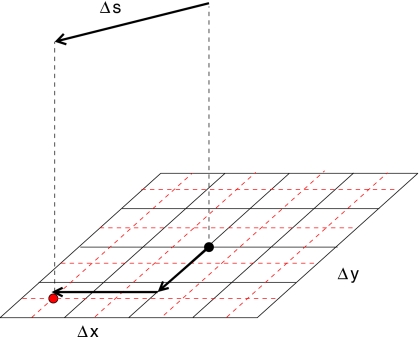
In Secs. C.1.a and C.1.b we approximate dose distributions by applying an effective shift to a voxel. Alternatively, we can apply a shift to the beamlet grid as illustrated in Fig. 13. We look at the setup shift Δs in the beams-eye-view coordinate system and project it onto a plane perpendicular to the beam direction. For a parallel beam, we have
| (C5) |
with Δb=(Δx,Δy,0). This is not an approximation but holds exactly. However, we usually will not have a precalculated dose distribution for a pencil beam at position b+Δb. Therefore, we approximate d(r,b+Δb) by taking the precalculated pencil beam that is closest to b+Δb.
Figure 13.
Illustration of dose approximation using virtual beamlets: The dose distribution of the “real” beamlet marked by the central dot is approximated by the virtual beamlet marked by the dot at the lower left.
In this article, lateral distance of two beamlets is 5 mm in both x and y direction. In order to model setup errors reasonably accurate, we have to precalculate the dose distributions of additional, virtual beamlets, which are not delivered and not associated with a weight to be optimized. They are only used to approximate dose distributions in a shifted patient. In this work, we additionally place virtual beamlets on a finer grid with 2.5 mm resolution.
Discussion
The virtual beamlet approach has the potential to approximate the dose distribution in a shifted patient most accurately. There are, however, some disadvantages and limitations. First, the approach requires that virtual beamlets are placed at a sufficiently small distance and that the corresponding dose distributions are assessible during the optimization. This increases the memory requirements of the computer and limits the clinical cases that are computationally tractable on regular hardware. Second, it can only be applied to rigid shifts of the patient. It cannot be generalized to model internal deformations. For the method in Appendices C1a, C1b, this would to some extent be possible. It is therefore worthwhile to investigate the potential of the improved static dose cloud approximation described in Appendix C1b.
Applicability to IMRT with photons
The methods in Appendices C1a, C1b, C1c are also applicable to IMRT optimization in photon therapy. See also Beckham et al.24 for dose convolution versus fluence convolution to account for random errors. Although, the principal limitations of the static dose cloud method (Appendix C1a) are apparent, deviations from the static dose cloud approximation are relatively small in photon IMRT (see, e.g., Ref. 25). Therefore, the expected benefit of using the more advanced methods of Appendices C1b, C1c is moderate in IMRT, whereas it is essential in IMPT. This is partly due to the larger number of (roughly equally spaced) beams used in IMRT and less severe dose gradients in the dose contributions of these beams.
Range errors
For range errors, we can also approximate dose distributions by either applying shifts to voxels or shifts to beamlets.
Voxel shift based approximation method
In order to approximate the dose distribution d(r,b∣δ) of a beamlet for a range overshoot δ, we can assume
| (C6) |
where we can approximate d(r−δeb,b) by trilinear interpolation of the voxel doses next to the point r−δeb or by the dose in the nearest voxel. In this formulation, the range error δ represents a geometrical shift of the pencil beam dose distribution in beam direction. This has some limitations in the presence of density heterogeneities. For example, we do not model the effect that a pencil beam that overshoots into lung tissue propagates further into the patient than it would in soft tissue.
Virtual bixel method
Alternatively, we can interpret the range error as an error in water equivalent range. The range shift δ corresponds to a change Δe in primary proton energy. We then have
| (C7) |
where Δb=(0,0,Δe). In this work, we place real beamlets at energy layers of 5 mm water equivalent range difference. In addition, we place virtual beamlets on energy layers at 2.5 mm water equivalent range difference.
APPENDIX D: THE IMPACT OF THE DOSE APPROXIMATION TECHNIQUE ON THE TREATMENT PLAN
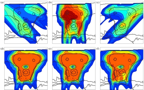
Figure 14 shows a treatment plan that is optimized for a Gaussian setup error of 2.5 mm in all dimensions by using the improved static dose cloud approximation to approximate the dose distribution in a shifted patient. For comparison, the plan optimized using the virtual bixel approximation is shown in Figs. 4g, 4h, 4i, 5g, 5h, 5i. By comparing the dose contributions of the individual beam directions, it can be noted that both plans are similar. The treatment plan using the improved static dose cloud approximation reproduces important features to achieve robustness against setup errors, i.e., the avoidance of steep dose gradient in the left-right direction. Figure 14e shows the dose distribution for a 2.5 mm setup error rightwards as predicted by the improved static dose cloud approximation. According to this approximation, good CTV coverage is preserved. However, substantial underdosage of the anterior part of the CTV is observed if the dose distribution for a 2.5 mm setup error is recalculated with the virtual bixel model which accounts for misaligned density heterogeneities. In conclusion, the improved static dose cloud approximation yields adequate results for cases without major density heterogeneities (not shown here), but has limitations in the presence of metal implants.
Figure 14.
Treatment plan optimized for a Gaussian setup error of 2.5 mm while approximating dose distributions for setup errors by the improved static dose cloud approximation (Appendix C1b): (a)–(c) dose contributions of individual beams, (d) dose distribution for the nominal case, (e) dose distribution for a 2.5 mm setup error rightwards predicted by the improved static dose cloud approximation, and (f) dose distribution for a 2.5 mm setup error rightwards predicted by the virtual bixel approximation method. The color scale in Fig. 2c applies.
References
- Schneider U., Pedroni E., and Lomax A., “The calibration of CT Hounsfield units for radiotherapy treatment planning,” Phys. Med. Biol. 10.1088/0031-9155/41/1/009 41, 111–124 (1996). [DOI] [PubMed] [Google Scholar]
- Schaffner B. and Pedroni E., “The precision of proton range calculations in proton radiotherapy treatment planning: Experimental verification of the relation between CT HU and proton stopping power,” Phys. Med. Biol. 10.1088/0031-9155/43/6/016 43, 1579–1592 (1998). [DOI] [PubMed] [Google Scholar]
- Flampouri S., Slopsema R., Yeung D., Malyapa R., Keole S., Vargas C., and Li Z., “Realistic estimation of proton range uncertainties and dosimetric implications,” Med. Phys. 34(6), 2643 (2007) (abstract). [Google Scholar]
- Jäkel O. and Reiss P., “The influence of metal artefacts on the range of ion beams,” Phys. Med. Biol. 52(3), 653–644 (2007). [DOI] [PubMed] [Google Scholar]
- Unkelbach J., Chan T. C. Y., and Bortfeld T., “Accounting for range uncertainties in the optimization of intensity modulated proton therapy,” Phys. Med. Biol. 10.1088/0031-9155/52/10/009 52, 2755–2773 (2007). [DOI] [PubMed] [Google Scholar]
- Lomax A., “Intensity modulated proton therapy and its sensitivity to treatment uncertainties 2: The potential effects of inter-fraction and inter-field motions,” Phys. Med. Biol. 10.1088/0031-9155/53/4/015 53, 1043–1056 (2008). [DOI] [PubMed] [Google Scholar]
- Lomax A., Pedroni E., Rutz H. P., and Goitein G., “The clinical potential of intensity modulated proton therapy,” Z. Med. Phys. 14, 147–152 (2004). [DOI] [PubMed] [Google Scholar]
- Urie M., Goitein M., and Wagner M., “Compensating for heterogeneities in proton radiation therapy,” Phys. Med. Biol. 10.1088/0031-9155/29/5/008 29(5), 553–566 (1984). [DOI] [PubMed] [Google Scholar]
- Bussiere M. R. and Adams J. A., “Treatment planning for conformal proton radiation therapy,” Technol. Cancer Res. Treat. 2(5), 389–399 (2003). [DOI] [PubMed] [Google Scholar]
- Kang Y., Zhang X., Chang J. Y., Wang H., Wei X., Liao Z., Komaki R., Cox J. D., Balter P. A., Liu H., Zhu X. R., Mohan R., and Dong L., “4D proton treatment planning strategy for mobile lung tumors,” Int. J. Radiat. Oncol., Biol., Phys. 10.1016/j.ijrobp.2006.10.045 67(3), 906–914 (2007). [DOI] [PubMed] [Google Scholar]
- Engelsman M., Rietzel E., and Kooy H. M., “Four-dimensional proton treatment planning for lung tumors,” Int. J. Radiat. Oncol., Biol., Phys. 10.1016/j.ijrobp.2005.12.026 64(5), 1589–1595 (2006). [DOI] [PubMed] [Google Scholar]
- Lomax A. J., Boehringer T., Coray A., Egger E., Goitein G., Grossmann M., Juelke P., Lin S., Pedroni E., Rohrer B., Roser W., Rossi B., Siegenthaler B., Stadelmann O., Stauble H., Vetter C., and Wisser L., “Intensity modulated proton therapy: A clinical example,” Med. Phys. 10.1118/1.1350587 28(3), 317–324 (2001). [DOI] [PubMed] [Google Scholar]
- Lomax A., “Intensity modulated proton therapy and its sensitivity to treatment uncertainties 1: The potential effects of calculational uncertainties,” Phys. Med. Biol. 10.1088/0031-9155/53/4/014 53, 1027–1042 (2008). [DOI] [PubMed] [Google Scholar]
- Pflugfelder D., Wilkens J. J., Szymanowski H., and Oelfke U., “Quatifying lateral tissue heterogeneities in hadron therapy,” Med. Phys. 10.1118/1.2710329 34(4), 1506–1513 (2007). [DOI] [PubMed] [Google Scholar]
- Pflugfelder D., Wilkens J. J., and Oelfke U., “Worst case optimization: a method to account for uncertainties in the optimization of intensity modulated proton therapy,” Phys. Med. Biol. 10.1088/0031-9155/53/6/013 53, 1689–1700 (2008). [DOI] [PubMed] [Google Scholar]
- Maleike D., Unkelbach J., and Oelfke U., “Simulation and visualization of dose uncertainties due to interfractional organ motion,” Phys. Med. Biol. 10.1088/0031-9155/51/9/009 51(9), 2237–2252 (2006). [DOI] [PubMed] [Google Scholar]
- Lomax A., “Intensity modulation methods for proton radiotherapy,” Phys. Med. Biol. 10.1088/0031-9155/44/1/014 44, 185–205 (1999). [DOI] [PubMed] [Google Scholar]
- Soukup M., Fippel M., and Alber M., “A pencil beam algorithm for intensity modulated proton therapy derived from monte carlo simulations,” Phys. Med. Biol. 10.1088/0031-9155/50/21/010 50, 5089–5104 (2005). [DOI] [PubMed] [Google Scholar]
- Soukup M. and Alber M., “Influence of dose engine accuracy on the optimum dose distribution in intensity-modulated proton therapy treatment plans,” Phys. Med. Biol. 10.1088/0031-9155/52/3/014 52, 725–740 (2007). [DOI] [PubMed] [Google Scholar]
- Martin B., Bortfeld T., and Castañon D. A., “Accelerating IMRT optimization by voxel sampling,” Phys. Med. Biol. 10.1088/0031-9155/52/24/002 52, 7211–7228 (2007). [DOI] [PubMed] [Google Scholar]
- Trofimov A., Rietzel E., Lu H., Martin B., Jiang S., Chen G. T. Y., and Bortfled T., “Temporospatial IMRT optimization: Concepts, implementation and initial results,” Phys. Med. Biol. 10.1088/0031-9155/50/12/004 50, 2779–2798 (2005). [DOI] [PubMed] [Google Scholar]
- Baldi P. and Brunak S., Bioinformatics—The Machine Learning Approach (MIT Press, Cambridge, MA, 1998). [Google Scholar]
- Unkelbach J. and Oelfke U., “Incorporating organ movements in inverse planning: Assessing dose uncertainties by Bayesian inference,” Phys. Med. Biol. 10.1088/0031-9155/50/1/010 50, 121–139 (2005). [DOI] [PubMed] [Google Scholar]
- Beckham W. A., Keall P. J., and Siebers J. V., “A fluence-convolution method to calculate radiation therapy dose distributions that incorporate random set-up error,” Phys. Med. Biol. 10.1088/0031-9155/47/19/302 47, 3465–3473 (2002). [DOI] [PubMed] [Google Scholar]
- Bortfeld T., Jiang S. B., and Rietzel E., “Effects of motion on the total dose distribution,” Semin. Radiat. Oncol. 14(1), 41–51 (2004). [DOI] [PubMed] [Google Scholar]
- Unkelbach J., Chan T. C. Y., and Bortfeld T., “Handling range uncertainty in IMPT optimization,” in Proc. 15th Int. Conf. on the Use of Computers in Radiation Therapy, Volume 2, Toronto, Canada, edited by Bissonnette Jean-Pierre (Novel Digital, 2007), pp. 561–565.
- Unkelbach J., Chan T. C. Y., and Bortfeld T., “Reducing the sensitivity of IMPT treatment plans to setup errors and range variations,” Med. Phys. 34(6), 2523 (2007) (abstract). [DOI] [PMC free article] [PubMed] [Google Scholar]


