Memory without Feedback in a Neural Network

Summary

Memory storage on short time scales is thought to be maintained by neuronal activity that persists after the remembered stimulus is removed. Although previous work suggested that positive feedback is necessary to maintain persistent activity, here it is demonstrated how neuronal responses can instead be maintained by a purely feedforward mechanism in which activity is passed sequentially through a chain of network states. This feedforward form of memory storage is shown to occur both in architecturally feedforward networks and in recurrent networks that nevertheless function in a feedforward manner. The networks can be tuned to be perfect integrators of their inputs, or to reproduce the time-varying firing patterns observed during some working memory tasks but not easily reproduced by feedback-based attractor models. This work illustrates a new mechanism for maintaining short-term memory in which both feedforward and feedback processes interact to govern network behavior.

Introduction

Accumulation of signals into short-term memory is critical to a host of sensory, motor, and cognitive processes. Electrophysiological recordings have revealed a neural correlate of the storage of memorized stimuli in which the persistent firing rate of individual neurons varies in a graded manner with the stored stimulus (Brody et al., 2003b; Durstewitz et al., 2000; Huk and Shadlen, 2005; Major and Tank, 2004; Robinson, 1989; Wang, 2001). The mechanistic origin of such responses remains unresolved, and presents a long-standing puzzle because the persistent nature of these responses seems at odds with the typically much shorter time constants governing the flow of synaptic and membrane currents in neurons.

To explain how persistent activity can be generated by neurons with relatively short biophysical time constants, it has been hypothesized that positive feedback processes are required to sustain the drive provided by transient stimuli. This feedback hypothesis has become the accepted paradigm for modeling the generation of graded persistent neural activity and is the mechanistic underpinning of the dominant model of graded short-term memory – the attractor model – which is based upon the idea that memory networks settle into (are ‘attracted to’) specific spatial patterns of activity that represent previously memorized items and can be self-sustained due to positive feedback.

Here, I present an alternative to the positive-feedback hypothesis by showing how purely feedforward interactions can lead to persistent neural activity, and furthermore to temporal integration of an input, over long time scales. This work challenges two implicit assumptions of previous models: first, that recurrent connectivity is required for a network to generate persistent neural activity and temporal integration; second, that the presence of recurrent connectivity in short-term memory networks implies that the function of this connectivity is to mediate positive feedback – instead, I show how networks with a recurrent architecture can behave as “feedforward networks in disguise” that propagate activity in a feedforward manner through a unidirectional chain of transiently activated network states.

A hallmark of the memory networks presented here is that they are capable not only of generating persistent neural activity but also a rich repertoire of temporal activity patterns. Thus, these models may provide an explanation for the time-varying persistent neural activity that has been observed during many working memory tasks (Baeg et al., 2003; Batuev, 1994; Batuev et al., 1979; Brody et al., 2003a; Deadwyler and Hampson, 2006; Pastalkova et al., 2008), but that is notably absent from current attractor models of short-term memory.

The structure of the paper is as follows: First, the basic mechanism by which a feedforward network can generate persistent neural activity, and more generally perform temporal integration, is demonstrated. Second, this mechanism is extended to recurrent networks that propagate activity through a feedforward sequence of activity patterns. Third, it is shown that these networks are not well-characterized by the traditional eigenvalue/eigenvector-based mathematical methods of analysis typically used to characterize short-term memory networks, and an alternative framework for analyzing such networks (the Schur decomposition) is presented. Finally, the performance of feedforward networks is compared to that of feedback-based attractor models for two tasks: generation of constant-rate persistent activity and generation of temporally heterogeneous activity patterns recorded electrophysiologically during a working memory task.

Results

Integration and persistent activity in a network with feedforward architecture

To see how a network can temporally integrate an input in the absence of feedback processes, first consider a simple feedforward network for which it is clear that there can be no role for positive feedback in generating long time scales of persistent activity. The network consists of N neurons characterized by their mean firing rate activity. Each neuron receives input from earlier neurons and acts as a low-pass filter of this input with exponential time constant τ (Fig. 1A, left; Experimental Procedures). The performance of this network can be understood by categorizing the different pathways from input to output in terms of the number of intermediate stages n they traverse. External inputs can directly project to the output neuron, or can go through n=1,2,3 or more intermediate stages before reaching the final stage. The total contribution of all pathways that travel through n intermediate stages can be characterized by a cumulative weight W_n. Thus the network output is identical to that produced by a simpler network (Fig. 1A, right) in which the external input is linearly filtered n times before projecting with weight W_n onto the final output neuron.

Figure 1.

Integration by a feedforward network. (A) Left, Feedforward network consisting of stages that linearly filter their inputs with time constant τ. Right, rearranged network with same output as the left network. (B) Integration of a pulse into a step. The network effectively decomposes the output into temporal basis functions (middle) reflecting the number of times the input was linearly filtered (n=1,8,15,22,… shown). When appropriately summed, the output is a unit-amplitude step for a duration ∼Nτ (N=100, τ=100 ms chosen here for illustration). (C) First three basis functions g_n and their sum. (D) Response to a pulse of input varies linearly with the input amplitude. (E) Integration of a step into a ramp by the same network.

Perfect temporal integration for a time proportional to the network size N and time constant τ results when the contributions of the filtered inputs are summed together with appropriate weights. This is illustrated in Figure 1B for the case of integrating a brief pulse of input into a step function of unit amplitude. The pulse-to-step transformation is accomplished in two stages: First, each successive filtering of the input signal results in a temporal response component that peaks one time constant later than the previous one (Fig. 1B, middle). Second, appropriately weighted summation of these temporal response “basis functions” can precisely fill out a step function for times up to ∼Nτ (Fig. 1B, bottom). More generally, because the network is linear and any input can be decomposed into a sequence of pulses, the same network can perfectly integrate any function over this time scale. For example, doubling or halving the size of the pulse leads to double or half the size of the step response (Fig. 1D) and applying a step input leads to a linear ramping output with slope proportional to the size of the step (Fig. 1E).

Quantitatively, integration by the feedforward network of Figure 1 can be understood by noting that linearly filtering a pulse (δ-function) input n+1 times produces a response $g_n=\frac{1}{n!}{\widehat{t}}^n{e}^{-\widehat{t}}$, where tˆ=t/τ (Fig. 1B,C). When the pathways are summed with equal weights W_n=1, the resulting output is a step function of unit amplitude:

$$\begin{array}{ll}{r}_{\text{output}}\hfill & =e^{-\widehat{t}}+\widehat{t}{e}^{-\widehat{t}}+\frac{1}{2}{\widehat{t}}^2{e}^{-\widehat{t}}+\dots +\frac{1}{(N-1)!}{\widehat{t}}^{N-1}{e}^{-\widehat{t}}\hfill \\ & =e^{-\widehat{t}}\left(1+\widehat{t}+\frac{1}{2}{\widehat{t}}^2+\dots +\frac{1}{(N-1)!}{\widehat{t}}^{N-1}\right)\hfill \\ & \approx e^{-\widehat{t}}\left(e^{\widehat{t}}\right)=1\hfill \end{array}$$ (1)

The final approximation, based on the Taylor series for the exponential function, holds for times t less than ∼Nτ. Slightly better performance at late times can be obtained by more heavily weighting the longest-latency basis functions to compensate for the fact that the series is truncated at a finite number of terms (Figs. 1B and 1C bottom, red traces).

The above example illustrates that the feedforward network operates by converting pulses of input into a set of basis functions g_n (Fig. 1B) that can be summed to yield a step response. The time constant τ of each neuron in Figure 1A could correspond to the intrinsic time scale of decay of membrane or synaptic currents in an individual neuron. Alternatively, each “neuron” in Figure 1A could represent a group of neurons that together act as one stage of a feedforward network, and τ could reflect time scales generated in part by recurrent processing within each group, as illustrated in Figure 2A (top).

Figure 2.

Variants on the feedforward network architecture. (A) Top, Network in which the time scale τ of each stage reflects a mixture of intrinsic neuronal dynamics and positive feedback between locally connected clusters of neurons with shorter intrinsic time constant. Each neuron projected to all neurons in its own cluster and in the cluster ahead of it. The neurons in each stage of this network produced identical responses (middle) to those in a simplified network (effective network) consisting of a linear chain of neurons with time constant τ. (B) Network in which integration gets successively prolonged at each successive stage. Final output (thick black trace) is identical to the summed output of the network in panel A (black trace). Stages color-coded using legend of panel A. (C) Schematic of a more complicated feedforward network. Due to the multitude of pathways through the network, units exhibit a diversity of temporal responses (colored traces, 4 examples) that are composed of the same temporal basis functions as in the simpler networks and can be summed to yield perfect integration (bottom). Each stage (columns) consisted of 20 units. For all panels: N=20 stages, τ=500 ms.

Depending on the exact architecture of the feedforward network, the responses of the individual neurons in the network can exhibit a multitude of possible waveforms, limited only by the constraint that the response of neurons in the i^th stage of the network be comprised of a weighted sum of the first i basis functions. For example, Figure 2B illustrates a network in which the response of stage i reflects equal weighting of the first i basis functions so that successive stages exhibit progressively longer durations of perfect integration, and the final stage (thick black trace) is identical to the equally weighted sum of filters shown in Figure 2A (bottom, black trace). Such a lengthening of persistent activity across a cascade of stages has been suggested to take place in the cat oculomotor neural integrator (Delgado-Garcia et al., 1989; Escudero et al., 1992). Figure 2C illustrates a more complex feedforward network in which each stage is explicitly represented by multiple units and there is heterogeneity in the connection strengths – the neuronal responses exhibit a diversity of waveforms that reflect various linear combinations of the temporal basis functions (Fig. 2C, top) and that can again be summed to yield perfect integration for times of order Nτ (Fig. 2C, bottom). This heterogeneity in temporal response pattern is characteristic of neuronal responses observed in some cortical memory networks (see final section of the Results).

Feedforward functionality in a network with recurrent architecture

The feedforward networks described above illustrate how a feedforward mechanism can generate persistent neural activity and temporal integration over a time scale much longer than the intrinsic neuronal or synaptic time constants. Given that the architecture of most biological networks is strongly recurrent, a natural question is whether an analogous mechanism could operate in recurrent networks. Below, I show that certain recurrent networks can indeed behave in a feedforward manner by propagating activity through a unidirectional chain of activity states analogous to the unidirectional chain of neurons described above. This suggests that the observed presence of recurrent connectivity may be disguising functionally feedforward behavior that could enhance the computational power of such networks (see final section of Results and Discussion).

The key concept in understanding how a recurrent network can behave analogously to a feedforward network is to analyze the network's response in terms of activity patterns of populations of neurons, rather than activities of individual neurons. This means of analysis is illustrated first for a simple feedforward network consisting of a chain of three neurons connected in sequence (Fig. 3A, top). Rather than interpreting the function of this network as neuron 1 projecting to neuron 2 which projects to neuron 3, one can instead think of input as being sent to the activity pattern “first neuron active, all other neurons inactive” (Fig. 3A, middle, red box), which projects to the pattern “second neuron active, all other neurons inactive” (blue box), which projects to the third activity pattern (purple box).

Figure 3.

Feedforward processing of inputs by a recurrent integrator network. (A) Processing by an architecturally feedforward network (top). Firing of each individual neuron can be alternatively viewed as firing of the activity pattern in which this neuron is active and others are silent (middle). In this view, connections between neurons are replaced by connections between patterns so that earlier patterns of activity trigger subsequent patterns of activity. Each pattern can be represented by a point in N dimensions (N=3 here) whose component along the i^th axis represents the i^th neuron's activity level in this pattern. (B) Amount of activity in each pattern, plotted across time, when a pulse of input stimulates the first activity pattern. Because the activity patterns correspond to a single neuron being active, this graph reproduces the progression of firing of the individual neurons. (C) Recurrent network that behaves analogously to the feedforward network of panel A. Activity propagates in a feedforward manner between orthogonal patterns (middle, bottom). (D) Amount of activity in each pattern is identical to that of panel A, reflecting the feedforward propagation through patterns.

A more efficient way to visualize these patterns is as points in space with coordinate x_i equal to the activity of the i^th neuron in the pattern (Fig. 3A, bottom). For the feedforward chain of neurons, in which each activity pattern consists of only a single active neuron, the 3 patterns define a set of orthogonal coordinate axes that lie along the usual Cartesian directions x₁, x₂, and x₃. Thus, at any given time, the total network activity can be described by a point in this space labelled by its components along these Cartesian axes. For more complex networks (see below), a different set of orthogonal coordinate axes that are rotated in space relative to the x₁, x₂, and x₃ directions may prove more convenient, and the components of activity along these rotated coordinated axes could be used to label the network activity state. An example of the temporal evolution of the components of the feedforward network is shown in Figure 3B for the case that a pulse of input was applied to pattern 1 (i.e. to neuron 1) – activity propagates from one pattern to the next in a feedforward manner, reproducing the feedforward basis functions derived previously (Fig. 1C).

Qualitatively identical behavior can occur in a recurrent network. Rather than having activity patterns in which only a single neuron is active drive other patterns in which only a single neuron is active, suppose that particular combinations of neuronal firing drive other combinations. A simple example of such a network is illustrated in Figure 3C. The network was constructed by applying a coordinate rotation to the connectivity matrix of the feedforward network of Figure 3A (Experimental Procedures). This construction corresponds to rotating the geometric representation of the network of Figure 3A (bottom) to give the set of interactions shown in Figure 3C (bottom) in which different patterns of neuronal firing project in a feedforward manner to other patterns.

The corresponding network architecture (Fig. 3C, top) is necessarily recurrent because this network has combinations of the activity of all 3 neurons driving other combinations of all 3 neurons. Nevertheless, the network's operation is essentially feedforward, with later activity patterns serving as linear filters of previous activity patterns. Thus, the activity patterns in this network behave exactly as if they were neurons interconnected by synapses in a feedforward network. Confirming this, when a pulse of input was presented to the first activity pattern (that is, was presented to the 3 neurons in proportion to the values represented by the first activity pattern), the activity propagated from the first pattern to the second to the third in exactly the same manner in which activity propagated from the first neuron to the second neuron to the third neuron in the architecturally feedforward network of Figure 3A (compare Figs. 3B and 3D). Thus, although recurrent in architecture, this network is feedforward in function. Such networks will be referred to in the following as “functionally feedforward” or “rotated feedforward” networks to highlight the manner in which activity propagates through them.

Mathematical characterization of functionally feedforward networks

The operation of the functionally feedforward network of Figure 3C differs dramatically from that of traditional recurrent integrator networks. In traditional integrator networks, persistent neural activity is generated through positive feedback loops that allow certain activity patterns to be self-sustained. In the functionally feedforward network, by contrast, long-lasting activity is a result of cascading the responses of many feedforward stages that individually exhibit briefer, transient responses to their inputs. Because the traditional mathematical formalism for analyzing the time scales of activity in a network, based on eigenvector analysis, cannot capture feedforward interactions, below I present an alternative mathematical formalism for understanding the operation of feedforward networks and for revealing feedforward interactions in arbitrary recurrent networks.

The standard manner in which to analyze linear networks is to decompose the neuronal activities into component activity patterns that interact in a simpler manner than the neurons (Figs. 4, 5). Eigenvector analysis does this by identifying network states (the eigenvector patterns of activity, or “eigenmodes”) that provide feedback only onto themselves and do not interact with each other. This is useful in explaining the persistent activity seen in traditional integrator networks because it enables one to identify the feedback interactions that allow certain patterns of activity to be sustained for long durations. Quantitatively, the amount of feedback an eigenmode feeds onto itself is given by the eigenvalue associated with this eigenmode: positive feedback is represented by a positive eigenvalue and allows activity in the mode to be prolonged relative to the intrinsic neuronal time constant τ, while negative feedback is represented by a negative eigenvalue and causes activity to decay more quickly than τ. The time scale of persistent activity in the network is set by the largest eigenvalue because the mode with the largest feedback persists for the longest amount of time. Most often, networks modelling persistent neural activity have at least one eigenmode with an eigenvalue near 1, corresponding to the amount of feedback required to precisely offset intrinsic decay processes and self-sustain activity indefinitely.

Figure 4.

Schur, but not eigenvector, decomposition reveals feedforward interactions between patterns of activity. (A-C) Top, Architecture of a network that generates persistent activity through positive feedback (A), a functionally feedforward network (B), and a network with a mixture of functionally feedforward and feedback interactions (C). Bottom, Neuronal responses when a pulse of input is given to neuron 1 (the green neuron). In B, the intrinsic neuronal decay time (black dashed) is shown for comparison. (D-F) Eigenvectors and eigenvalues of the corresponding networks. Top, the eigenvectors are indicated by colored dots and corresponding axes extending through these dots. The corresponding eigenvalues are indicated by the strength of a feedback loop of the eigenvector onto itself (no loop indicates an eigenvalue of zero). In E, the two eigenvectors perfectly overlap so there is only one distinct eigenvector. Bottom, Decomposition of the neuronal responses from panels A-C into their eigenvector components (see Fig. 5D). The responses cannot be decomposed in panel E because there is only a single eigenvector. In F, the neuronal responses from panel C are shown (dashed) for comparison. (G-I) Schur decomposition of the network activity. Top, Schur modes are indicated by colored dots and corresponding axes. The strengths of self-feedback (loops) or feedforward interactions are indicated next to the connections. Bottom, Activity in each Schur mode over time. Neuronal responses equal the sums and differences of these activities. See main text for details.

Figure 5.

Comparison of the eigenvector and Schur decompositions. (A) Interactions between neurons (or, equivalently, patterns in which only a single neuron is active, top) are characterized by a connectivity matrix (bottom) whose entries w_ij describe how strongly the activity x_j of neuron j influences the activity x_i of neuron i. (B) The eigenvector decomposition finds activity patterns (top) that only interact with themselves. These self-feedback interactions are described by a diagonal matrix (bottom) whose elements along the diagonal (pink) are the eigenvalues. (C) The Schur decomposition finds orthogonal activity patterns (top) that can interact both with themselves (pink, with same self-feedback terms as in B) or in a feedforward manner (green, lower triangular entries give connection strengths from Schur pattern j to i where j<i). (D) Decomposition of an activity pattern consisting of only neuron 1 firing (black arrow) into single neuron states (left), non-orthogonal eigenmodes (middle), or orthogonal Schur modes (right). The decomposition shown corresponds to the network of Figure 4C. States are shown as solid dots that define the directions of the coordinate axes drawn through them.

Although eigenvectors are useful for identifying the feedback interactions that maintain persistent activity in traditional integrator networks, they do not explain the persistent activity seen in the functionally feedforward networks. This is because, in feedforward networks, activity in the individual states is not self-sustained but rather is passed on to other states in a feedforward manner. To identify such feedforward interactions requires a different decomposition – the Schur decomposition – that finds a different set of activity patterns (the Schur modes) that can both send feedback onto themselves (like the eigenmodes) and also propagate activity between states in a feedforward manner (Figs. 4, 5). Below, we compare the eigenvector and Schur decompositions for three different networks: a network in which persistent activity is generated purely through positive feedback (Fig. 4A), a functionally feedforward network with two stages (Fig. 4B), and a network with a mixture of feedback and feedforward interactions (Fig. 4C).

The network of Figure 4A contains two neurons that provide positive feedback to each other through mutual excitatory synaptic connections. In response to a pulse of input to neuron 1, the exchange of excitation between the neurons leads to their activities approaching equal levels that are sustained indefinitely by the positive feedback (Fig. 4A, bottom). These positive feedback interactions are captured by the eigenvector analysis (Fig. 4D): the pattern [1,1] corresponding to each neuron firing equally has an eigenvalue of 1, indicating sufficient positive feedback to maintain this firing pattern indefinitely (Fig. 4D: top, blue dot represents the pattern [1,1] that feeds back onto itself; bottom, activity in this mode is sustained over time), while the pattern [1,-1] (red) corresponding to symmetric differences in firing around this sustained level decays away due to lack of feedback onto itself. These interactions are also identified by the Schur decomposition, which is identical to the eigenvector decomposition in this case because no additional feedforward interactions take place in the network (Fig. 4G)

Now consider the network of Figure 4B, in which one of the neurons is inhibitory. Eigenvector analysis shows that this network has two precisely overlapping eigenvectors, corresponding to the pattern [1,1] in which the two neurons fire at equal rates. This activity pattern sends zero feedback onto itself (i.e. has eigenvalue zero) because the inputs provided by the excitatory and inhibitory neuron cancel one another. Thus, if only feedback interactions were considered, the neuronal activities would be expected to decay with the intrinsic neuronal time constant τ (Fig. 4B, dashed black line). However, as seen in Figure 4B (bottom), there is a slower component to the neuronal responses and this is due to feedforward interactions not revealed by the eigenvector analysis. Using the Schur decomposition to identify such interactions shows that the pattern [1,1] is the second stage of a functionally feedforward network that propagates activity from the state [1,-1] (red) to the state [1,1] (blue) (Fig. 4H, top).

More generally, the magnitudes of the excitatory and inhibitory synaptic strengths will not be equal. Figure 4C shows a case in which the excitatory synapses are stronger than the inhibitory synapses so that the network behavior is intermediate between the pure-feedback network of Figure 4A and the pure-feedforward network of Figure 4B. As expected, the eigenvector analysis reveals that there is net positive feedback in the network as evidenced by the positive eigenvalue associated with the eigenmode [1,1] (Fig. 4F). The Schur decomposition additionally reveals that there is a feedforward interaction between the states [1,-1] and [1,1] (Fig. 4I). This example suggests that the general behaviour of recurrent networks is neither purely feedforward nor purely feedback, but rather reflects a mixture of functionally feedforward and feedback interactions.

There is a subtlety to the analysis of the network of Figure 4C because, mathematically, both the eigenvector and Schur decompositions can be used to obtain the neuronal responses. Thus, it is not immediately obvious whether to interpret this network as containing both feedback and feedforward interactions (as suggested by the Schur decomposition) or rather to interpret it as having only feedback interactions (as suggested by the eigenvector analysis). A hint that the Schur decomposition is more natural is obtained by comparing the activity in the Schur and eigenmodes to the neuronal responses. Whereas the activity in the Schur modes is of similar magnitude to the neuronal responses (the neuronal responses of Fig. 4C can be obtained as sums and differences of the Schur modes of Fig. 4I), the eigenmodes are almost three times the size of the largest neuronal response (Fig. 4F). Furthermore, the exponential decay time of the slowest eigenmode, which is often used to estimate the slowest time scale of activity in the network, does not correspond well with the slower rise and fall of activity seen most noticeably in the response of neuron 2 (Fig. 4C, cyan trace does not fall to half its maximal value until a time of almost 3τ even though the slowest eigenmode decays with exponential time constant 1.25τ).

The disconnect between the neuronal responses and the eigenvectors stems from the fact that, although the eigenvectors are non-interacting in the sense that activity that starts in one mode never transitions to the other mode, they are not non-overlapping (i.e. orthogonal). Thus, the axes defined by the eigenmodes (Figs. 4E,F, gray lines) are very different from the Cartesian axes x₁ and x₂ that define the firing activity of the individual neurons: whereas in Cartesian coordinate systems, a vector representing the network activity is decomposed into components that are smaller than the vector itself, in non-Cartesian coordinate axes the same vector may decompose into components that are larger than itself (Fig. 5). By contrast, the Schur decomposition always produces orthogonal eigenmodes. This means that the Schur, but not the eigenvector, modes behave analogously to interconnected neurons and, when we refer to “feedback” or “feedforward” interactions between the Schur modes we can maintain the intuitions we have for how neurons with self-feedback or feedforward connections behave. For example, consider again the feedforward network of Figure 4B: when a pulse of input is given to neuron 1, equivalent to stimulating the first two Schur modes equally (Fig. 5D, right), the first Schur mode (Fig. 4H, red) decays exponentially like the first neuron of a feedforward chain, while the second Schur mode (blue) reflects a sum of exponential decay due to its direct stimulation plus a delayed response due to input received from the first mode. Thus, the Schur modes behave exactly like the network of Figure 2B in which a pulse of input was applied to each neuron of a feedforward chain.

The examples above illustrate how feedforward interactions that are not revealed by eigenvector analysis can lead to a prolongation of neuronal responses. However, because the networks contained only two functional stages, the prolongation of responses was not dramatic. To highlight the difference that can occur between the time scales of decay predicted by the eigenvalues and the time scale of neuronal responses, a 100-neuron functionally feedforward network was simulated. The network was explicitly designed as a “rotated feedforward network”, as in Figure 3C. All eigenvalues of the network equalled zero, indicating an absence of functional feedback, so that the slowest decaying eigenmode decayed with the intrinsic neuronal time constant τ = 100 ms (Fig. 6A). Nevertheless, the neuronal responses exhibited activity for times of order Nτ=10 seconds (Fig. 6B) that reflected the feedforward coupling between the 100 Schur modes of the network, and that could be summed to give constant-rate persistent activity over this time scale (Fig. 6C).

Figure 6.

Activity in a functionally feedforward network can outlast the slowest decaying eigenmode by a factor equal to the network size. (A) The slowest decaying eigenmode of a functionally feedforward network equals the intrinsic neuronal time constant τ=100 ms. (B) Neuronal firing rates of the same network exhibit activity for a time ∼Nτ=10 seconds that (C) can be summed to yield persistent neural activity over the same time scale.

Comparison with low-dimensional attractor networks

The previous sections have demonstrated how a feedforward network can sustain persistent neural activity and perform temporal integration for a duration proportional to the network size. Traditionally these operations have been modelled as occurring through positive feedback processes that, in principle, can be accomplished by a single neuron with a synapse onto itself (Seung et al., 2000). Integrator networks typically have been modelled as “line attractors” in which all but a single eigenmode of activity decays away quickly, so that all neurons have nearly identical slowly decaying activity after a time period of a few τ and thus essentially behave like a single neuron (Fig. 7A-D, middle panels).

Figure 7.

Pulse-to-step integration for a line attractor versus a feedforward network. (A-D) In response to a brief pulse of input (top panels), neurons in a line attractor rapidly converge to a single temporal pattern of activity (middle panels) and therefore cannot be summed to give 2 seconds of constant-rate activity to within ±5% (dashed lines) unless the exponential decay is tuned to a much longer time scale (panel B, 20 sec decay). Small mistunings lead to rapid decay (A) or exponential growth (D) of both neuronal activity and summed output. (E-H) Performance of a feedforward network consisting of a chain of neurons. Due to the diversity of neuronal responses, a readout mechanism that sums these responses can produce activity that is maintained for 2 seconds even when the feedforward chain has larger mistunings of weights than was found for the line attractor networks. In all panels, mistuning is relative to a network (C, G) that performs perfect integration (up to a time ∼Nτ = 10 seconds for the feedforward network).

Given that feedforward networks require many neurons to generate long time scales of activity, and can never sustain activity indefinitely, what advantages might be conferred by use of a feedforward rather than a low-dimensional attractor network? This question is addressed below, first for the case of maintaining constant-rate persistent activity (Fig. 7) and then for the case of generating time-varying persistent activity in response to a transient stimulus (Fig. 8). As will be shown, the diversity of temporal responses produced by the feedforward networks provides them with flexibility to produce many different firing patterns over long durations while the lack of feedback provides a degree of robustness against runaway growth of activity.

Figure 8.

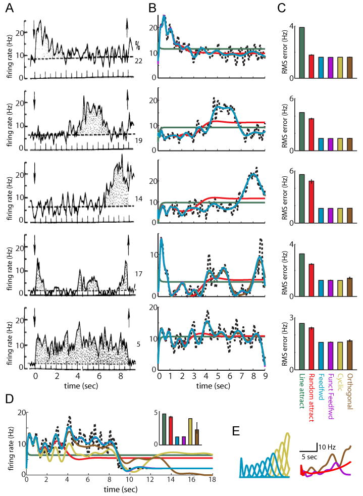
Generation of time-varying persistent neural activity by functionally feedforward versus positive-feedback models. (A) Trial-averaged, time-varying persistent neural activity of 5 neurons representing common classes of response observed in prefrontal cortical neurons during a visual working memory task (percentages of each class shown to the right of the plots). Adapted from Batuev (1994). (B) Fits to data in (A) attained by linearly summing the activities of neurons in networks with various connectivity patterns. Traces for the feedforward (cyan), functionally feedforward (purple), cyclic (mustard), and orthogonal (brown) networks overlap nearly exactly. For the functionally feedforward, Gaussian random (red), and random orthogonal networks, traces show the performance of the median of 100 randomly generated networks obeying the connectivity pattern. (C) Root mean squared error in the fits achieved by the median, 25^th and 75^th best performing network. (D) Fits to the persistent activity exhibited in the bottom panel of (A) when the networks were required to not only fit the delay period activity but also return to baseline activity at the end of the delay period. The functionally feedforward networks can stop responding at any time up to their maximal response duration by assigning zero readout weight to the later-occurring basis functions; the other networks cannot both fit the delay-period activity and return to baseline because they contain response modes that long outlast the delay period. (E) Examples of activity of individual neurons in the feedforward versus feedback-based networks when weights were increased by 2%. Left, feedforward versus cyclic networks. Right, functionally feedforward versus random attractor and random orthogonal networks. Exponential growth of the feedforward, but not feedback-based, networks is limited by the time taken for activity to propagate through the feedforward chain of activity patterns.

Generation of Constant-Rate Persistent Neural Activity

Line attractor networks have been widely used as models for the generation of persistent neural activity because, when properly tuned, these networks can sustain firing indefinitely (Fig. 7C). Furthermore, because these networks encode a single-dimensional quantity and do not respond persistently to inputs along other dimensions, they have the useful property that they can filter out irrelevant components of inputs. However, as has been widely noted, line attractor networks require a high degree of fine tuning in order to maintain persistence for long durations: too much feedback can lead to runaway growth of activity while too little feedback can be insufficient to overcome the intrinsic decay processes that set the neuronal integration time constant τ. For example, in order to produce persistent activity that is held constant to within ±5% for two seconds, a line attractor needs to be tuned to have an exponential decay time constant of 20 seconds. For a network of neurons with intrinsic time constants τ = 100 ms, this corresponds to tuning the network's weights to within 0.5% of the value required to sustain perfectly stable firing (Fig. 7B). Decreasing synaptic connection strengths more than this leads to an inability to sustain activity for the requisite 2 second period (Fig. 7A). Even worse, increasing connection strengths leads to runaway growth of activity (Fig. 7D).

A key reason why the line attractor requires such precise tuning is that its neurons exhibit identical activity patterns at times much beyond the time scale of the intrinsic time constant τ (Fig. 7A-D, middle panels). Therefore, a readout mechanism that sums the activities of such neurons will be constrained to exhibit this same activity pattern (lower panels). Stated another way, because all neurons behave in the same manner at long times, they can only accurately represent a single-dimensional temporal pattern. When the desired output pattern does not match this single-dimensional pattern, the network has no flexibility with which to adjust.

The feedforward network behaves very differently. Because it is feedforward, the duration ∼Nτ over which it can sustain persistent activity is strictly limited by the network size and the time constant of the feedforward stages. However, over this time scale it generates a diverse set of responses whose peaks are spaced evenly in time. Thus, in order to generate accurate persistent activity for two seconds, the network only needs to generate significant responses for two seconds (Fig. 7E). This is because the readout process can sum neuronal activities in a manner that compensates for imprecise tuning within the feedforward network (up to a point – in all simulations, readout weights were limited to a magnitude of 5 to avoid artificially good fits due to sums and differences of extremely large individual inputs; illustration of a network in which readout weights were not allowed to be adjusted to compensate for imprecise tuning within the feedforward network is shown in Supplemental Figure 3A). Furthermore, because the feedforward network runs out of stages after a time ∼Nτ, there is an inherent brake on runaway activity of neuronal responses at this time. Thus, the feedforward networks are more robust against weight increases that would cause instability in feedback-based networks (Fig. 7H).

The above example shows that, even for producing constant-rate persistent neural activity, the performance of the line attractor networks is less robust than that of the feedforward network. Nevertheless, a well-tuned line attractor can produce such activity and, in principle, can maintain such activity for limitless durations. Next, I consider an example of activity recorded during a working memory task in which the neuronal responses during a prolonged delay period do not exhibit constant activity but rather exhibit strong temporal variations that are consistently reproduced across trials (Fig. 8).

Generation of Time-Varying Persistent Neural Activity

Strongly temporally varying activity has been observed in neuronal recordings obtained during a variety of working memory related tasks (Baeg et al., 2003; Batuev, 1994; Batuev et al., 1979; Brody et al., 2003a; Deadwyler and Hampson, 2006; Pastalkova et al., 2008). In the study from which Figure 8A was taken, monkeys were required to remember a visual stimulus during a 9-second delay period and then, after a go-cue, press a button representing the remembered stimulus. Multielectrode recordings in prefrontal cortex revealed neurons that consistently (across trials) responded during particular portions of the delay period: early (top panel); middle (2^nd panel); late (3^rd panel); a mixture of early, middle, and/or late (4^th panel); or persistently throughout the delay period (bottom panel). Interestingly, only 5% of neurons in this study were found to exhibit tonic persistent activity throughout the delay period (Fig. 8A, percentages for each class of neurons are shown to the right).

The neuronal responses shown in Figure 8A cannot be described by the low-dimensional dynamics of the line attractor, in which all neurons exhibit similar responses at long times. When a 100 neuron line attractor with perfect tuning to give stable persistent firing was constructed, the neuronal responses of the network to a pulse of input all behaved in the same manner at times much beyond the intrinsic time constant τ (Fig. 9, green). Therefore, no matter how a readout mechanism summed these activities, they could not be fit to the time-varying activities seen in Figure 8A (Fig. 8B, dark green trace shows best fits). By contrast, the feedforward network fit the time-varying activity well (Fig. 8B, light blue) – this is because the feedforward basis functions have peaks spaced evenly over time, which provides a natural representation from which to construct a wide range of temporal activity patterns. A recurrently connected, but functionally feedforward network performed nearly identically to the architecturally feedforward network (Fig. 8B, purple trace not visible due to nearly perfect overlap with cyan feedforward trace). This suggests that the feedforward functionality of the network, not the feedforward network architecture, underlies the ability to fit these data.

Figure 9.

Activities of individual neurons for the networks tested in Figure 8. Left column, schematic of network connectivity for an unconnected network and the networks tested in Figure 8. Right column, example responses of 6 of the 100 neurons in each network. The unconnected network is shown to illustrate the intrinsic neuronal decay time constant τ=100 ms.

The good performance of the feedforward networks in fitting the time-varying persistent neural activity depended on two features. First, unlike the line attractor network, there were many independent modes of activity that could be used to fit the different time-varying responses. Second, a large number of these modes extended out for long time periods. Previous work in ‘liquid-state machine’ networks (Maass et al., 2002) has suggested how a network of randomly connected networks can be used to generate a diversity of temporal patterns, satisfying the first criterion above. However, the performance of such networks is best for time scales close to the intrinsic biophysical time scales of the individual neurons. To test if this was the case for the linear networks used in this study, a network was constructed with random connection strengths chosen from a Gaussian distribution (as in the study of Maass et al. (2002)) and the responses of this network to a pulse of input were fit to the data of Figure 8A. Typically the activity of the neurons in such networks either decayed on a time scale set by the intrinsic time constant τ or, if connections were too strong, exhibited runaway growth of activity (data not shown). Even when the mean and variance of the Gaussian distribution were tuned to give the network a persistent mode of activity, the activity observed was low-dimensional at long time scales (as in the line attractor network) and did not capture time-varying activity after the first few seconds (Fig. 8B, red lines give best fits; example neuronal firing rates in response to a pulse of input for this and the other networks in this study are shown in Figure 9).

The above example suggests that randomly connecting neurons into a network does not lead to many modes of activity that persist far beyond the intrinsic time constant τ. Rather, it suggests that special network architectures may be required to generate a diversity of temporal responses at long time scales. The feedforward and functionally feedforward networks provide two examples that differ sharply from traditional models of persistent neural activity based on positive feedback. For discussion of other networks (cyclic and random orthogonal networks, Figs. 8, 9) that were found to fit the data well, and their relationship to the feedforward networks focused on here, see the Discussion. For a complementary approach (pseudospectral analysis) to analyzing the functionally feedforward networks, see the Supplemental Methods.

Discussion

Traditional neural network models of short-term memory and persistent neural activity have assumed that positive feedback is required for the generation of long-lasting activity in the absence of a stimulus. This study has shown how graded persistent activity and temporal integration can be generated even by networks that entirely lack positive feedback. Thus, while it is traditional to search for positive feedback loops as a substrate for long-lasting persistent neural activity, such feedback loops are not required. Rather, feedback and feedforward mechanisms may operate in tandem with, for example, feedback interactions being used to set the time scales τ with which the feedforward stages of a network filter their inputs.

Feedforward interactions were shown to occur not only in architecturally feedforward networks but also in recurrent networks that can act as “feedforward networks in disguise” by propagating activity through a feedforward cascade of activity patterns. Such feedforward interactions could not be identified by traditional eigenvector-based methodologies for analyzing recurrent networks because eigenvectors only identify feedback interactions. Using the Schur decomposition, additional feedforward interactions were identified, and it was shown that the generic behavior of recurrent networks is to contain both feedforward and feedback interactions.

Comparison of functionally feedforward and feedback networks

The performance of feedforward and feedback-based networks in fitting constant-rate and time-varying persistent activity were compared in order to ascertain their relative advantages and disadvantages. These comparisons revealed two features that determined network performance: (1) the number of modes of network activity present at a given time scale, and (2) the susceptibility of the network to instability. At one extreme are the line attractors, with only a single persistent mode of activity. These networks are the most efficient in terms of number of required neurons – a line attractor can be constructed from a single neuron connected with an autapse onto itself (Seung et al., 2000). Furthermore, input components along non-persistent modes decay away quickly, which can be useful for filtering out irrelevant inputs when only a single-dimensional quantity needs to be stored. However, due to their one-dimensional temporal dynamics, such networks can only be used to fit a single stereotyped temporal activity pattern such as constant-rate persistent activity. Furthermore, even to maintain graded constant-rate persistent activity to a high degree of accuracy over a fixed period of time (e.g. 2 seconds in Figure 7), these networks needed to be tuned to have exponential decay over a much longer time period.

With increased numbers of neurons, the networks can generate more independent modes of activity – generically N modes of activity for a network of N neurons. However, unless the networks are specially constructed, the duration of most activity modes will be set by the time scale τ of the intrinsic biophysics of the neurons in the network and will contain few, if any persistent modes of activity. This may explain why previous studies of temporal processing by networks with random connectivities, such as those used to model temporal intervals (Buonomano, 2000; Karmarkar and Buonomano, 2007) and temporal classification (Maass et al., 2002), were limited in applicability to time intervals on the order of 1 second (on the order of the largest biophysical time constant in the networks).

The feedforward networks can generate a wide variety of temporal activity patterns because their responses are built from basis functions g_n that form a natural representation of time. An identical representation of time over the time scale of the delay period could be generated by a recurrent network with a “cyclic” architecture in which the last of the chain of neurons of the feedforward network connects back onto the first (Fig. 9, mustard lines), so that activity is identical to a feedforward network during the first time around the cycle. This cyclic network and heterogeneously connected generalizations of it (White et al., 2004) produced nearly identical fits to the feedforward networks for the time-varying data of Figure 8 (Fig. 8B, mustard and brown lines). However, at longer times, activity in the orthogonal networks persisted whereas activity in the feedforward network rapidly decayed to baseline levels (Fig. 8D). Thus, the feedforward networks have the disadvantage of a limited memory time span but the possible advantages of a built-in reset and clearing of their memory buffer (Fig. 8D) and robustness against runaway growth (Fig. 8E).

Comparison to experiment and further studies

An open experimental question is when a system will generate high-dimensional versus low-dimensional persistent activity patterns. Batuev (1994) observed high-dimensional, time-varying activity in prefrontal, but not parietal cortex, consistent with a recent study of persistent activity in lateral intraparietal cortex that found rapid decay to a single eigenmode of activity during decision-making tasks (Ganguli et al., 2008). Peaks in firing that occur at different times during the delay period for different neurons have also been recorded in other prefrontal working memory experiments (Baeg et al., 2003), as well as in the hippocampus and subiculum (Deadwyler and Hampson, 2006; Pastalkova et al., 2008). In the cat oculomotor neural integrator, neurons have been reported to exhibit a progressive lengthening of the time constant of integration (qualitatively similar to that shown in Figure 2B) with decreasing distance from the motor output nuclei, and these data have been suggested to reflect a primarily feedforward cascade of processing (Delgado-Garcia et al., 1989; Escudero et al., 1992). Further experimental work will be needed to probe how persistent neural activity depends upon task demands and brain region, as well as to design new working memory tasks with more complex temporal processing requirements.

Theoretical work can complement such experiments by testing how feedforward or feedback-based architectures may emerge from physiologically-based learning rules. Previous study of working memory networks that maintain a graded representation of a memorized stimulus have suggested that a key component of such learning rules may be homeostatic plasticity mechanisms (Turrigiano et al., 1998) that keep neuronal firing rates from growing too large or too small (Renart et al., 2003). Application of a homeostatic learning rule to a simple feedforward chain of neurons did produce a working feedforward integrator (Supplemental Fig. 3), but further study is needed with more general network architectures.

This study has focused on linear networks whose response amplitude varies linearly with the input. If graded responses to inputs are not a feature of the networks being modeled, then adding bistable or digital processes to the neurons (Camperi and Wang, 1998; Goldman et al., 2003; Koulakov et al., 2002) could provide robustness by preventing small increases or decreases in synaptic weights from causing a cascading increase or decrease in responses as activity propagates through the network. Digitization of responses is a hallmark of models of sequence processing that propagate activity through a sequence of metastable states (Hopfield, 1982; Kleinfeld, 1986; Sompolinsky and Kanter, 1986; Rabinovich et al., 2008) and, when accomplished through an intrinsic bursting mechanism, has been suggested to underlie the robustness of temporal sequence generation in birdsong nucleus HVC (Jin et al., 2007).

A powerful advantage of the feedforward networks discussed here is their flexibility to be extended to more temporally complex tasks than generating constant-rate persistent activity or linearly accumulating an input. Unlike line attractor models, the feedforward integrator's output is generated as a combination of basis functions that are each peaked around a particular time. These basis functions could serve as a neural representation of time during a working memory period, or, when combined with unequal weights, be used to generate complex temporal sequences from a triggering pulse of input. Previous work in signal processing has shown that the basis functions g_n, or similar ones, can be combined to form complex filters for use in a host of temporal sequence processing tasks ranging from speech recognition to EEG analysis (Principe et al., 1993; Tank and Hopfield, 1987). Thus, placing persistent activity in the more general context of temporal processing provides a unifying framework in which to view temporal sequence recognition, generation, and accumulation in memory.

Experimental Procedures

Architecturally feedforward networks

Networks were defined by the linear network equations

$$\tau \frac{d{r}_i}{dt}=-r_i+\sum _j{w}_{ij}{r}_j+a_{i}x(t)$$ (2)

where r_i represents the average activity of unit i, w_ij is the connection strength from unit j to unit i, x(t) represents the external input to be integrated, and a_i represents the strength of the external input to unit i. The architecturally feedforward networks were defined by having w_ij=0 for i ≤ j.

The dynamics of the rearranged feedforward network with equivalent output (Fig. 1A, right) is defined by the equations

$$\begin{array}{l}\tau \frac{d{R}_n}{dt}=-R_n+R_{n-1},1\le n\le (N-1)\hfill \\ \tau \frac{d{r}_{\text{out}}}{dt}=-r_{\text{out}}+\sum _{n=0}^{N-1}{W}_i{R}_i\hfill \end{array}$$ (3)

where R₀=x(t) represents the external input and R_n for n≥1 represents the activity of the n^th stage. W_n represents the summed weight of all paths that reach the output stage through n intermediate stages, where the weight of a path equals the product of a_i and all synaptic weights w_ij connecting the neurons along this path. For the optimally fit summed outputs (Figs. 1, 2, 6, 7) and fits to time-varying delay period activity (Fig. 8), readout weights were constrained to |W_n|≤5 to prevent the network from artificially using differences of large weights to attain perfect fits. Network performance was highly insensitive to the exact constraint used as long as the maximum allowed magnitude of weights was at least a few to several times greater than 1, depending on the particular simulation.

For the network of Figure 2A, clusters of recurrently connected neurons with intrinsic decay time constants of 100 ms were connected to each other with uniform excitatory weights w_rec=0.4 to produce stages that collectively had a time constant τ = 500 ms. Each neuron also projected forward with weights w_ff=0.2/3 to each neuron in the following cluster. When a pulse of input was applied to each neuron in the first cluster, the neurons in this and subsequent clusters behaved identically to neurons in a simpler network consisting of a chain of neurons with biophysical time constant τ (Fig. 2A, effective network).

For the feedforward network of Figure 2B, all weights w_ij=0 except for those projecting forward to the neighboring stage, which were set to 1. The response of each stage of this network can be accounted for by delineating all possible pathways from the external input to this stage. The first stage receives only direct input; therefore its response corresponds to filtering the input once and equals the first temporal basis function. The second stage receives both direct input and input that traversed through the first stage; thus, its response equals a sum of the first two basis functions. The i^th stage receives direct input plus input that arrived directly at each of the earlier stages; its response therefore equals a sum of the first i basis functions. This explains why the final stage's response is identical to the equally weighted sum shown in Figure 2A (bottom, black trace).

The network of Figure 2C consisted of N=20 stages (columns in Fig. 2C) that each contained 20 units. Feedforward connections were chosen randomly with a 10% connection probability for units in neighbouring stages and a 0.2% probability for units in further separated stages. The pulse input had a 50% probability of connecting to units in the first stage and a 5% probability of connecting to units in all other stages. Weights between connected units equalled 10.

Eigenvector and Schur decompositions

The eigenvector and Schur decompositions each decompose a network into a set of activity patterns (states, Fig. 5B,C) that interact through a matrix that is simpler in form than the original connectivity matrix (Fig. 5A-C, interactions). Eigenvector analysis finds non-interacting components by “diagonalizing” the connectivity matrix w into the form w = VDV^-1, where D is a diagonal matrix (Fig. 5B, bottom) whose elements are the eigenvalues λ, and V is a matrix whose columns contain the eigenvector patterns of activity (states, Fig. 5B top). One can conceptualize such a transformation as a change of the coordinate axes from the cardinal axes x₁, x₂,… that represent the firing activity of neurons 1,2,… to a new set of axes that point along the directions of the eigenvectors. The matrix V^-1 transforms the neuronal activities x_i into their components along the new eigenvector axes. The matrix D characterizes the effect of the network's interactions on each of these components – because it is diagonal, the component patterns interact only with themselves and the eigenvalues represent the strength of these self-feedback interactions. The matrix V transforms back from the eigenvector coordinate system to the actual neuronal activities x_i.

Eigenvectors are not generally orthogonal to one another. The Schur decomposition (Horn and Johnson, 1985) finds a set of orthogonal patterns of activity (Fig. 5C, top; Fig. 5D, right) that have both self-feedback interactions given by the same eigenvalues as in the eigenvector decomposition and also feedforward interactions (Fig. 5C, bottom). Mathematically, the Schur decomposition of a matrix w is given by w = UTU^-1, where U is a matrix whose columns contain the orthogonal Schur mode patterns of activity and T is a triangular matrix that contains the eigenvalues along the diagonal and the feedforward interactions between states in the lower (or upper, depending on convention) triangular elements. Note that the exact choice of U and T is not unique although the diagonal entries of T always equal the eigenvalues and the off-diagonal entries always sum to the same fixed value for a given matrix w. For all functionally feedforward networks in this paper, the weight matrix w was constructed by running the Schur decomposition “in reverse”: A set of N orthogonal patterns were generated randomly by applying a Gram-Schmidt orthogonalization procedure to a set of N randomly generated vectors, and the resulting patterns were assembled into the columns of a matrix U. Next, a feedforward matrix T was defined to describe the interactions between these patterns and then multiplied on the left by U and on the right by U^-1. For the feedforward chain, T_ij =1 for i =j+1 and 0 otherwise. Because the vectors represented by the columns of U are orthogonal, they can be considered to be rotated versions of the Cartesian axes x₁, x₂, x₃ and the matrix w corresponds to a “rotated” version of the feedforward matrix T, as depicted in Figure 3. A key property of any coordinate rotation is that it preserves the eigenvalue spectrum of the rotated matrix. Therefore, as in the feedforward matrices T from which they were constructed, all eigenvalues of the functionally feedforward matrices equal zero and the eigenvalue analysis fails to predict the long time scales generated by these networks (however, such long time scales are predicted by a pseudoeigenvalue analysis – see the Supplemental Methods).

Detailed description of the connectivity matrices of the networks tested in Figures 7 and 8, as well as their eigenvalue and pseudoeigenvalue spectra (Supplemental Figs. 1 and 2), is given in the Supplemental Methods. A description of the homeostatic learning rule used to generate Supplemental Figure 3B is also included in the Supplemental Methods.

References

- Baeg EH, Kim YB, Huh K, Mook-Jung I, Kim HT, Jung MW. Dynamics of population code for working memory in the prefrontal cortex. Neuron. 2003;40:177–188. doi: 10.1016/s0896-6273(03)00597-x. [DOI] [PubMed] [Google Scholar]
- Batuev AS. Two neuronal systems involved in short-term spatial memory in monkeys. Acta Neurobiol Exp (Wars) 1994;54:335–344. [PubMed] [Google Scholar]
- Batuev AS, Pirogov AA, Orlov AA. Unit activity of the prefrontal cortex during delayed alternation performance in monkey. Acta Physiol Acad Sci Hung. 1979;53:345–353. [PubMed] [Google Scholar]
- Brody CD, Hernandez A, Zainos A, Romo R. Timing and neural encoding of somatosensory parametric working memory in macaque prefrontal cortex. Cereb Cortex. 2003a;13:1196–1207. doi: 10.1093/cercor/bhg100. [DOI] [PubMed] [Google Scholar]
- Brody CD, Romo R, Kepecs A. Basic mechanisms for graded persistent activity: discrete attractors, continuous attractors, and dynamic representations. Curr Opin Neurobiol. 2003b;13:204–211. doi: 10.1016/s0959-4388(03)00050-3. [DOI] [PubMed] [Google Scholar]
- Buonomano DV. Decoding temporal information: A model based on short-term synaptic plasticity. J Neurosci. 2000;20:1129–1141. doi: 10.1523/JNEUROSCI.20-03-01129.2000. [DOI] [PMC free article] [PubMed] [Google Scholar]
- Camperi M, Wang XJ. A model of visuospatial working memory in prefrontal cortex: recurrent network and cellular bistability. J Comput Neurosci. 1998;5:383–405. doi: 10.1023/a:1008837311948. [DOI] [PubMed] [Google Scholar]
- Deadwyler SA, Hampson RE. Temporal coupling between subicular and hippocampal neurons underlies retention of trial-specific events. Behav Brain Res. 2006;174:272–280. doi: 10.1016/j.bbr.2006.05.038. [DOI] [PubMed] [Google Scholar]
- Delgado-Garcia JM, Vidal PP, Gomez C, Berthoz A. A neurophysiological study of prepositus hypoglossi neurons projecting to oculomotor and preoculomotor nuclei in the alert cat. Neuroscience. 1989;29:291–307. doi: 10.1016/0306-4522(89)90058-4. [DOI] [PubMed] [Google Scholar]
- Durstewitz D, Seamans JK, Sejnowski TJ. Neurocomputational models of working memory. Nat Neurosci. 2000;(3 Suppl):1184–1191. doi: 10.1038/81460. [DOI] [PubMed] [Google Scholar]
- Escudero M, de la Cruz RR, Delgado-Garcia JM. A physiological study of vestibular and prepositus hypoglossi neurones projecting to the abducens nucleus in the alert cat. J Physiol. 1992;458:539–560. doi: 10.1113/jphysiol.1992.sp019433. [DOI] [PMC free article] [PubMed] [Google Scholar]
- Ganguli S, Huh D, Sompolinsky H. Memory traces in dynamical systems. Proc Natl Acad Sci U S A. 2008;105:18970–18975. doi: 10.1073/pnas.0804451105. [DOI] [PMC free article] [PubMed] [Google Scholar]
- Goldman MS, Levine JH, Major G, Tank DW, Seung HS. Robust persistent neural activity in a model integrator with multiple hysteretic dendrites per neuron. Cereb Cortex. 2003;13:1185–1195. doi: 10.1093/cercor/bhg095. [DOI] [PubMed] [Google Scholar]
- Hopfield JJ. Neural networks and physical systems with emergent collective computational abilities. Proc Natl Acad Sci U S A. 1982;79:2554–2558. doi: 10.1073/pnas.79.8.2554. [DOI] [PMC free article] [PubMed] [Google Scholar]
- Horn RA, Johnson CR. Matrix Analysis. Cambridge, UK: Cambridge University Press; 1985. [Google Scholar]
- Huk AC, Shadlen MN. Neural activity in macaque parietal cortex reflects temporal integration of visual motion signals during perceptual decision making. J Neurosci. 2005;25:10420–10436. doi: 10.1523/JNEUROSCI.4684-04.2005. [DOI] [PMC free article] [PubMed] [Google Scholar]
- Jin DZ, Ramazanoglu FM, Seung HS. Intrinsic bursting enhances the robustness of a neural network model of sequence generation by avian brain area HVC. J Comput Neurosci. 2007;23:283–299. doi: 10.1007/s10827-007-0032-z. [DOI] [PubMed] [Google Scholar]
- Karmarkar UR, Buonomano DV. Timing in the absence of clocks: encoding time in neural network states. Neuron. 2007;53:427–438. doi: 10.1016/j.neuron.2007.01.006. [DOI] [PMC free article] [PubMed] [Google Scholar]
- Kleinfeld D. Sequential state generation by model neural networks. Proc Natl Acad Sci U S A. 1986;83:9469–9473. doi: 10.1073/pnas.83.24.9469. [DOI] [PMC free article] [PubMed] [Google Scholar]
- Koulakov AA, Raghavachari S, Kepecs A, Lisman JE. Model for a robust neural integrator. Nat Neurosci. 2002;5:775–782. doi: 10.1038/nn893. [DOI] [PubMed] [Google Scholar]
- Maass W, Natschlager T, Markram H. Real-time computing without stable states: a new framework for neural computation based on perturbations. Neural Comput. 2002;14:2531–2560. doi: 10.1162/089976602760407955. [DOI] [PubMed] [Google Scholar]
- Major G, Tank D. Persistent neural activity: prevalence and mechanisms. Curr Opin Neurobiol. 2004;14:675–684. doi: 10.1016/j.conb.2004.10.017. [DOI] [PubMed] [Google Scholar]
- Pastalkova E, Itskov V, Amarasingham A, Buzsaki G. Internally generated cell assembly sequences in the rat hippocampus. Science. 2008;321:1322–1327. doi: 10.1126/science.1159775. [DOI] [PMC free article] [PubMed] [Google Scholar]
- Principe JC, De Vries B, De Oliveira PG. The gamma-filter - a new class of adaptive IIR filters with restricted feedback. IEEE Trans Signal Processing. 1993;41:649–656. [Google Scholar]
- Rabinovich M, Huerta R, Laurent G. Transient dynamics for neural processing. Science. 2008;321:48–50. doi: 10.1126/science.1155564. [DOI] [PubMed] [Google Scholar]
- Renart A, Song P, Wang XJ. Robust spatial working memory through homeostatic synaptic scaling in heterogeneous cortical networks. Neuron. 2003;38:473–485. doi: 10.1016/s0896-6273(03)00255-1. [DOI] [PubMed] [Google Scholar]
- Robinson DA. Integrating with neurons. Annu Rev Neurosci. 1989;12:33–45. doi: 10.1146/annurev.ne.12.030189.000341. [DOI] [PubMed] [Google Scholar]
- Seung HS, Lee DD, Reis BY, Tank DW. The autapse: a simple illustration of short-term analog memory storage by tuned synaptic feedback. J Comput Neurosci. 2000;9:171–185. doi: 10.1023/a:1008971908649. [DOI] [PubMed] [Google Scholar]
- Sompolinsky H, Kanter II. Temporal association in asymmetric neural networks. Phys Rev Lett. 1986;57:2861–2864. doi: 10.1103/PhysRevLett.57.2861. [DOI] [PubMed] [Google Scholar]
- Tank DW, Hopfield JJ. Neural computation by concentrating information in time. Proc Natl Acad Sci USA. 1987;84:1896–1900. doi: 10.1073/pnas.84.7.1896. [DOI] [PMC free article] [PubMed] [Google Scholar]
- Trefethen LN, Embree M. Spectra and pseudospectra: The behavior of nonnormal matrices and operators. Princeton, NJ: Princeton University Press; 2005. [Google Scholar]
- Turrigiano GG, Leslie KR, Desai NS, Rutherford LC, Nelson SB. Activity-dependent scaling of quantal amplitude in neocortical neurons. Nature. 1998;391:892–896. doi: 10.1038/36103. [DOI] [PubMed] [Google Scholar]
- Wang XJ. Synaptic reverberation underlying mnemonic persistent activity. Trends Neurosci. 2001;24:455–463. doi: 10.1016/s0166-2236(00)01868-3. [DOI] [PubMed] [Google Scholar]
- White OL, Lee DD, Sompolinsky H. Short-term memory in orthogonal neural networks. Phys Rev Lett. 2004;92:148102. doi: 10.1103/PhysRevLett.92.148102. [DOI] [PubMed] [Google Scholar]
Associated Data
This section collects any data citations, data availability statements, or supplementary materials included in this article.