Factors Affecting Accuracy From Genomic Selection in Populations Derived From Multiple Inbred Lines: A Barley Case Study

Abstract

We compared the accuracies of four genomic-selection prediction methods as affected by marker density, level of linkage disequilibrium (LD), quantitative trait locus (QTL) number, sample size, and level of replication in populations generated from multiple inbred lines. Marker data on 42 two-row spring barley inbred lines were used to simulate high and low LD populations from multiple inbred line crosses: the first included many small full-sib families and the second was derived from five generations of random mating. True breeding values (TBV) were simulated on the basis of 20 or 80 additive QTL. Methods used to derive genomic estimated breeding values (GEBV) were random regression best linear unbiased prediction (RR–BLUP), Bayes-B, a Bayesian shrinkage regression method, and BLUP from a mixed model analysis using a relationship matrix calculated from marker data. Using the best methods, accuracies of GEBV were comparable to accuracies from phenotype for predicting TBV without requiring the time and expense of field evaluation. We identified a trade-off between a method's ability to capture marker-QTL LD vs. marker-based relatedness of individuals. The Bayesian shrinkage regression method primarily captured LD, the BLUP methods captured relationships, while Bayes-B captured both. Under most of the study scenarios, mixed-model analysis using a marker-derived relationship matrix (BLUP) was more accurate than methods that directly estimated marker effects, suggesting that relationship information was more valuable than LD information. When markers were in strong LD with large-effect QTL, or when predictions were made on individuals several generations removed from the training data set, however, the ranking of method performance was reversed and BLUP had the lowest accuracy.

WITH the advent of cheap and high-density array-based DNA marker technologies, genomewide dense molecular markers are becoming available for livestock and crop species. As examples, cattle geneticists have genotyping systems that provide >50,000 single nucleotide polymorphisms (SNP; VanRaden et al. 2009); the U. S. Department of Agriculture-sponsored Barley Coordinated Agricultural Project (CAP) is developing 3000 informative SNP to be scored on 3840 elite U. S. breeding lines. Meuwissen et al. (2001) developed a method called “genomic selection” to predict breeding values using precisely this kind of genomewide dense marker data. Marker effects are first estimated on a training data set with marker genotypes and trait phenotypes. Breeding value can then be predicted for any genotyped individual in the population using the marker-effect estimates. Simulation studies have shown that genomic selection can lead to high correlations between predicted and true breeding value over several generations without repeated phenotyping (Meuwissen et al. 2001; Habier et al. 2007). Therefore, genomic selection can result in lower costs and increased rates of genetic gain.

Several statistical methods have been proposed for analysis of the training data for genomic selection. Meuwissen et al. (2001) and Habier et al. (2007) compared least squares, random-regression best linear unbiased prediction (RR–BLUP) and Bayesian methods (Bayes-A and Bayes-B). Xu (2003) proposed a Bayesian shrinkage approach for quantitative trait locus (QTL) detection on the basis of the genomic-selection idea (Meuwissen et al. 2001). ter Braak et al. (2005) provided modifications to the Xu (2003) model to ensure proper posterior distributions-of-effect estimates and to better estimate QTL locations. We can regard these Bayesian shrinkage regression methods as another form of genomic selection when using them to predict breeding values. In previous work, these genomic-selection prediction methods have predominantly been compared under a specific simulation scenario such that their relative strengths under different conditions of linkage disequilibrium (LD), marker density, training data set size, and distribution of QTL effects are not known. Furthermore, genomic selection was pioneered in animal breeding systems and few studies have considered plant breeding systems. Indeed, genomic selection in plants has been studied only for populations derived from crosses of biparental lines (Bernardo and Yu 2007; Piyasatian et al. 2007; Zhong and Jannink 2007). The extent and nature of LD in such populations, however, will be quite different from populations with many founders in mutation-drift-recombination equilibrium.

Plant breeding populations have special characteristics relative to animal breeding populations. In particular, plant breeders often work with full-sib families created from crosses of inbred parents that vary in size, whereas half-sib families from non-inbred parents are more typical in animal breeding. Extensive LD will arise within each family but, given differing linkage phases across families, LD across a large set of families should represent the underlying population-wide LD. In typical plant-breeding practice, enough lines from a germplasm pool will have been sampled such that associations with a dense marker set should be consistent population-wide, which would be particularly useful for association mapping or marker-assisted selection (MAS) (Yu et al. 2008). Another characteristic of plant breeding is that the use of inbred lines is common and breeders usually have the ability to replicate individual genotypes over space and time and, by averaging across replicates, can thus obtain very accurate phenotypic measurements for a quantitative trait. Given a fixed amount of resources, breeders have the option to evaluate more individuals with lower accuracy or fewer individuals with higher accuracy. These characteristics might affect how genomic selection should be carried out in crops relative to livestock.

Barley offers an excellent public-sector model for crops because the Barley CAP and its partners have generated >4500 SNP from expressed sequence tags. These SNP have been scored on the “Barley CAP core,” a set of 102 inbred barley lines primarily of U. S. origin. We used this data set as a starting point to test genomic selection for levels and structures of LD that are realistic for a self-pollinating crop. Here, we report on the relative performance of alternate genomic-selection prediction methods under different conditions of marker density, QTL effect distribution, and training data set size using mating schemes that affected the extent of LD. We also assessed the adequacy of the marker density that is currently available for barley for genomic selection, contrasting the accuracies of genomic estimated breeding values (GEBV) with those that might be obtained from phenotypic information.

MATERIALS AND METHODS

Overview:

An ideal evaluation of genomic-selection estimation methods would require large data sets of individuals with known breeding values scored at high marker density. In the absence of such data sets, we simulated them realistically on the basis of actual barley marker data. These data encapsulate actual LD structure upon which we can impose a genetic model to obtain phenotypes and true breeding values. Simulated mating designs allow generation of samples of different sizes and levels of LD, enabling us to explore a broad range of scenarios. In the following, we describe the original Barley CAP core data set, the assumed genetic model, the mating designs used to generate samples, and, finally, the genomic-selection prediction models that were evaluated.

Germplasm and genetic map:

To avoid excessive population structure due to the historical separation between six- and two-row barley, we worked only with data from 42 two-row spring barley lines (see supporting information, Table S1). The 1933-locus, 1279-cM map constructed by Peter Szucs and Patrick Hayes on the Oregon Wolfe Barley (OWB) population (http://www.barleycap.org/) was used as the reference map. This map contains Diversity Array Technology (DArT) markers, SNP, and classical markers (e.g., simple sequence repeat and restriction enzyme fragment polymorphism markers). The SNP genotypes were obtained from two Illumina GoldenGate assays. One assay was described in Rostoks et al. (2006) and the other was developed by similar methods (T. J. Close, personal communication). Map positions of SNP and classical markers based on other mapping populations (T. J. Close, personal communication) were obtained from HarvEST: Barley 1.64 (http://harvest.ucr.edu/). A consensus map of DArT and classical markers was obtained from Wenzl et al. (2006). The following expedient approach was used to merge these maps. First, common markers between the OWB and each of the other two maps were identified. Per chromosome, there were on average 77 (range: 65–97) and 69 (range: 32–94) markers in common between the OWB and the SNP and DArT maps, respectively. The OWB map positions were then regressed on SNP map positions and on DArT map positions to project the SNP and DArT maps onto OWB-predicted positions. A marker's final linkage map position was estimated as the mean of all available OWB or OWB-predicted positions. Only markers that had a minor allele frequency >0.1 across the 42 two-row spring barley lines were used. This criterion resulted in the selection of 1605 markers. Markers were then chosen so that they were at least 0.2 or 0.75 cM apart, resulting in dense and sparse settings of 1040 and 575 markers, respectively. In both settings, there were 19 marker gaps >5 cM. All markers were biallelic. Given the low rate of missing marker data (1.7%), missing marker genotypes were randomly assigned according to their population allele frequency.

Genetic model:

All loci were biallelic with inbred genotypes coded as 0 or 1. The number of segregating QTL affecting the trait was set at either 20 or 80. QTL were simulated by randomly drawing positions on the genetic map and assigning the closest marker among the 1040 and 575 to be a QTL. One marker allele was randomly chosen to have a positive effect and the other to have a negative effect on the simulated trait. QTL effect sizes were scaled according to the allele frequencies to obtain variances that followed a geometric series (Lande and Thompson 1990). The breeding value of a line was the sum of the effects of the QTL alleles that it carried. To obtain the phenotype, we added a normal error deviate with variance calculated to achieve the desired heritability.

Mating designs:

Using the 42 lines as a founder pool, we simulated four mating designs by pairing inbred lines, generating gametes according to Mendelian inheritance assuming no crossover interference, and then by doubling the gametes to create doubled haploid (DH) lines. These mating designs, which are described in detail in the following and are summarized in Table 1, produced the training data sets that were analyzed by genomic-selection methods to predict breeding values of individuals in testing data sets. Regardless of the mating design used to generate the training data set, the testing data set was produced by one or four generations of 500 random crosses between the DH lines of the training data, each with one progeny.

TABLE 1.

Mating designs used to simulate training data sets from 42 inbred founders

	Design 1	Design 2	Design 3	Design 4	Design 1–1000	Design 2–1000
Generations of mating	1	5	1	5	1	5
Mating structure	Round	Random	Round	Random	Round	Random
No. of families	42	500	42	168	42	1000
No. of DH per family	12	1	4	1	12	1
No. of lines	504	500	168	168	1008	1000
Heritability	0.4	0.4	0.67	0.67	0.4	0.4

Design 1:

Training data sets of 42 families of 12 DHs (504 DHs in total) were generated using a single round-robin design (Verhoeven et al. 2006); i.e., the lines were first randomly ordered and then crossed as follows: line 1 × line 2, line 2 × line 3, …, line 42 × line 1. To evaluate the effect of increasing the training data set size, we also generated design 1–1000 data sets in which each family contained 24 DHs, resulting in 1008 lines.

Design 2:

Training data sets of 500 double haploids with lower long-range LD than in design 1 were derived after randomly mating the original 42 lines for five generations. The population size during random mating was 200 individuals, and 500 DHs were derived at random from the last generation. Design 2–1000 data sets that contained 1000 DHs were also created. The environmental variance for these designs was set such that the heritability was 0.4 for the original 42 lines.

Designs 3 and 4:

Designs 3 and 4 were similar to designs 1 and 2, respectively, but had one-third as many DHs. Assuming a fixed number of plots to grow plants, this would allow for increased replication. A heritability of 0.67 was used to simulate phenotypes for each DH, given that we had one-third the number of DH lines and therefore could afford three times more replicates relative to designs 1 and 2.

Linkage disequilibrium measures:

Markers with minor allele frequency >0.2 in the Barley CAP core were used to estimate the extent of LD between all pairs of markers within 100 cM in all chromosomes. The LD was computed as the squared correlation between alleles at two markers: 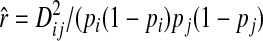(Hill and Robertson 1968), where 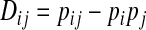and p_ij, p_i, and p_j are the frequencies of haplotype ij and allele i at one locus and allele j at the other locus.

Statistical models:

Four genomic-selection prediction methods were used for analysis of each training data set. Two were as described by Meuwissen et al. (2001): RR–BLUP and Bayes-B. RR–BLUP assumed that each marker had variance equal to V_G/M, where V_G is the genetic variance and M is the number of markers. In the Bayes-B approach, the prior for the proportion of markers associated with zero phenotypic variance, π, was assumed known. We evaluated two values, π = (M − 80)/M (denoted Bayes-B1) and π = (M − 150)/M (denoted Bayes-B2). Other prior hyperparameters for marker variance components were the same between Bayes-B1 and Bayes-B2 and were as given in Meuwissen et al. (2001). The third statistical method was based on ter Braak et al.'s (2005) improvements to the Bayesian shrinkage regression method developed by Xu (2003), which shrinks small effects toward zero (denoted “Xu2003”). In the fourth method, markers were used only to estimate the relationship between lines. First, a marker-based relationship matrix, 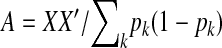, was calculated, where X is the DH line by marker matrix of marker scores, the summation is over all markers, and p_k is the allele frequency at marker k in the training data set (Habier et al. 2007; VanRaden and Tooker 2007). To ensure a positive definite matrix, 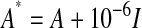was used in calculations (I is the identity matrix). The heritability used to solve the mixed model equations was set at the simulated heritability. To obtain breeding value estimates for the testing data set, A was calculated across the DH lines from both training and testing sets. Because this method uses an estimate of the realized A matrix, we called it the RA–BLUP method.

In some cases, although the QTL were not identified, their genotypes were included along with all other markers in the analysis. We contrast these “observed” QTL cases to more typical “unobserved” QTL cases. For each mating design and marker density scenario, 30–50 replicates were simulated and analyzed using the four methods. After each analysis, the predicted breeding values of the testing data set sample were correlated with their known true breeding values. This prediction accuracy was used as the performance criterion for the methods.

RESULTS

Extent of LD in two-row barley founders:

Despite avoiding structure due to the division between two- and six-row barley, many instances of long-range LD remained among the 42 founders (Figure 1A), in agreement with previous studies in barley (Kraakman et al. 2004; Rostoks et al. 2006). Even though high long-range LD occurred, LD at short range was low, averaging about = 0.25 for markers <0.25 cM apart. The single round-robin mating of design 1 removed high LD ( > 0.4) at distances >30 cM (Figure 1B), although moderate LD ( > 0.2) still occasionally extended to 100 cM. After the five rounds of random mating as in design 2, moderate LD occurred only up to distances of ∼15 cM (Figure 1C). Design 2 also eliminated long-distance LD greater than an of 0.1. Thus, as expected, recombination in designs 1 and 2 greatly reduced long-distance LD but had little effect on LD at distances <2 cM (Figure 1). If we assume that LD between marker pairs approximates LD between markers and QTL, the marker density of ∼1/cM available for this study would often lead QTL to be only in low LD with any marker: for example, for QTL within 0.5 cM of a marker, the was >0.6 only about one-fourth of the time among the original 42 lines.

Figure 1.—

Decline of LD as measured by against distance in centimorgans for all markers with minor allele frequency >0.2 (858 markers in total). (A–C) in the original 42 lines, design 1 and design 2, respectively. Gray lines are smoothed running averages.

Prediction accuracy using genomic selection:

Prediction accuracy—that is, the correlation between the breeding values predicted by genomic selection and the true values known from simulation—ranged from 0.35 to 0.85 across the different scenarios analyzed (Figure 2). When the causal SNPs were observed and QTL effects were large, the Xu2003 method gave the best and the RR–BLUP the worst predictions (Figure 2B for 20 QTL). The performance of the Xu2003 method, however, declined sharply either when QTL effects were small (Figure 2B for 80 QTL) or when QTL genotypes were not observed (Figure 2, A, C, and D). In almost all scenarios, Bayes-B2, with a higher prior proportion of non-zero markers, outperformed Bayes-B1 (Figure 2); they performed equally only when there were 20 QTL and the causal SNPs were observed (Figure 2B). In almost all scenarios, predictions were better when LD was high (designs 1 and 3, Figure 2) than when it was low (designs 2 and 4, Figure 2), the sole exception being the scenario with 20 observed QTL. Predictions were more accurate in the dense than in the sparse marker scenarios (Figure 2A vs. Figure 2C), an effect that was accentuated under low as compared to high LD (design 2 vs. design 1 in Figure 2, B and C). The change in marker density did not, however, much affect the relative performance of the different analysis methods. Relative performance also changed little as a result of changes in the extent of LD (design 2 vs. design 1), although the Xu2003 method suffered the most from a decrease in LD, while the BLUP methods suffered the least throughout. The BLUP and Bayes-B methods performed similarly in all scenarios where causal SNPs were not observed. Conditions that favored BLUP over Bayes-B were when there were more QTL in the genetic model (i.e., 80 vs. 20 QTL, for example, in Figure 2B) and when the trait had higher heritability (i.e., h² = 0.67 in designs 3 and 4 vs. h² = 0.40 in designs 1 and 2). Finally, predictions were generally more accurate for designs 3 and 4, where fewer lines were phenotyped with more replication, than for designs 1 and 2, where more lines were phenotyped with less replication (Figure 2C vs. Figure 2D).

Figure 2.—

Correlation between simulated and predicted breeding values in individuals derived from one generation of randomly mating the training population (accuracy). (A and B) Analyses with dense markers. (C and D) Analyses with sparse markers. (B) Results with observed QTL. (A, C, and D) Results with unobserved QTL. The standard error for each point is small (<0.002) and is not shown. Note that the y-axis scale for B is different from that for A, C, and D.

When the testing data set resulted from four generations of random mating, starting from training DH lines, prediction accuracies were usually much lower than after a single generation (Figure 3 vs. Figure 2). The exception was for the Bayes-B and Xu2003 methods in the scenario of 20 observed QTL (Figure 3B), where accuracies declined only by 0.03–0.09. When 20 unobserved QTL were simulated, the accuracy of the Xu2003 method was greater under design 2 than under design 1, while for all other methods the accuracy was lower, although the decline in accuracy was less for the Bayes-B than for the BLUP methods. In contrast, when 80 QTL were simulated, declines in accuracy as a result of decreased LD in design 2 compared to design 1 were similar across all methods (Figure 3, A, C, and D). An exception was when 80 QTL were observed: in that case, the decrease in LD increased the accuracies of the Bayes-B and Xu2003 methods, while it decreased the accuracies of the BLUP methods (Figure 3B).

Figure 3.—

Same as for Figure 2, but predictions are for individuals derived from four generations of randomly mating the training population.

The accuracy of all methods benefitted from doubling the size of the training data sets (Figure 4). When QTL were not observed, the benefit to increasing sample size was small, amounting to an increase in accuracy on the order of 0.03–0.06 (Figure 4A). When the QTL were observed, the increase in accuracy due to increased sample size could be ordered as follows: Xu2003 > Bayes-B1 = Bayes-B2 > RA-BLUP > RR-BLUP (Figure 4B). These same trends could be detected when the QTL were not observed, but they were much weaker (Figure 4A). Differences between methods in the effect of increasing size of the training data were small but great enough to cause some rank change in performance of the methods in selected scenarios.

Figure 4.—

Prediction accuracy in individuals derived from one generation of random mating with different population sizes under sparse markers with 80 QTL. All scenarios are under the 80 QTL setting. (A) Results with unobserved QTL. (B) Results with observed QTL. Note that the y-axis scale for A is different from that for B.

DISCUSSION

Extent of LD:

Long-range LD was much greater in our sample of two-row barley than has been observed in animal breeding populations (e.g., Zenger et al. 2007). Results showing high long-distance LD should not be surprising for this sample of two-row barley because it contains not only North American but also some European and Australian lines. A decline in LD due to intermating in designs 1 and 2 was expected and generated a useful gradient of LD conditions upon which to evaluate the analysis methods. For example, independent of the analysis method, there was a clear interaction between the extent of LD and marker density: at high density, the lower LD of design 2 than design 1 caused a small drop in prediction accuracy (Figure 2A), but at low density this drop was substantial (Figure 2C). This observation underscores the importance of knowing the extent of LD in determining requisite marker densities.

Comparison to phenotypic selection:

The baseline accuracy to which these methods should be compared is phenotypic selection. For the sake of simplicity, we assume phenotypes are analyzed without taking advantage of pedigree information. We therefore understate somewhat the accuracy of analyses based solely on phenotype. The correlation of mid-parent to single offspring is the square root of 0.5 times heritability, (Falconer and Mackay 1996). For h² = 0.4 (designs 1 and 2), that equals 0.45. Thus, all methods of genomic selection out-performed phenotypic selection, except the Xu2003 method on design 2 (Figure 2, A and C). Assuming 80 unobserved QTL, the best method of analysis, RA–BLUP, provided accuracies that would be equal to phenotypic selection with heritabilities of 0.77 and 0.64 for designs 1 and 2, respectively. The accuracy of the phenotype itself as a predictor of breeding value is the square root of the heritability, h = 0.63. No method of genomic selection exceeded that baseline, but RA–BLUP reached accuracies of 0.62 and 0.56 for designs 1 and 2, thus coming close without requiring the expense and time of phenotyping the lines. For designs 3 and 4, where , only the RA–BLUP method consistently outperformed this baseline under sparse markers (Figure 2D), but under dense markers, Bayes-B2 did so also (data not shown). Assuming 80 unobserved QTL, RA–BLUP provided accuracies that would be equal to phenotypic selection with a heritability of 0.86 for design 3 and 0.75 for design 4. The accuracy of the progeny line phenotype itself would be h = 0.82 for designs 3 and 4, whereas RA–BLUP achieved accuracies of 0.66 and 0.61, respectively. As in many other studies, we find that the benefits of MAS are greater for traits of lower heritability (Lande and Thompson 1990). We also note that our assumption here was of limited resources with which to phenotype the training population; hence, under designs 3 and 4, sample size was sacrificed to obtain higher heritability, a situation that also favors phenotypic selection relative to MAS (Knapp and Bridges 1990; Moreau et al. 1999).

Genomic-selection prediction method comparison:

We suggest that a general interpretive scheme, taken from Habier et al. (2007), explains many of the patterns of the relative performance of the methods. This scheme describes a trade-off that exists between a method's prediction accuracy when marker-associated effects are strong (e.g., when few loci of large effect segregate and LD is high) vs. when they are weak (e.g., when many loci of small effect segregate and LD is low). The analysis methods can be ordered according to this trade-off from the method that is best when marker-associated effects are strong to the method that is best when effects are weak: Xu2003, Bayes-B1, Bayes-B2, RR–BLUP = RA–BLUP. In our analyses, the most obvious observation that this trade-off explains was the switch in method performance between the scenario of 20 observed QTL, where marker-associated effects were strong, and all other cases in which QTL were not observed and marker effects were weaker (Figure 2). Similarly, in the comparison between scenarios with 20 vs. 80 QTL, going from stronger to weaker marker effects, the Bayes-B and Xu2003 methods always lost more accuracy than the BLUP methods (Figure 2). Given this interpretive scheme, we would expect that the Bayes-B and Xu2003 methods would also suffer more than the BLUP methods from the lower LD in design 2 compared to design 1 when QTL were not observed. We did not see this effect (Figure 2, A, C, and D), but Figure 2B, where QTL are observed, suggests a possible explanation. Here, when 20 QTL were simulated, the lower LD of design 2 compared to design 1 benefited the Bayes-B and Xu2003 methods but hindered the BLUP methods. Lower LD means lower collinearity between markers. Collinearity hampers the ability of the regression methods to identify QTL (Jansen 2007), and collinearity reduction is a strength of the ridge regression approaches (Whittaker et al. 2000) used by the BLUP methods. Thus, for the Bayes-B and Xu2003 methods, when LD decreases, the disadvantage of weaker marker signals may be compensated by the advantage of lower collinearity between markers. While this collinearity reasoning seems to explain observed accuracies when 20 observed QTL were simulated, it fails when 80 observed QTL were simulated. We do not have a good explanation for this behavior of the methods and surmise that for the Bayes-B and Xu2003 methods the optimal level of collinearity or LD may depend on the marker-effect sizes. That is, when QTL effects are very small, it may require some collinearity between them to capture their effects at all.

When marker effects are weak, they may be so poorly estimated that improved accuracies may be obtained by assuming that genetic effects are evenly distributed over the genome and then by using markers simply to estimate the fraction of the genome shared between individuals. This fraction is the coefficient of coancestry between individuals, again suggesting that when associated effects are weak, markers may best be used to estimate genetic relationships. Goddard (2008) has shown that the RR–BLUP and RA–BLUP methods are statistically equivalent. This equivalence depends on assumptions surrounding the variance of marker effects. In our implementation of RA–BLUP, we set the genetic variance at the simulated variance, V_G. In our implementation of RR–BLUP, we set the marker variance at V_G/M (Meuwissen et al. 2001), but Habier et al. (2007) have shown that the correct value should be [we omit a factor of 2 on the summation relative to Habier et al. (2007) because we are dealing here essentially with haploid individuals]. The differences that we saw between RR–BLUP and RA–BLUP (RA–BLUP outperformed RR–BLUP in almost all instances; Figure 4) may be due to this choice of marker variance. While there is consistency between Habier et al. (2007) and Goddard (2008) in their emphasis on the role that genetic relationship information plays in the RR–BLUP analysis, there is also an apparent paradox: Habier et al. (2007) demonstrate that a substantial fraction of the accuracy of RR–BLUP is due to LD between markers and QTL (their Table 4), yet Goddard (2008) shows that the RR–BLUP analysis is equivalent to an analysis (that we have termed RA–BLUP) in which there are no explicit marker effects at all. In RA–BLUP, marker effects enter implicitly: the marker-based relationship matrix can be thought of as an average of relationship matrices based on single markers. When markers in LD with QTL contribute to that average, they also contribute to the method's “accuracy due to LD.” Our conclusion is that the dichotomy between the contributions “due to LD” vs. those “due to genetic relationship” is useful for considering the strengths of different methods, but that the two contributions are quite confounded in practice.

Especially at low LD, evaluating fewer individuals more extensively improved prediction accuracy when the test population was one generation removed from the training population (contrast Figure 2C with Figure 2D) but not when it was four generations removed (contrast Figure 3C with Figure 3D). It is well known that improvements in capturing QTL effects through LD can be obtained by allocating observations to more genotypes vs. to replications of fewer genotypes (Knapp and Bridges 1990). The improvement in accuracy apparent in designs 3 and 4 relative to designs 1 and 2 in Figure 2 must therefore have come from improvements in the accuracy of the contribution of the genetic relationship to the prediction due to the greater heritability of observations in designs 3 and 4. When the testing population was only distantly related to the training population as in Figure 3, however, this contribution of genetic relationship was much reduced.

The trade-off between the ability to capture strong marker effects vs. genetic relationships is not absolute. For example, Bayes-B2 and Bayes-B1 were essentially equal in their ability to capture the strong specific locus signals of 20 observed QTL (Figure 2B), but in all other cases where locus effects were weaker, Bayes-B2 was superior to Bayes-B1 (Figure 2). The superiority of Bayes-B2 over Bayes-B1 in estimating genetic relationships came from the fact that it fit more markers in the model because its prior proportion of markers associated with non-zero variance was higher. Habier et al. (2007) also found the number of markers fitted to be important. The Xu2003 method was least able to capture genetic relationships even though, just as for RR–BLUP, it maintains all markers in the model. The Xu2003 model, however, severely shrinks the effects of markers that are only weakly related with the phenotypes, such that their weight in estimating genetic relationships is practically null. It may be possible to implement a model intermediate between the severe shrinkage of Xu2003 and the uniform shrinkage of RR– or RA–BLUP, for example, by adding a polygenic effect to the Xu2003 model. We purposely suggest the combination of the two models that appear most different according to our simulations because otherwise there will be confounding between model components. For example, adding a polygenic effect to a model that resembled the Bayes-B described here hardly affected prediction accuracy (Calus and Veerkamp 2007). This lack of improvement from the polygenic effect may have been because the Bayes-B method used by Calus and Veerkamp (2007) fit a sufficient number of markers to adequately capitalize on genetic relationships in the absence of a polygenic term.

Prediction accuracy after random mating and with large training data sets:

Our hypotheses concerning the interplay between the ability to capture large marker effects, collinearity between markers, and the ability to estimate relatedness among individuals were further explored by assessing model accuracy after four generations of random mating (Figure 3). First, we would predict that methods that capture strong marker-associated effects would maintain greater accuracy, despite generations of random mating between the training and testing data sets (Habier et al. 2007). This prediction is most obviously borne out by the scenario in which 20 observed QTL were simulated. Here the Bayes-B and Xu2003 methods retained accuracies almost as high after four (Figure 3B) as after one round of random mating (Figure 2B). The effect of capturing specific marker effects is also visible, although to a much lesser extent, from the scenario with 20 unobserved QTL. In that scenario, after four generations of random mating, Bayes-B2 out-performed RA–BLUP for all mating designs and for dense or sparse markers (Figure 3), although it underperformed RA–BLUP after one generation of mating (Figure 2). In the scenario of 80 unobserved QTL, the BLUP methods retained their slight superiority over the Bayes-B methods, even after random mating. We assume here that with 80 QTL, effect sizes were small enough that they were poorly estimated and prediction accuracy was due primarily to the use of information on genetic relatedness. In this case, a further indication that genetic relatedness information contributed more than strong marker-associated effects to accuracy for all methods is that all methods responded similarly to the decrease in LD in designs 2 and 4 relative to designs 1 and 3 (Figure 3, A, C, and D). It may be puzzling that a genomic-selection prediction method such as RA–BLUP that relies strictly on genetic relatedness information should decline in accuracy with decreasing LD. After all, whether LD is high or low, the same number of markers are used to estimate coancestry. But when LD is high, each marker in some sense represents a larger segment of the genome and therefore contains a greater amount of the required information.

A final illustration of the idea that the BLUP methods relied on genetic relatedness information in the markers, while the Bayes-B and Xu2003 methods relied on capturing QTL effects associated with markers, comes from simulations in which sample sizes were doubled from 500 to 1000 (Figure 4). We predict that the Bayes-B and Xu2003 methods would benefit more from expanded sample size than the BLUP methods because greater size would improve estimates of specific marker effects. In contrast, as a pedigree extends, average genetic relatedness diminishes and increases in homogeneity so that the informativeness of knowing a relationship decreases. This prediction is particularly well supported by results for design 2 under observed QTL, and to a lesser extent from results across all scenarios (Figure 4). Small sample size was also a likely cause of the superiority of the BLUP methods in designs 3 and 4, where the training data set contained only 168 observations (Figure 2D). In contrast to our results, Meuwissen et al. (2001) found that accuracy increased more rapidly with training data set size for RR–BLUP than for Bayes-B. In their study, however, Bayes-B accuracy was already quite high at the lowest data-set size so the extent to which it could increase was limited.

We hypothesize that the difference in the effect of sample size between the BLUP vs. the Bayes-B and Xu2003 methods would have been stronger, were it not for the fact that our founder population consisted of only 42 individuals. For design 1, the testing sample was just two generations removed from the founders, and increased sample size allowed the breeding values of those founders to be estimated more accurately; the small founder number prevented relationship information from dissipating over a large pedigree. In all scenarios, we found that the divergence in the effect of sample size on the BLUP vs. the Bayes-B and Xu2003 methods was greater under design 2 than under design 1. This observation is consistent with the notion that large sample size will be more important for Bayes-B and Xu2003 relative to BLUP only when the effective population size is also large.

In terms of assessing the relative performance of the different methods, the frequent occurrence of high long-range LD in crops may be a hindrance to the Bayes-B and Xu2003 methods more so than in livestock and also more so than to the BLUP methods. Finally, the distinction between LD and relationship sources of accuracy (Habier et al. 2007) and the recognition of the equivalence of RR– and RA–BLUP methods are powerful guides for predicting what circumstances may favor the different genomic-selection prediction methods currently available.

Implications for genomic selection in the public sector:

Even at the relatively low marker densities investigated here, accuracies from the best genomic-selection methods were comparable to accuracies from phenotypic selection. Nevertheless, at these low densities, predictions relied primarily on marker information to model genetic relationships between the training and testing data sets, rather than on markers capturing QTL effects by association. The relatively low mean r² between markers at the average marker interval (average r² ≈ 0.25) suggests that an important fraction of QTL will not be in strong LD with a marker. The general superiority of the BLUP methods in our simulations further supports this conclusion.

We have used a simple additive model and thus did not address questions of QTL interactions with environment (G × E) or with genetic background (G × G). Such interactions should hamper accurate estimation of marker effects and therefore decrease GEBV accuracies, but they should also decrease the accuracy of the phenotype as an indicator of breeding value. In fact, genomic selection may have advantages in the presence of interactions. With regard to G × E, allele effects can be assayed over years and locations more easily than line effects and thus should have effect estimates closer to their expectations in the target population of environments (Heffner et al. 2009). In the presence of G × G, genomic selection should estimate the additive component of an allele's effect as an average weighted by the frequencies of genetic backgrounds. The GEBV could therefore be a better indicator of breeding value than even a well-replicated line phenotype that deviates from breeding value because of gene interactions.

We have performed these simulations on the basis of two-row spring barley combined from several breeding programs. Separate analyses should be performed for other barley populations and other crops. To guide intuition on how these results might relate to prospects in specific barley breeding programs, we note that high LD increases the accuracy of genomic selection (e.g., the contrast between designs 1 and 2). In the Barley CAP germplasm, LD is generally higher in six- than in two-row spring barley, and LD is also higher within single breeding programs than in populations combining programs (M. T. Hamblin, unpublished results). These LD patterns suggest that genomic selection should also perform well in six-row barley and within breeding programs. Nevertheless, in the next couple of years, as public sector programs experiment with genomic selection empirically, it seems likely that marker densities will be low relative to the extent of linkage disequilibrium (as for the conditions simulated in this study), and sample sizes will be restricted by genotyping costs. This study shows that these conditions favor genomic-selection methods that effectively use genetic relationship information in markers, in particular the BLUP methods. Conversely, we predict that, as genotyping costs drop and marker densities rise, it will become increasingly possible to genotype many experimental lines that have been phenotyped with only low levels of replication. Under those conditions, marker-QTL LD will become a more important component of genomic-selection accuracy, and large sample sizes will compensate for high error variation in phenotypic evaluations.

References

- Bernardo, R., and J. Yu, 2007. Prospects for genome-wide selection for quantitative traits in maize. Crop Sci. 47 1082–1090. [Google Scholar]
- Calus, M. P. L., and R. F. Veerkamp, 2007. Accuracy of breeding values when using and ignoring the polygenic effect in genomic breeding value estimation with a marker density of one SNP per cM. J. Anim. Breed. Genet. 124 362–368. [DOI] [PubMed] [Google Scholar]
- Falconer, D. S., and T. F. C. Mackay, 1996. Introduction to Quantitative Genetics. Longman, New York.
- Goddard, M. E., 2008. Genomic selection: prediction of accuracy and maximisation of long term response. Genetica (in press). [DOI] [PubMed]
- Habier, D., R. L. Fernando and J. C. M. Dekkers, 2007. The impact of genetic relationship information on genome-assisted breeding values. Genetics 177 2389–2397. [DOI] [PMC free article] [PubMed] [Google Scholar]
- Heffner, E. L., M. E. Sorrells and J.-L. Jannink, 2009. Genomic selection for crop improvement. Crop Sci. 49 1–12. [Google Scholar]
- Hill, W. G., and A. Robertson, 1968. Linkage disequilibrium in finite populations. Theor. Appl. Genet. 38 226–231. [DOI] [PubMed] [Google Scholar]
- Jansen, R. C., 2007. Quantitative trait loci in inbred lines, pp. 589–622 in Handbook of Statistical Genetics, edited by D. Balding, M. Bishop and C. Cannings. John Wiley & Sons, New York.
- Knapp, S. J., and W. C. Bridges, 1990. Using molecular markers to estimate quantitative trait locus parameters: power and genetic variances for unreplicated and replicated progeny. Genetics 126 769–777. [DOI] [PMC free article] [PubMed] [Google Scholar]
- Kraakman, A. T., R. E. Niks, P. M. M. M. Van den Berg, P. Stam and F. A. Van Eeuwijk, 2004. Linkage disequilibrium mapping of yield and yield stability in modern spring barley cultivars. Genetics 168 435–446. [DOI] [PMC free article] [PubMed] [Google Scholar]
- Lande, R., and R. Thompson, 1990. Efficiency of marker-assisted selection in the improvement of quantitative traits. Genetics 124 743–756. [DOI] [PMC free article] [PubMed] [Google Scholar]
- Meuwissen, T. H., B. J. Hayes and M. E. Goddard, 2001. Prediction of total genetic value using genome-wide dense marker maps. Genetics 157 1819–1829. [DOI] [PMC free article] [PubMed] [Google Scholar]
- Moreau, L., H. Monod, A. Charcosset and A. Gallais, 1999. Marker-assisted selection with spatial analysis of unreplicated field trials. Theor. Appl. Genet. 98 234–242. [Google Scholar]
- Piyasatian, N., R. L. Fernando and J. C. M. Dekkers, 2007. Genomic selection for marker-assisted improvement in line crosses. Theor. Appl. Genet. 115 665–674. [DOI] [PubMed] [Google Scholar]
- Rostoks, N., L. Ramsay, K. Mackenzie, L. Cardle, P. R. Bhat et al., 2006. Recent history of artificial outcrossing facilitates whole-genome association mapping in elite inbred crop varieties. Proc. Natl. Acad. Sci. USA 103 18656–18661. [DOI] [PMC free article] [PubMed] [Google Scholar]
- ter Braak, C. J. F., M. P. Boer and M. Bink, 2005. Extending Xu's Bayesian model for estimating polygenic effects using markers of the entire genome. Genetics 170 1435–1438. [DOI] [PMC free article] [PubMed] [Google Scholar]
- VanRaden, P. M., and M. E. Tooker, 2007. Methods to explain genomic estimates of breeding value. J. Dairy Sci. 90(Suppl. 1) 374(abstr. 413). [Google Scholar]
- VanRaden, P. M., C. P. Van Tassell, G. R. Wiggans, T. S. Sonstegard, R. D. Schnabel et al., 2009. Invited review: reliability of genomic predictions for North American Holstein bulls. J. Dairy Sci. 92 16–24. [DOI] [PubMed] [Google Scholar]
- Verhoeven, K. J. F., J.-L. Jannink and L. M. McIntyre, 2006. Using mating designs to uncover QTL and the genetic architecture of complex traits. Heredity 96 139–149. [DOI] [PubMed] [Google Scholar]
- Wenzl, P., H. Li, J. Carling, M. Zhou, H. Raman et al., 2006. A high-density consensus map of barley linking DArT markers to SSR, RFLP and STS loci and agricultural traits. BMC Genomics 7 206. [DOI] [PMC free article] [PubMed] [Google Scholar]
- Whittaker, J. C., R. Thompson and M. C. Denham, 2000. Marker-assisted selection using ridge regression. Genet. Res. 75 249–252. [DOI] [PubMed] [Google Scholar]
- Xu, S., 2003. Estimating polygenic effects using markers of the entire genome. Genetics 163 789–801. [DOI] [PMC free article] [PubMed] [Google Scholar]
- Yu, J., J. B. Holland, M. D. McMullen and E. S. Buckler, 2008. Genetic design and statistical power of nested association mapping in maize. Genetics 178 539–551. [DOI] [PMC free article] [PubMed] [Google Scholar]
- Zenger, K. R., M. S. Khatkar, J. A. Cavanagh, R. J. Hawken and H. W. Raadsma, 2007. Genome-wide genetic diversity of Holstein Friesian cattle reveals new insights into Australian global population variability, including impact of selection. Anim. Genet. 38 7–14. [DOI] [PubMed] [Google Scholar]
- Zhong, S., and J.-L. Jannink, 2007. Using QTL results to discriminate among crosses based on their progeny mean and variance. Genetics 177 567–576. [DOI] [PMC free article] [PubMed] [Google Scholar]