

Abstract
Biophysically detailed models of single cells are difficult to fit to real data. Recent advances in imaging techniques allow simultaneous access to various intracellular variables, and these data can be used to significantly facilitate the modelling task. These data, however, are noisy, and current approaches to building biophysically detailed models are not designed to deal with this. We extend previous techniques to take the noisy nature of the measurements into account. Sequential Monte Carlo (“particle filtering”) methods, in combination with a detailed biophysical description of a cell, are used for principled, model-based smoothing of noisy recording data. We also provide an alternative formulation of smoothing where the neural nonlinearities are estimated in a non-parametric manner. Biophysically important parameters of detailed models (such as channel densities, intercompartmental conductances, input resistances, and observation noise) are inferred automatically from noisy data via expectation-maximisation. Overall, we find that model-based smoothing is a powerful, robust technique for smoothing of noisy biophysical data and for inference of biophysical parameters in the face of recording noise.
Author Summary
Cellular imaging techniques are maturing at a great pace, but are still plagued by high levels of noise. Here, we present two methods for smoothing individual, noisy traces. The first method fits a full, biophysically accurate description of the cell under study to the noisy data. This allows both smoothing of the data and inference of biophysically relevant parameters such as the density of (active) channels, input resistance, intercompartmental conductances, and noise levels; it does, however, depend on knowledge of active channel kinetics. The second method achieves smoothing of noisy traces by fitting arbitrary kinetics in a non-parametric manner. Both techniques can additionally be used to infer unobserved variables, for instance voltage from calcium concentration. This paper gives a detailed account of the methods and should allow for straightforward modification and inclusion of additional measurements.
Introduction
Recent advances in imaging techniques allow measurements of time-varying biophysical quantities of interest at high spatial and temporal resolution. For example, voltage-sensitive dye imaging allows the observation of the backpropagation of individual action potentials up the dendritic tree [1]–[6]. Calcium imaging techniques similarly allow imaging of synaptic events in individual synapses. Such data are very well-suited to constrain biophysically detailed models of single cells. Both the dimensionality of the parameter space and the noisy and (temporally and spatially) undersampled nature of the observed data renders the use of statistical techniques desirable. Here, we here use sequential Monte Carlo methods (“particle filtering”) [7],[8]—a standard machine-learning approach to hidden dynamical systems estimation—to automatically smooth the noisy data. In a first step, we will do this while inferring biophysically detailed models; in a second step, by inferring non-parametric models of the cellular nonlinearities.
Given the laborious nature of building biophysically detailed cellular models by hand [9]–[11], there has long been a strong emphasis on robust automatic methods [12]–[19]. Large-scale efforts (e.g. http://microcircuit.epfl.ch) have added to the need for such methods and yielded exciting advances. The Neurofitter [20] package, for example, provides tight integration with a number of standard simulation tools; implements a large number of search methods; and uses a combination of a wide variety of cost functions to measure the quality of a model's fit to the data. These are, however, highly complex approaches that, while extremely flexible, arguably make optimal use neither of the richness of the structure present in the statistical problem nor of the richness of new data emerging from imaging techniques. In the past, it has been shown by us and others [18], [21]–[23] that knowledge of the true transmembrane voltage decouples a number of fundamental parameters, allowing simultaneous estimation of the spatial distribution of multiple kinetically differing conductances; of intercompartmental conductances; and of time-varying synaptic input. Importantly, this inference problem has the form of a constrained linear regression with a single, global optimum for all these parameters given the data.
None of these approaches, however, at present take the various noise sources (channel noise, unobserved variables etc.) in recording situations explicitly into account. Here, we extend the findings from [23], applying standard inference procedures to well-founded statistical descriptions of the recording situations in the hope that this more specifically tailored approach will provide computationally cheaper, more flexible, robust solutions, and that a probabilistic approach will allow noise to be addressed in a principled manner.
Specifically, we approach the issue of noisy observations and interpolation of undersampled data first in a model-based, and then in a model-free setting. We start by exploring how an accurate description of a cell can be used for optimal de-noising and to infer unobserved variables, such as Ca2+ concentration from voltage. We then proceed to show how an accurate model of a cell can be inferred from the noisy signals in the first place; this relies on using model-based smoothing as the first step of a standard, two-step, iterative machine learning algorithm known as Expectation-Maximisation [24],[25]. The “Maximisation” step here turns out to be a weighted version of our previous regression-based inference method, which assumed exact knowledge of the biophysical signals.
Overview
The aim of this paper is to fit biophysically detailed models to noisy electrophysiological or imaging data. We first give an overview of the kinds of models we consider; which parameters in those models we seek to infer; how this inference is affected by the noise inherent in the measurements; and how standard machine learning techniques can be applied to this inference problem. The overview will be couched in terms of voltage measurements, but we later also consider measurements of calcium concentrations.
Compartmental models
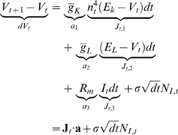
Compartmental models are spatially discrete approximations to the cable equation [13],[26],[27] and allow the temporal evolution of a compartment's voltage to be written as
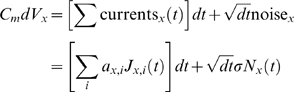 |
(1) |
where  is the voltage in compartment
  ,
,  is the specific membrane capacitance, and
  is current evolution noise (here assumed to be white and
Gaussian). Note the important factor
is current evolution noise (here assumed to be white and
Gaussian). Note the important factor  which ensures that the noise variance grows linearly with
time
which ensures that the noise variance grows linearly with
time  . The currents
  we will consider here are of three types:
- Axial currents along dendrites
(2) - Transmembrane currents from active (voltage-dependent), passive, or other (e.g. Ca2+ -dependent) membrane conductances

(3) - Experimentally injected currents
where
(4)  indicates one particular current type
(“channel”),
indicates one particular current type
(“channel”),  its reversal potential and
  its maximal conductance in compartment
  ,
,  is the membrane resistivity and
  is the current experimentally injected into that
compartment. The variable
is the current experimentally injected into that
compartment. The variable  represents the time-varying open fraction of the
conductance, and is typically given by complex, highly nonlinear
functions of time and voltage. For example, for the Hodgkin and
Huxley (HH) K+ -channel, the kinetics are given
by
represents the time-varying open fraction of the
conductance, and is typically given by complex, highly nonlinear
functions of time and voltage. For example, for the Hodgkin and
Huxley (HH) K+ -channel, the kinetics are given
by  , with
and
(5)  themselves nonlinear functions of the voltage
[28] and we again have an additive
noise term. In practice, the gate noise is either drawn from a
truncated Gaussian, or one can work with the transformed variable
themselves nonlinear functions of the voltage
[28] and we again have an additive
noise term. In practice, the gate noise is either drawn from a
truncated Gaussian, or one can work with the transformed variable  . Similar equations can be formulated for other
variables such as the intracellular free Ca2+
concentration [27].
. Similar equations can be formulated for other
variables such as the intracellular free Ca2+
concentration [27].
Noiseless observations
A detailed discussion of the case when the voltage is observed approximately
noiselessly (such as with a patch-clamp electrode) is presented in [23]
(see also [18],[21],[22]).
We here give a short review over the material on which the present work will
build. Let us henceforth assume that all the kinetics (such as  ) of all conductances are known. Once the voltage is known,
the kinetic equations can be evaluated to yield the open fraction
) of all conductances are known. Once the voltage is known,
the kinetic equations can be evaluated to yield the open fraction  of each conductance
  of interest. We further assume knowledge of the reversal
potentials
of interest. We further assume knowledge of the reversal
potentials  , although this can be relaxed, and of the membrane
specific capacitance
, although this can be relaxed, and of the membrane
specific capacitance  (which is henceforth neglected for notational clarity and
fixed at 1 nF/cm2; see [29] for a discussion
of this assumption).
(which is henceforth neglected for notational clarity and
fixed at 1 nF/cm2; see [29] for a discussion
of this assumption).
Knowledge of channel kinetics and voltage in each of the cell's
compartments allows inference of the linear parameters  and of the noise terms by constrained linear regression
[23]. As an example, consider a single-compartment
cell containing one active (Hodgkin-Huxley K+) and one
leak conductance and assume the voltage
and of the noise terms by constrained linear regression
[23]. As an example, consider a single-compartment
cell containing one active (Hodgkin-Huxley K+) and one
leak conductance and assume the voltage  has been recorded at sampling intervals
  for a time period of
  . Let
. Let  be the number of data points and
  index them successively
  :
:
 |
(6) |
where we see that only  ,
,  and
and  are now unknown; that they mediate the linear relationship
between
are now unknown; that they mediate the linear relationship
between  and
and  ; and that these parameters can be concatenated into a
vector
; and that these parameters can be concatenated into a
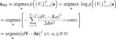
vector  as illustrated in equation 6. The maximum likelihood (ML)
estimate of
as illustrated in equation 6. The maximum likelihood (ML)
estimate of  (in vectorized form) and of
  are given by
 |
(7) |
| (8) |
where  . Note that the last equality in equation 7 expresses the
solution of the model fitting problem as a quadratic minimization with
linear constraints on the parameters and is straightforwardly performed with
standard packages such as quadprog.m in Matlab. The quadratic log-likelihood
in equation 7 and therefore the linear form of the regression depends on the
assumption that the evolution noise
. Note that the last equality in equation 7 expresses the
solution of the model fitting problem as a quadratic minimization with
linear constraints on the parameters and is straightforwardly performed with
standard packages such as quadprog.m in Matlab. The quadratic log-likelihood
in equation 7 and therefore the linear form of the regression depends on the
assumption that the evolution noise  of the observed variable in equation 6 is Gaussian white
noise. Parameters that can be simultaneously inferred in this manner from
the true voltage trace are
of the observed variable in equation 6 is Gaussian white
noise. Parameters that can be simultaneously inferred in this manner from
the true voltage trace are  ,
,  ,
,  , time-varying synaptic input strengths and the evolution
noise variances [23].
, time-varying synaptic input strengths and the evolution
noise variances [23].
In the following, we will write all the dynamical equations as simultaneous equations
| (9) |
where  is the evolution noise variance of the
  dynamic variable,
  if
if  and
and  denotes a vector of independent, identically distributed
(iid) random variables. These are Gaussian for unconstrained variables such
as the voltage, and drawn from truncated Gaussians for constrained variables
such as the gates. For the voltage we have
denotes a vector of independent, identically distributed
(iid) random variables. These are Gaussian for unconstrained variables such
as the voltage, and drawn from truncated Gaussians for constrained variables
such as the gates. For the voltage we have  and we remind ourselves that
  is a function of
  (equation 6).
Observation noise
Most recording techniques yield estimates of the underlying variable of
interest that are much more noisy than the essentially noise-free estimates
patch-clamping can provide. Imaging techniques, for example, do not provide
access to the true voltage which is necessary for the inference in equation
7. Figure 1 describes
the hidden dynamical system setting that applies to this situation.
Crucially, measurements  are instantaneously related to the underlying voltage
  by a probabilistic relationship (the turquoise arrows in
Figure 1) which is
dependent on the recording configuration. Together, the model of the
observations, combined with the (Markovian) model of the dynamics given by
the compartmental model define the following hidden dynamical system:
by a probabilistic relationship (the turquoise arrows in
Figure 1) which is
dependent on the recording configuration. Together, the model of the
observations, combined with the (Markovian) model of the dynamics given by
the compartmental model define the following hidden dynamical system:
| (10) |
| (11) |
where  denotes a Gaussian or truncated Gaussian distribution over
  with mean
  and variance
  and
and  denotes the linear measurement process (in the following
simply a linear projection such that
denotes the linear measurement process (in the following
simply a linear projection such that  or
or  ). We assume Gaussian noise both for the observations and
the voltage; and truncated Gaussian noise for the gates. The Gaussian
assumption on the evolution noise for the observed variable allows us to use
a simple regression (equation 7) in the inference of the channel densities.
Note that although the noise processes are i.i.d., the fact that noise is
injected into all gates means that the effective noise in the observations
can show strong serial correlations.
). We assume Gaussian noise both for the observations and
the voltage; and truncated Gaussian noise for the gates. The Gaussian
assumption on the evolution noise for the observed variable allows us to use
a simple regression (equation 7) in the inference of the channel densities.
Note that although the noise processes are i.i.d., the fact that noise is
injected into all gates means that the effective noise in the observations
can show strong serial correlations.
Figure 1. Hidden dynamical system.

The dynamical system comprises the hidden variables  and evolves as a Markov chain according to the
compartmental model and kinetic equations. The dynamical system is
hidden, because only noisy measurements of the true voltage are
observed. To perform inference, one has to take the observation
process
and evolves as a Markov chain according to the
compartmental model and kinetic equations. The dynamical system is
hidden, because only noisy measurements of the true voltage are
observed. To perform inference, one has to take the observation
process  into account. Inference is now possible because
the total likelihood of both observed and unobserved quantities
given the parameters can be expressed in terms of these two
probabilistic relations.
into account. Inference is now possible because
the total likelihood of both observed and unobserved quantities
given the parameters can be expressed in terms of these two
probabilistic relations.
Importantly, we do not assume that  bas the same dimensionality as
  ; in a typical cellular setting, there are several
unobserved variables per compartment, only one or a few of them being
measured. For Figure 2,
which illustrates the particle filter for a single-compartment model with
leak, Na+ and K+ Hodgkin-Huxley
conductances, only
; in a typical cellular setting, there are several
unobserved variables per compartment, only one or a few of them being
measured. For Figure 2,
which illustrates the particle filter for a single-compartment model with
leak, Na+ and K+ Hodgkin-Huxley
conductances, only  is measured, although the hidden variable
  is 4-dimensional and includes the three gates for the
Na+ and K+ channels in the
classical Hodgkin-Huxley model. It is, however, possible to have
is 4-dimensional and includes the three gates for the
Na+ and K+ channels in the
classical Hodgkin-Huxley model. It is, however, possible to have  of dimensionality equal to (or even greater than)
  . For example, [5] simultaneously
image voltage- and [Ca2+]-sensitive
dyes.
. For example, [5] simultaneously
image voltage- and [Ca2+]-sensitive
dyes.
Figure 2. Model-based smoothing.

A: Data; generated by adding Gaussian noise
(σO = 30
mV) to the voltage trace and subsampling every seven timesteps
(Δ = 0.02 ms and Δs = 0.14 ms). The voltage
trace was generated by running the equation 1 for the single
compartment with the correct parameters once and adding noise of
variance  . B: Voltage paths corresponding to the
  particles which were run with the correct, known
parameters. C: Effective particle number
particles which were run with the correct, known
parameters. C: Effective particle number  . As soon as enough particles have
‘drifted’ away from the data (
. As soon as enough particles have
‘drifted’ away from the data ( reaches the threshold
  ), a resampling step eliminates the stray particles
(they are reset to a particle with larger weight) all weights are
reset to
), a resampling step eliminates the stray particles
(they are reset to a particle with larger weight) all weights are
reset to  and the effective number returns to
  . D: expected voltage trace
 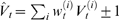 st. dev. in shaded colours. The mean reproduces
the underlying voltage trace with high accuracy. E: Conditional
expectations for the gates of the particles (mean ±1 st.
dev.); blue: HH
st. dev. in shaded colours. The mean reproduces
the underlying voltage trace with high accuracy. E: Conditional
expectations for the gates of the particles (mean ±1 st.
dev.); blue: HH  ; green: HH
  ; red: HH
  . Thus, using model-based smoothing, a highly
accurate estimate of the underlying voltage and the gates can be
recovered from very noisy, undersampled data.
. Thus, using model-based smoothing, a highly
accurate estimate of the underlying voltage and the gates can be
recovered from very noisy, undersampled data.
Expectation-Maximisation
Expectation-Maximisation (EM) is one standard machine-learning technique that allows estimation of parameters in precisely the circumstances just outlined, i.e. where inference depends on unobserved variables and certain expectations can be evaluated. The EM algorithm achieves a local maximisation of the data likelihood by iterating over two steps. For the case where voltage is recorded, it consists of:
Expectation step (E-Step): The parameters are fixed at their current estimate
 ; based on this (initally inaccurate) parameter
setting, the conditional distribution of the hidden variables
; based on this (initally inaccurate) parameter
setting, the conditional distribution of the hidden variables  (where
  are all the observations) is inferred. This
effectively amounts to model-based smoothing of the noisy data and will
be discussed in the first part of the paper.
are all the observations) is inferred. This
effectively amounts to model-based smoothing of the noisy data and will
be discussed in the first part of the paper.Maximisation step (M-Step): Based on the model-based estimate of the hidden variables
 , a new estimate of the parameters
  is inferred, such that it maximises the expected joint
log likelihood of the observations and the inferred distribution over
the unobserved variables. This procedure is a generalisation of
parameter inference in the case mentioned in equation 7, where the
voltage was observed noiselessly.
is inferred, such that it maximises the expected joint
log likelihood of the observations and the inferred distribution over
the unobserved variables. This procedure is a generalisation of
parameter inference in the case mentioned in equation 7, where the
voltage was observed noiselessly.
The EM algorithm can be shown to increase the likelihood of the parameters at each iteration [24],[25],[30],[31], and will typically converge to a local maximum. Although in combination with the Monte-Carlo estimation these guarantees no longer hold, in practice, we have never encountered nonglobal optima.
Methods
Model-based smoothing
We first assume that the true parameters  are known, and in the E-step infer the conditional marginal
distributions
are known, and in the E-step infer the conditional marginal
distributions  for all times
  . The conditional mean
  is a model-based, smoothed estimate of the true underlying
signal
is a model-based, smoothed estimate of the true underlying
signal  at each point in time
  which is optimal under mean squared error. The E-step is
implemented using standard sequential Monte Carlo techniques [7].
Here we present the detailed equations as applied to noisy recordings of
cellular dynamic variables such as the transmembrane voltage or intracellular
calcium concentration.
which is optimal under mean squared error. The E-step is
implemented using standard sequential Monte Carlo techniques [7].
Here we present the detailed equations as applied to noisy recordings of
cellular dynamic variables such as the transmembrane voltage or intracellular
calcium concentration.
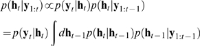
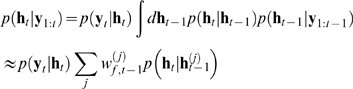
The smoothed distribution  is computed via a backward recursion which relies on the
filtering distribution
is computed via a backward recursion which relies on the
filtering distribution  , which in turn is inferred by writing the following recursion
(suppressing the dependence on
, which in turn is inferred by writing the following recursion
(suppressing the dependence on  for clarity):
 |
(12) |
This recursion relies on the fact that the hidden variables are Markovian
| (13) |
Based on this, the smoothed distribution, which gives estimates
of the hidden variables that incorporate all, not just the past, observations,
can then be inferred by starting with  and iterating backwards:
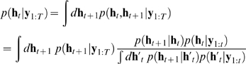 |
(14) |
where all quantities inside the integral are now known.
Sequential Monte Carlo
The filtering and smoothing equations demand integrals over the hidden variables.
In the present case, these integrals are not analytically tractable, because of
the complex nonlinearities in the kinetics  . They can, however, be approximated using Sequential Monte
Carlo methods. Such methods (also known as “particle
filters”) are a special version of importance sampling, in which
distributions and expectations are represented by weighted samples
. They can, however, be approximated using Sequential Monte
Carlo methods. Such methods (also known as “particle
filters”) are a special version of importance sampling, in which
distributions and expectations are represented by weighted samples 
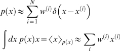 |
with  . If samples are drawn from the distribution
  directly, the weights
  . In the present case, this would mean drawing samples from the
distributions
. In the present case, this would mean drawing samples from the
distributions  and
and  , which is not possible because they themselves depend on
integrals at adjacent timesteps which are hard to evaluate exactly. Instead,
importance sampling allows sampling from a different
“proposal” distribution
, which is not possible because they themselves depend on
integrals at adjacent timesteps which are hard to evaluate exactly. Instead,
importance sampling allows sampling from a different
“proposal” distribution  and compensating by setting
  . Here, we first seek samples and forward filtering weights
  such that
| (15) |
and based on these will then derive backwards, smoothing weights such that
| (16) |
Substituting the desideratum in equation 15 for time  into equation 12
 |
(17) |
As a proposal distribution for our setting we use the one-step predictive probability distribution (derived from the Markov property in equation 13):
| (18) |
where  is termed the
  “particle”. The samples are made to
reflect the conditional distribution by adjusting the weights, for which the
probabilities
“particle”. The samples are made to
reflect the conditional distribution by adjusting the weights, for which the
probabilities  need to be computed. These are given by
which involves a sum over  that is quadratic in
  . We approximate this by
| (19) |
which neglects the probability that the particle  at time
  could in fact have arisen from particle
  at time
  . The weights for each of the particles are then given by a
simple update equation:
. The weights for each of the particles are then given by a
simple update equation:
| (20) |
 |
(21) |
One well-known consequence of the approximation in equations 19–21 is
that over time, the variance of the weights becomes large; this means that most
particles have negligible weight, and only one particle is used to represent a
whole distribution. Classically, this problem is prevented by resampling, and we
here use stratified resampling [8]. This procedure, illustrated in Figure 2, results in
eliminating particles that assign little, and duplicating particles that assign
large likelihood to the data whenever the effective number of particles  drops below some threshold, here
  .
.
It should be pointed out that it is also possible to interpolate between
observations, or to do learning (see below) from subsampled traces. For example,
assume we have a recording frequency of  but wish to infer the underlying signal at a higher frequency
  , with
  . At time points without observation the likelihood term in
equation 21 is uninformative (flat) and we therefore set
. At time points without observation the likelihood term in
equation 21 is uninformative (flat) and we therefore set
| (22) |
keeping equation 21 for the remainder of times. In this paper, we
will run compartmental models (equation 1) at sampling intervals  , and recover signals to that same temporal precision from data
subsampled at intervals
, and recover signals to that same temporal precision from data
subsampled at intervals  . See e.g. [32] for further details on incorporating
intermittently-sampled observations into the alternative predictive distribution
. See e.g. [32] for further details on incorporating
intermittently-sampled observations into the alternative predictive distribution  .
.
We have so far derived the filtering weights such that particles are
representative of the distribution conditioned on the past data  . It often is more appropriate to condition on the entire set
of measurements, i.e. represent the distribution
. It often is more appropriate to condition on the entire set
of measurements, i.e. represent the distribution  . We will see that this is also necessary for the parameter
inference in the M-step. Substituting equations 15 and 16 into equation 14, we
arrive at the updates for the smoothing weights
. We will see that this is also necessary for the parameter
inference in the M-step. Substituting equations 15 and 16 into equation 14, we
arrive at the updates for the smoothing weights
 |
where the weights  now represent the joint distribution of the hidden variables
at adjacent timesteps:
now represent the joint distribution of the hidden variables
at adjacent timesteps:
Parameter inference
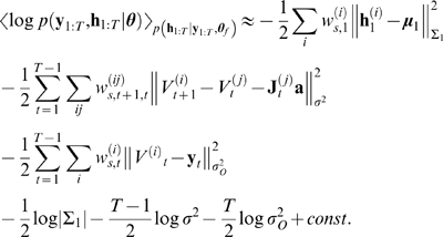
The maximum likelihood estimate of the parameters can be inferred via a maximisation of an expectation over the hidden variables:
where  . This is achieved by iterating over the two steps of the EM
algorithm. In the M-step of the
. This is achieved by iterating over the two steps of the EM
algorithm. In the M-step of the  iteration, the likelihood of the entire set of measurements
  with respect to the parameters
  is maximised by maximising the expected total log likelihood
[25]
is maximised by maximising the expected total log likelihood
[25]
which is achieved by setting the gradients with respect to  to zero (see [31],[33] for
alternative approaches). For the main linear parameters we seek to infer in the
compartmental model (
to zero (see [31],[33] for
alternative approaches). For the main linear parameters we seek to infer in the
compartmental model ( ), these equations are solved by performing a constrained
linear regression, akin to that in equation 7. We write the total likelihood in
terms of the dynamic and the observation models (equations 10 and 11):
), these equations are solved by performing a constrained
linear regression, akin to that in equation 7. We write the total likelihood in
terms of the dynamic and the observation models (equations 10 and 11):
Let us assume that we have noisy measurements of the voltage.
Because the parametrisation of the evolution of the voltage is linear, but that
of the other hidden variables is not, we separate the two as  where
where  are the gates of the conductances affecting the voltage (a
similar formulation can be written for
[Ca2+] observations). Approximating the
expectations by the weighted sums of the particles defined in the previous
section, we arrive at
are the gates of the conductances affecting the voltage (a
similar formulation can be written for
[Ca2+] observations). Approximating the
expectations by the weighted sums of the particles defined in the previous
section, we arrive at
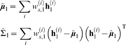
 |
(23) |
where 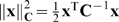 ,
,  and
and  parametrise the distribution
  over the initial hidden variables at time
  , and
, and  is the
  row of the matrix
  derived from particle
  . Note that because we are not inferring the kinetics of the
channels, the evolution term for the gates (a sum over terms of the form
. Note that because we are not inferring the kinetics of the
channels, the evolution term for the gates (a sum over terms of the form 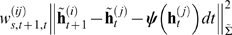 ) is a constant and can be neglected. Now setting the gradients
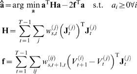
of equation 23 with respect to the parameters to zero, we find that the linear
parameters can be written, as in equation 7, as a straightforward quadratic
minimisation with linear constraints
) is a constant and can be neglected. Now setting the gradients
of equation 23 with respect to the parameters to zero, we find that the linear
parameters can be written, as in equation 7, as a straightforward quadratic
minimisation with linear constraints
 |
(24) |
where we see that the Hessian  and the linear term
  of the problem are given by an expectation involving the
particles. Importantly, this is still a quadratic optimisation problem with
linear constraints, and which is efficiently solved by standard packages.
Similarly, the initialisation parameters for the unobserved hidden variables are
given by
of the problem are given by an expectation involving the
particles. Importantly, this is still a quadratic optimisation problem with
linear constraints, and which is efficiently solved by standard packages.
Similarly, the initialisation parameters for the unobserved hidden variables are
given by
 |
which are just the conditional mean and variance of the particles
at time  ; and the evolution and observation noise terms finally by
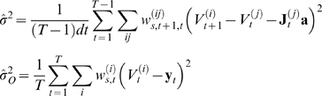 |
Thus, the procedure iterates over running the particle smoother in section Sequential Monte Carlo and then inferring the optimal parameters from the smoothed estimates of the unobserved variables.
Results
Model-based smoothing
We first present results on model-based smoothing. Here, we assume that we have a
correct description of the parameters of the cell under
scrutiny, and use this description to infer the true underlying signal from
noisy measurements. These results may be considered as one possible application
of a detailed model. Figure
2A shows the data, which was generated from a known, single-compartment
cell with Hodgkin-Huxley-like conductances by adding Gaussian noise. The
variance of the noise was chosen to replicate typical signal-to-noise ratios
from voltage-dye experiments [2]. Figure 2B shows the  particles used here, and Figure 2C the number of particles with
non-negligible weights (the “effective” number
particles used here, and Figure 2C the number of particles with
non-negligible weights (the “effective” number  of particles). We see that when
  hits a threshold of
  , resampling results in large jumps in some particles. At
around 3 ms, we see that some particles, which produced a spike at a time when
there is little evidence for it in the data, are re-set to a value that is in
better accord with the data. Figure
2D shows the close match between the true underlying signal and the
inferred mean
, resampling results in large jumps in some particles. At
around 3 ms, we see that some particles, which produced a spike at a time when
there is little evidence for it in the data, are re-set to a value that is in
better accord with the data. Figure
2D shows the close match between the true underlying signal and the
inferred mean  , while Figure
2E shows that even the unobserved channel open fractions are inferred
very accurately. The match for both the voltage and the open channel fractions
improves with the number of particles. Code for the implementation of this
smoothing step is available online at http://www.gatsby.ucl.ac.uk/˜qhuys/code.html.
, while Figure
2E shows that even the unobserved channel open fractions are inferred
very accurately. The match for both the voltage and the open channel fractions
improves with the number of particles. Code for the implementation of this
smoothing step is available online at http://www.gatsby.ucl.ac.uk/˜qhuys/code.html.
For imaging data, the laser often has to be moved between recording locations, leading to intermittent sampling at any one location (see [34]–[36]). Figure 3 illustrates the performance of the model-based smoother both for varying noise levels and for temporal subsampling. We see that even for very noisy and highly subsampled data, the spikes can be recovered very well.
Figure 3. Performance of the model-based smoother with varying observation
noise  and temporal subsampling
  .
.

True underlying voltage trace in dashed black lines, the  particles in gray and the data in black circles.
Accurate inference of underlying voltage signals, and thus of spike
times, is possible with accurate descriptions of the cell, over a wide
range of noise levels and even at low sampling frequencies.
particles in gray and the data in black circles.
Accurate inference of underlying voltage signals, and thus of spike
times, is possible with accurate descriptions of the cell, over a wide
range of noise levels and even at low sampling frequencies.
Figure 4 shows a different
aspect of the same issue, whereby the laser moves linearly across an extended
linear dendrite. Here, samples are taken every  timesteps, but samples from each individual compartment are
only obtained each
timesteps, but samples from each individual compartment are
only obtained each  . The true voltage across the entire passive dendrite is shown
in Figure 4A, and the sparse
data points distributed over the dendrite are shown in panel B. The inferred
mean in panel C matches the true voltage very well. For this
passive, linear example, the equations for the hidden dynamical
system are exactly those of a Kalman smoother model [37]; thus the standard
Kalman smoother performs the correct spatial and temporal smoothing once the
parameters are known, with no need for the more general (but more
computationally costly) particle smoother introduced above. More precisely, in
this case the integrals in equations 12 and 14 can be evaluated analytically,
and no sampling is necessary. The supplemental video S1
shows the results of a similar linear (passive-membrane) simulation, performed
on a branched simulated dendrite (instead of the linear dendritic segment
illustrated in Figure 4).
. The true voltage across the entire passive dendrite is shown
in Figure 4A, and the sparse
data points distributed over the dendrite are shown in panel B. The inferred
mean in panel C matches the true voltage very well. For this
passive, linear example, the equations for the hidden dynamical
system are exactly those of a Kalman smoother model [37]; thus the standard
Kalman smoother performs the correct spatial and temporal smoothing once the
parameters are known, with no need for the more general (but more
computationally costly) particle smoother introduced above. More precisely, in
this case the integrals in equations 12 and 14 can be evaluated analytically,
and no sampling is necessary. The supplemental video S1
shows the results of a similar linear (passive-membrane) simulation, performed
on a branched simulated dendrite (instead of the linear dendritic segment
illustrated in Figure 4).
Figure 4. Inferring spatiotemporal voltage distribution from scanning, intermittent samples.

A: True underlying voltage signal as a function of time for all 15 compartments. This was generated by injecting white noise current into a passive cell containing 50 linearly arranged compartments. B: Samples obtained by scanning repeatedly along the dendrite. The samples are seen as diagonal lines extending downwards, ie each compartment was sampled in sequence, overall 10 times and 25 ms apart. Note that the samples were noisy (σO = 3.16 mV). C: Conditional expected voltage time course for all compartments reconstructed by Kalman smoothing. The colorbar indicates the voltage for all three panels. Note that even though there is only sparse data over time and space, a smooth version of the full spatiotemporal pattern is recovered. D: Variance of estimated voltage. It is smallest at the observation times and rapidly reaches a steady state between observations. Due to the smoothing, which takes future data into account, the variance diminishes ahead of observations.
We emphasize that the strong performance of the particle smoother and the Kalman smoother here should not be surprising, since the data were generated from a known model and in these cases these methods perform smoothing in a statistically optimal manner. Rather, these results should illustrate the power of using an exact, correct description of the cell and its dynamics.
EM – inferring cellular parameters
We have so far shown model-based filtering assuming that a full model of the cell
under scrutiny is available. Here, we instead infer some of the main parameters
from the data; specifically the linear parameters  , the observation noise
  and the evolution noise
  . We continue to assume, however, that the kinetics of all
channels that may be present in the cell are known exactly (see [23] for a
discussion of this assumption).
. We continue to assume, however, that the kinetics of all
channels that may be present in the cell are known exactly (see [23] for a
discussion of this assumption).
Figure 5 illustrates the
inference for a passive multicompartmental model, similar to that in Figure 4, but driven by a
square current injection into the second compartment. Figure 5B shows statistics of the inference
of the leak conductance maximal density  , the intercompartmental conductance
  , the input resistance
  and the observation noise
  across 50 different randomly generated noisy voltage traces.
All the parameters are reliably recovered from 2 seconds of data at a 1 ms
sampling frequency.
across 50 different randomly generated noisy voltage traces.
All the parameters are reliably recovered from 2 seconds of data at a 1 ms
sampling frequency.
Figure 5. Inferring biophysical parameters from noisy measurements in a passive cell.

A: True voltage (black) and noisy data (grey dots) from the 5
compartments of the cell with noise level
σO = 10
mV. B–E: Parameter inference with EM. Each panel shows the
average inference time course±one st. dev. of one of the
cellular parameters. B: Leak conductance; C: intercompartmental
conductance; D: input resistivity; E: Observation noise variance. The
grey dotted line shows the true values. The coloured lines show the
inference for varying levels of noise  . Blue:
σO = 1
mV, Green:
σO = 5
mV, Red:
σO = 10
mV, Cyan:
σO = 20
mV, Magenta:
σO = 50
mV. Throughout Δs = 1
ms = 10Δ. Note that accurate
estimation of the leak, input resistance and noise levels is even
possible when the noise is five times as large as that shown in panel A.
Inference of the intercompartmental conductance suffers most from the
added noise because the small intercompartmental currents have to be
distinguished from the apparent currents arising from noise fluctuations
in the observations from neighbouring compartments. Throughout, the
underlying voltage was estimated highly accurately (data not shown),
which is also reflected in the accurate estimates of
. Blue:
σO = 1
mV, Green:
σO = 5
mV, Red:
σO = 10
mV, Cyan:
σO = 20
mV, Magenta:
σO = 50
mV. Throughout Δs = 1
ms = 10Δ. Note that accurate
estimation of the leak, input resistance and noise levels is even
possible when the noise is five times as large as that shown in panel A.
Inference of the intercompartmental conductance suffers most from the
added noise because the small intercompartmental currents have to be
distinguished from the apparent currents arising from noise fluctuations
in the observations from neighbouring compartments. Throughout, the
underlying voltage was estimated highly accurately (data not shown),
which is also reflected in the accurate estimates of  .
.
We now proceed to infer channel densities and observation noise from active
compartments with either four or eight channels. Figure 6 shows an example trace and inference
for the four channel case (using Hodgkin-Huxley like channel kinetics). Again,
we stimulated with square current pulses. Only 10 ms of data were recorded, but
at a very high temporal resolution Δs = Δ = 0.02
ms. We see that both the underlying voltage trace and the channel and input
resistance are recovered with high accuracy. Figure 7 presents batch data over 50 runs for
varying levels of observation noise  . The observation noise here has two effects: first, it slows
down the inference (as every data point is less informative), but secondly the
variance across runs increases with increasing noise (although the mean is still
accurate). For illustration purposes, we started the maximal
K+ conductance at its correct value. As can be seen,
however, the inference initially moves
. The observation noise here has two effects: first, it slows
down the inference (as every data point is less informative), but secondly the
variance across runs increases with increasing noise (although the mean is still
accurate). For illustration purposes, we started the maximal
K+ conductance at its correct value. As can be seen,
however, the inference initially moves  away from the optimum, to compensate for the other conductance
misestimations. (This nonmonotonic behavior in
away from the optimum, to compensate for the other conductance
misestimations. (This nonmonotonic behavior in  is a result of the fact that the EM algorithm is searching for
an optimal setting of all of the cell's conductance parameters, not
just a single parameter; we will return to this issue below.)
is a result of the fact that the EM algorithm is searching for
an optimal setting of all of the cell's conductance parameters, not
just a single parameter; we will return to this issue below.)
Figure 6. Example inference for single compartment with active conductances.

A: Noisy data, σO = 10 mV; B: True underlying voltage (black dashed line) resulting from current pulse injection shown in E. The gray trace shows the mean inferred voltage after inferring the paramter values in C. C: Initial (blue +) and inferred parameter values (red ×) in percent relative to true values (gray bars ḡ Na = 120 mS/cm2, ḡ K = 20 mS/cm2, ḡ Leak = 3 mS/cm2, Rm = 1 mS/cm2). At the initial values the cell was non-spiking. D: Magnified view showing data, inferred and true voltage traces for the first spike. Thus, despite the very high noise levels and an initially inaccurate, non-spiking model of the cell, knowledge of the channel kinetics allows accurate inference of the channel densities and very precise reconstruction of the underlying voltage trace.
Figure 7. Time course of parameter estimation with HH channels.

The four panels show, respectively, the inference for the conductance
parameters A:  B:
B:  C:
C:  and D:
  . The thick coloured lines indicate the mean over 50
data samples and the shaded areas 1 st. dev. The colours indicate
varying noise levels
. The thick coloured lines indicate the mean over 50
data samples and the shaded areas 1 st. dev. The colours indicate
varying noise levels  . Blue:
σO = 1
mV, Green:
σO = 5
mV, Red:
σO = 10
mV, Cyan:
σO = 20
mV. The true parameters are indicated by the horizontal gray dashed
lines. Throughout Δs = Δ = 0.02
ms. The main effect of increasing observation noise is to slow down the
inference. In addition, larger observation noise also adds variance to
the parameter estimates. Throughout, only 10 ms of data were used.
. Blue:
σO = 1
mV, Green:
σO = 5
mV, Red:
σO = 10
mV, Cyan:
σO = 20
mV. The true parameters are indicated by the horizontal gray dashed
lines. Throughout Δs = Δ = 0.02
ms. The main effect of increasing observation noise is to slow down the
inference. In addition, larger observation noise also adds variance to
the parameter estimates. Throughout, only 10 ms of data were used.
Parametric inference here has so far employed densely sampled traces (see Figure 6A). The algorithm however applies equally to subsampled traces (see equation 22). Figure 8 shows the effect of subsampling. We see that subsampling, just as noise, slows down the inference, until the active conductances are no longer inferred accurately (the yellow trace for Δs = 0.5 ms). In this case, the total recording length of 10 ms meant that inference had to be done based on one single spike. For longer recordings, information about multiple spikes can of course be combined, partially alleviating this problem; however, we have found that in highly active membranes, sampling frequencies below about 1 KHz led to inaccurate estimates of sodium channel densities (since at slower sampling rates we will typically miss significant portions of the upswing of the action potential, leading the EM algorithm to underestimate the sodium channel density). Note that we kept the length of the recording in Figure 8 constant, and thus subsampling reduced the total number of measurements.
Figure 8. Subsampling slows down parametric inference.

Inference of the same parameters as in previous Figure (A:  , B:
, B:  , C:
, C:  , D:
, D:  ), but the different colours now indicate increasing
subsampling. Particles evolved at timesteps of
Δ = 0.04 ms. The coloured
traces inference with show sampling timesteps of Δs = {0.01,0.02,0.05,0.1,0.5} ms
respectively. All particles were run with a
Δ = 0.01 ms timestep, and the
total recording was always 10 ms long, meaning that progressive
subsampling decreased the total number of data points. Thus, it can be
seen that parameter inference is quite relatively to undersampling. At
very large subsampling times, 10 ms of data supplied too few
observations during a spike to justify inference of high levels of
Na+ and K+ conductances, but
the input resistance and the leak were still reliably and accurately
inferred.
), but the different colours now indicate increasing
subsampling. Particles evolved at timesteps of
Δ = 0.04 ms. The coloured
traces inference with show sampling timesteps of Δs = {0.01,0.02,0.05,0.1,0.5} ms
respectively. All particles were run with a
Δ = 0.01 ms timestep, and the
total recording was always 10 ms long, meaning that progressive
subsampling decreased the total number of data points. Thus, it can be
seen that parameter inference is quite relatively to undersampling. At
very large subsampling times, 10 ms of data supplied too few
observations during a spike to justify inference of high levels of
Na+ and K+ conductances, but
the input resistance and the leak were still reliably and accurately
inferred.
As with any importance sampling method, particle filtering is known to suffer in
higher dimensions [38]. To investigate the dependence of the
particle smoother's accuracy on the dimensionality of the state space,
we applied the method to a compartment with a larger number of channels: fast ( ) and persistent Na+ (
 ) channels in addition to leak (L) and delayed rectivier (
 ), A-type (
 ), K2-type (K2) and M-type (
 ) K+ channels (channel kinetics from
ModelDB [39], from [9],[40]). Figure 9 shows the evolution
of the channel intensities during inference. Estimates of most channel densities
are correct up to a factor of approximately 2. Unlike in the previous, smaller
example, as either observation noise or subsampling increase, significant biases
in the estimation of channel densities appear. For instance, the density of the
fast sodium channel observed with noise of standard deviation 20 mV is only
about half the true value.
) K+ channels (channel kinetics from
ModelDB [39], from [9],[40]). Figure 9 shows the evolution
of the channel intensities during inference. Estimates of most channel densities
are correct up to a factor of approximately 2. Unlike in the previous, smaller
example, as either observation noise or subsampling increase, significant biases
in the estimation of channel densities appear. For instance, the density of the
fast sodium channel observed with noise of standard deviation 20 mV is only
about half the true value.
Figure 9. Time course of parameter estimation in a model with eight conductances.

Evolution of estimates of channel densities for compartment with eight
channels. Colours show inference with changes in the observation noise  and the subsampling
  . True levels are indicated by dotted gray lines. A: Δs = .02 ms,
σO = {1,2,5,10,20}
mV respectively for blue, green, red, cyan and purple lines B:
σO = 5
mV, Δs = {.02,.04,.1,.2,.4} ms again
for blue, green, red, cyan and purple lines respectively. Thick lines
show median, thin lines show 10 and 90% quantiles of
distribution across 50 runs.
. True levels are indicated by dotted gray lines. A: Δs = .02 ms,
σO = {1,2,5,10,20}
mV respectively for blue, green, red, cyan and purple lines B:
σO = 5
mV, Δs = {.02,.04,.1,.2,.4} ms again
for blue, green, red, cyan and purple lines respectively. Thick lines
show median, thin lines show 10 and 90% quantiles of
distribution across 50 runs.
It is worth noting that this bias problem is not observed in the passive linear case, where the analytic Kalman smoother suffices to perform the inference: we can infer the linear dynamical parameters of neurons with many compartments, as long as we sample information from each compartment [23]. Instead, the difficulty here is due to multicollinearity of the regression performed in the M-step of the EM algorithm and to the fact that the particle smoother leads to biased estimation of covariance parameters in high-dimensional cases [38]. We will discuss some possible remedies for these biases below.
Somewhat surprisingly, however, these observed estimation biases do not prove
catastrophic if we care about predicting or smoothing the subthreshold voltage.
Figure 10A compares the
response to a new, random, input current of a compartment with the true
parameters to that of a compartment with parameters as estimated during EM
inference, while Figure 10B
shows an example prediction with 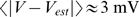 . Note the large plateau potentials after the spikes due to the
persistent sodium channel
. Note the large plateau potentials after the spikes due to the
persistent sodium channel  . We see that even the parameters as estimated under high noise
accurately come to predict the response to a new, previously unseen, input
current. The asymptote in Figure
10A is determined by the true evolution noise level (here
σ = 1 mV): the
more inherent noise, the less a response to a specific input is actually
predictable.
. We see that even the parameters as estimated under high noise
accurately come to predict the response to a new, previously unseen, input
current. The asymptote in Figure
10A is determined by the true evolution noise level (here
σ = 1 mV): the
more inherent noise, the less a response to a specific input is actually
predictable.
Figure 10. Predictive performance of inferred parameter settings on new input current.

A: Parameter estimates as shown in Figure 9A were used to predict response to a new input stimulus. The plot shows the absolute error averaged over the entire trace (3000 timesteps, Δt = .02 ms), for 40 runs. Thick lines show the median, shaded areas 10 and 90% quantiles over the same 40 runs as in Figure 9. Blue: σO = 1 mV, Green: σO = 2 mV, Red: σO = 5 mV, Cyan: σO = 10 mV, Magenta: σO = 20 mV. Note logarithmic y axis. B: Example prediction trace. The dashed black line shows the response of the cell with the true parameters, the red line that with the inferred parameters. The observation noise was σO = 20 mV, while the average error for this trace 〈|V−Vest|〉 = 2.96 mV.
Some further insight into the problem can be gained by looking at the structure
of the Hessian of the total likelihood  around the true parameters. We estimate
  by running the particle smoother with a large number of
particles once at the true parameter value; more generally, one could perform a
similar analysis about the inferred parameter setting to obtain a parametric
bootstrap estimate of the posterior uncertainty. Figure 11 shows that, around the true value,
changes in either the fast Na+ or the K2-type
K+ channel have the least effect; i.e., the curvature in
the loglikelihood is smallest in these directions, indicating that the observed
data does not adequately constrain our parameter estimates in these directions,
and prior information must be used to constrain these estimates instead. This
explains why these channels showed disproportionately large amounts of inference
variability, and why the prediction error did not suffer catastrophically from
their relatively inaccurate inference (Figure 10A). See [23] for further
discussion of this multicollinearity issue in large multichannel models.
by running the particle smoother with a large number of
particles once at the true parameter value; more generally, one could perform a
similar analysis about the inferred parameter setting to obtain a parametric
bootstrap estimate of the posterior uncertainty. Figure 11 shows that, around the true value,
changes in either the fast Na+ or the K2-type
K+ channel have the least effect; i.e., the curvature in
the loglikelihood is smallest in these directions, indicating that the observed
data does not adequately constrain our parameter estimates in these directions,
and prior information must be used to constrain these estimates instead. This
explains why these channels showed disproportionately large amounts of inference
variability, and why the prediction error did not suffer catastrophically from
their relatively inaccurate inference (Figure 10A). See [23] for further
discussion of this multicollinearity issue in large multichannel models.
Figure 11. Eigenstructure of Hessian  with varying observation noise.

Eigenvector 1 has the largest (>104), and eigenvector 8 respectively the smallest eigenvalue (∼0.5). Independently of the noise, the smalles eigenvectors involve those channels for which inference in Figure 9 appeared least reliable: the fast Na+ and the K2-type K+ channel.
Estimation of subthreshold nonlinearity by nonparametric EM
We saw in the last section that as the dimensionality of the state vector  grows, we may lose the ability to simultaneously estimate all
of the system parameters. How can we deal with this issue? One approach is to
take a step back: in many statistical settings we do not care primarily about
estimating the underlying model parameters accurately, but rather we just need a
model that predicts the data well. It is worth emphasizing that the methods we
have intrduced here can be quite useful in this setting as well. As an important
example, consider the problem of estimating the subthreshold voltage given noisy
observations. In many applications, we are more interested in a method which
will reliably extract the subthreshold voltage than in the parameters underlying
the method. For example, if a linear smoother (e.g., the Kalman smoother
discussed above) works well, it might be more efficient and stable to stick with
this simpler method, rather than attempting to estimate the parameters defining
the cell's full complement of active membrane channels (indeed,
depending on the signal-to-noise ratio and the collinearity structure of the
problem, the latter goal may not be tractable, even in cases where the voltage
may be reliably measured [23]).
grows, we may lose the ability to simultaneously estimate all
of the system parameters. How can we deal with this issue? One approach is to
take a step back: in many statistical settings we do not care primarily about
estimating the underlying model parameters accurately, but rather we just need a
model that predicts the data well. It is worth emphasizing that the methods we
have intrduced here can be quite useful in this setting as well. As an important
example, consider the problem of estimating the subthreshold voltage given noisy
observations. In many applications, we are more interested in a method which
will reliably extract the subthreshold voltage than in the parameters underlying
the method. For example, if a linear smoother (e.g., the Kalman smoother
discussed above) works well, it might be more efficient and stable to stick with
this simpler method, rather than attempting to estimate the parameters defining
the cell's full complement of active membrane channels (indeed,
depending on the signal-to-noise ratio and the collinearity structure of the
problem, the latter goal may not be tractable, even in cases where the voltage
may be reliably measured [23]).
Of course, in many cases linear smoothers are not appropriate. For example, the linear (Kalman) model typically leads to oversmoothing if the voltage dynamics are sufficiently nonlinear (data not shown), because action potentials take place on a much faster timescale than the passive membrane time constant. Thus it is worth looking for a method which can incorporate a flexible nonlinearity and whose parameters may not be directly interpretable biophysically but which nonetheless leads to good estimation of the signal of interest. We could just throw a lot of channels into the mix, but this increases the dimensionality of the state space, hurting the performance of the particle smoother and leading to multicollinearity problems in the M-step, as illustrated in the last subsection.
A more promising approach is to fit nonlinear dynamics directly, while keeping the dimensionality of the state space as small as possible. This has been a major theme in computational neuroscience, where the reduction of complicated multichannel models into low-dimensional models, useful for phase plane analysis, has led to great insights into qualitative neural dynamics [26],[41].
As a concrete example, we generated data from a strongly nonlinear (Fitzhugh-Nagumo) two-dimensional model, and then attempted to perform optimal smoothing, without prior knowledge of the underlying voltage nonlinearity. We initialized our analysis with a linear model, and then fit the nonlinearity nonparametrically via a straightforward nonparametric modification of the EM approach developed above.
In more detail, we generated data from the following model [41]:
| (25) |
| (26) |
where the nonlinear function  is cubic in this case, and
  and
and  denote independent white Gaussian noise processes. Then, given
noisy observations of the voltage
denote independent white Gaussian noise processes. Then, given
noisy observations of the voltage  (Figure
12, left middle panel), we used a nonparametric version of our EM
algorithm to estimate
(Figure
12, left middle panel), we used a nonparametric version of our EM
algorithm to estimate  . The E-step of the EM algorithm is unchanged in this context:
we compute
. The E-step of the EM algorithm is unchanged in this context:
we compute  and
and  , along with the other pairwise sufficient statistics, using
our standard particle forward-backward smoother, given our current estimate of
, along with the other pairwise sufficient statistics, using
our standard particle forward-backward smoother, given our current estimate of  . The M-step here is performed using a penalized spline method
[42]: we represent
. The M-step here is performed using a penalized spline method
[42]: we represent  as a linearly weighted combination of fixed basis functions
  :
:
and then determine the optimal weights  by maximum penalized likelihood:
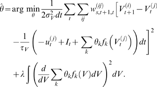 |
The first term here corresponds to the expected complete
loglikelihood (as in equation (23)), while the second term is a penalty which
serves to smooth the inferred function  (by penalizing non-smooth solutions, i.e., functions
  whose derivative has a large squared norm); the scalar
  serves to set the balance between the smoothness of
  and the fit to the data. Despite its apparent complexity, in
fact this expression is just a quadratic function of
and the fit to the data. Despite its apparent complexity, in
fact this expression is just a quadratic function of  (just like equation (24)), and the update
  may be obtained by solving a simple linear equation. If the
basis functions
may be obtained by solving a simple linear equation. If the
basis functions  have limited overlap, then the Hessian of this objective
function with respect to
have limited overlap, then the Hessian of this objective
function with respect to  is banded (with bandwidth equal to the degree of overlap in
the basis functions
is banded (with bandwidth equal to the degree of overlap in
the basis functions  ), and therefore this linear equation can be solved quickly
using sparse banded matrix solvers [42],[43].
We used 50 nonoverlapping simple step functions to represent
), and therefore this linear equation can be solved quickly
using sparse banded matrix solvers [42],[43].
We used 50 nonoverlapping simple step functions to represent  in Figures.
12–13,
and each M-step took negligible time (≪1 sec). The penalty term
in Figures.
12–13,
and each M-step took negligible time (≪1 sec). The penalty term  was fit crudely by eye here (we chose a
  that led to a reasonable fit to the data, without drastically
oversmoothing
that led to a reasonable fit to the data, without drastically
oversmoothing  ); this could be done more systematically by model selection
criteria such as maximum marginal likelihood or cross-validation, but the
results were relatively insensitive to the precise choice of
); this could be done more systematically by model selection
criteria such as maximum marginal likelihood or cross-validation, but the
results were relatively insensitive to the precise choice of  . Finally, it is worth noting that the EM algorithm for maximum
penalized likelihood estimation is guaranteed to (locally) optimize the
penalized likelihood, just as the standard EM algorithm (locally) optimizes the
unpenalized likelihood.
. Finally, it is worth noting that the EM algorithm for maximum
penalized likelihood estimation is guaranteed to (locally) optimize the
penalized likelihood, just as the standard EM algorithm (locally) optimizes the
unpenalized likelihood.
Figure 12. Estimating subthreshold nonlinearity via nonparametric EM, given noisy voltage measurements.

A, B: input current and observed noisy voltage fluorescence data. C: inferred and true voltage trace. Black dashed trace: true voltage; gray solid trace: voltage inferred using nonlinearity given tenth EM iteration (red trace from right panel). Note that voltage is inferred quite accurately, despite the significant observation noise. D: voltage nonlinearity estimated over ten iterations of nonparametric EM. Black dashed trace: true nonlinearity; blue dotted trace: original estimate (linear initialization); solid traces: estimated nonlinearity. Color indicates iteration number: blue trace is first and red trace is last.
Figure 13. Estimating voltage given noisy calcium measurements, with nonlinearity estimated via nonparametric EM.

A: Input current. B: Observed time derivative of calcium-sensitive fluorescence. Note the low SNR. C: True and inferred voltage. Black dashed trace: true voltage; gray solid trace: voltage inferred using nonlinearity following five EM iterations. Here the voltage-dependent calcium current had an activation potential at −20 mV (i.e., the calcium current is effectively zero at voltages significantly below −20 mV; at voltages >10 mV the current is ohmic). The superthreshold voltage behavior is captured fairly well, as are the post-spike hyperpolarized dynamics, but the details of the resting subthreshold behavior are lost.
Results are shown in Figures
12 and 13. In Figure 12, we observe a noisy
version of the voltage  , iterate the nonparametric penalized EM algorithm ten times to
estimate
, iterate the nonparametric penalized EM algorithm ten times to
estimate  , then compute the inferred voltage
  . In Figure
13, instead of observing the noise-contaminated voltage directly, we
observe the internal calcium concentration. This calcium concentration variable
. In Figure
13, instead of observing the noise-contaminated voltage directly, we
observe the internal calcium concentration. This calcium concentration variable  followed its own noisy dynamics,
where  denotes white Gaussian noise, and the
  term represents a fast voltage-activated inward calcium
current which activates at −20 mV (i.e., this current is negligible at
rest; it is effectively only activated during spiking). We then observed a noisy
fluorescence signal
term represents a fast voltage-activated inward calcium
current which activates at −20 mV (i.e., this current is negligible at
rest; it is effectively only activated during spiking). We then observed a noisy
fluorescence signal  which was linearly related to the calcium concentration
  [32]. Since the informative signal in
  is not its absolute magnitude but rather how quickly it is
currently changing (
is not its absolute magnitude but rather how quickly it is
currently changing ( is dominated by
  during an action potential), we plot the time derivative
  in Figure
13; note that the effective signal-to-noise in both Figures 12 and 13 is quite low.
in Figure
13; note that the effective signal-to-noise in both Figures 12 and 13 is quite low.
The nonparametric EM-smoothing method effectively estimates the subthreshold
voltage  in each case, despite the low observation SNR. In Figure 12, our estimate of
  is biased towards a constant by our smoothing prior; this
low-SNR data is not informative enough to overcome the effect of the smoothing
penalty term here; indeed, since this oversmoothed estimate of
is biased towards a constant by our smoothing prior; this
low-SNR data is not informative enough to overcome the effect of the smoothing
penalty term here; indeed, since this oversmoothed estimate of  is sufficient to explain the data well, as seen in the left
panels of Figure 12, the
smoother estimate is preferred by the optimizer. With more data, or a higher
SNR, the estimated
is sufficient to explain the data well, as seen in the left
panels of Figure 12, the
smoother estimate is preferred by the optimizer. With more data, or a higher
SNR, the estimated  becomes more accurate (data not shown). It is also worth
noting that if we attempt to estimate
becomes more accurate (data not shown). It is also worth
noting that if we attempt to estimate  from
from  using a linear smoother in Figure 13, we completely miss the
hyperpolarization following each action potential; this further illustrates the
advantages of the model-based approach in the context of these highly nonlinear
dynamical observations.
using a linear smoother in Figure 13, we completely miss the
hyperpolarization following each action potential; this further illustrates the
advantages of the model-based approach in the context of these highly nonlinear
dynamical observations.
Discussion
This paper applied standard machine learning techniques to the problem of inferring biophysically detailed models of single neurones automatically and directly from single-trial imaging data. In the first part, the paper presented techniques for the use of detailed models to filter noisy and temporally and spatially subsampled data in a principled way. The second part of the paper used this approach to infer unknown parameters by EM.
Our approach is somewhat different from standard approaches in the cellular computational neuroscience literature ([12],[14],[15],[19], although see [18]), in that we argue that the inference problem posed is equivalent to problems in many other statistical situations. We thus postulate a full probabilistic model of the observations and then use standard machine learning tools to do inference about biophysically relevant parameters. This is an approach that is more standard in other, closely related fields in neuroscience [44],[45]. Importantly, we attempt to use the description of the problem in detail to arrive at as efficient as possible a method of using the data. This implies that we directly compare recording traces (the voltage or calcium trace), rather than attempting to fit measures of the traces such as the ISI distribution, and the sufficient statistics that are used for the parameter inference involves aspects of the data these parameters influence directly. One alternative is to include a combination of such physiologically relevant objective functions and to apply more general fitting routines [46],[47]. A key assumption in our approach is that accurately fitting the voltage trace will lead to accurate fits of such other measures derived from the voltage trace, such as the inter-spike interval distribution. In the present approach this means that variability is explicitly captured by parameters internal to the model. In our experience, this is important to avoid both overfitting individual traces and neglecting the inherently stochastic nature of neural responses.
A number of possible alternatives to sequential Monte Carlo methods exist, such as variations of Kalman filtering like extended or unscented Kalman filters [48],[49], variational approaches (see [50]) and approximate innovation methods [45],[51],[52]. We here opted for a sequential Monte Carlo method because it has the advantage of allowing the approximation of arbitrary distributions and expectations. This is of particular importance in the problem at hand because a) we specifically wish to capture the nonlinearities in the problem as well as possible and b) the distributions over the unobserved states are highly non-Gaussian, due to both the nonlinearities but also due to unit bounds on the gates.
Model-based smoothing thus provides a well-founded alternative to standard smoothing
techniques, and, importantly, allows smoothing of data without any averaging over
either multiple cells or multiple trials [53]. This allows the
inference of unobserved variables that have an effect on the observed variable. For
example, just as one can infer the channels' open fractions, one can
estimate the voltage from pure [Ca2+]
recordings (data not shown). The formulation presented makes it also straightforward
to combine measurements from various variables, say
[Ca2+] and transmembrane voltage, simply by
appropriately defining the observation density  . We should emphasize, though, that the techniques themselves are
not novel. Rather, this paper aims to point out to what extent these techniques are
promising for cellular imaging.
. We should emphasize, though, that the techniques themselves are
not novel. Rather, this paper aims to point out to what extent these techniques are
promising for cellular imaging.
The demand, when smoothing, for an accurate knowledge of the cell's parameters is addressed in the learning part of the paper where some of the important parameters are inferred accurately from small amounts of data. One instructive finding is that adding noise to the observations did not hurt our inference on average, though it did make it slower and more variable (note the wider error bars in Figure 7). In the higher-dimensional cases, we found that the dimensions in parameter space which have least effect on the models' behavior were also least well inferred. This may replicate the reports of significant flat (although not disconnected) regions in parameter space revealed in extensive parametric fits using other methods [19]. A number of parameters also remain beyond the reach of the methods discussed here, notably the kinetic channel parameters; this is the objective of the non-parametric inference in the last section of the Results , and also of further ongoing work.
A number of additional questions remain open. Perhaps the fundamental direction for
future research involves the analysis of models in which the nonlinear hidden
variable  is high-dimensional. As we saw in section EM –
inferrring cellular parameters, our basic particle smoothing-EM
methodology can break down in this high-dimensional setting. The statistical
literature suggests two standard options here. First, we could replace the particle
smoothing method with more general (but more computationally expensive) Markov chain
Monte Carlo (MCMC) methods [54] for computing the necessary sufficient statistics
for inference in our model. Designing efficient MCMC techniques suitable for
high-dimensional multicompartmental neural models remains a completely open research
topic. Second, to combat the multicollinearity diagnosed in Figure 11 (see also Figure 6 of [23]), we could replace the
maximum-likelihood estimates considered here with maximum a posteriori (maximum
penalized likelihood) estimates, by incorporating terms in our objective function
(7) to penalize parameter settings which are believed to be unlikely a priori. As
discussed in section Estimation of subthreshold nonlinearity by
nonparametric EM, the EM algorithm for maximum penalized likelihood
estimation follows exactly the same structure as the standard EM algorithm for
maximum likelihood estimation, and therefore our methodology may easily be adapted
for this case. Finally, a third option is to proceed along the direction indicated
in section Estimation of subthreshold nonlinearity by nonparametric
EM: instead of attempting to fit the parameters of our model perfectly, in
many cases we can develop good voltage smoothers using a cruder, approximate model
whose parameters may be estimated much more tractably. We expect that a combination
of these three strategies will prove to be crucial as optimal filtering of nonlinear
voltage- and calcium-sensitive dendritic imaging data becomes more prevalent as a
basic tool in systems neuroscience.
is high-dimensional. As we saw in section EM –
inferrring cellular parameters, our basic particle smoothing-EM
methodology can break down in this high-dimensional setting. The statistical
literature suggests two standard options here. First, we could replace the particle
smoothing method with more general (but more computationally expensive) Markov chain
Monte Carlo (MCMC) methods [54] for computing the necessary sufficient statistics
for inference in our model. Designing efficient MCMC techniques suitable for
high-dimensional multicompartmental neural models remains a completely open research
topic. Second, to combat the multicollinearity diagnosed in Figure 11 (see also Figure 6 of [23]), we could replace the
maximum-likelihood estimates considered here with maximum a posteriori (maximum
penalized likelihood) estimates, by incorporating terms in our objective function
(7) to penalize parameter settings which are believed to be unlikely a priori. As
discussed in section Estimation of subthreshold nonlinearity by
nonparametric EM, the EM algorithm for maximum penalized likelihood
estimation follows exactly the same structure as the standard EM algorithm for
maximum likelihood estimation, and therefore our methodology may easily be adapted
for this case. Finally, a third option is to proceed along the direction indicated
in section Estimation of subthreshold nonlinearity by nonparametric
EM: instead of attempting to fit the parameters of our model perfectly, in
many cases we can develop good voltage smoothers using a cruder, approximate model
whose parameters may be estimated much more tractably. We expect that a combination
of these three strategies will prove to be crucial as optimal filtering of nonlinear
voltage- and calcium-sensitive dendritic imaging data becomes more prevalent as a
basic tool in systems neuroscience.
Supporting Information
Kalman smoother video. The video shows the inference of the underlying voltage in a passive cell from intermittent recordings along the dendrites. The left panel shows the true voltage; the middle panel the measurements (black means no measurement from that dendritic location at that time, cf. Figure 4); and the right panel the reconstructed voltage in the entire cell.
(1.63 MB MOV)
Acknowledgments
We would like to thank Misha Ahrens, Arnd Roth and Joshua Vogelstein for very valuable discussions and detailed comments. A preliminary version of this work has appeared in abstract form as [55].
Footnotes
The authors have declared that no competing interests exist.
QH: Gatsby Charitable Foundation, UCL Bogue Fellowship, Swartz Foundation; LP: NSF Career Award and Alfred P. Sloan Research Fellowship. The funders had no role in study design, data collection and analysis, decision to publish, or preparation of the manuscript.
References
- 1.Chien CB, Pine J. Voltage-sensitive dye recording of action potentials and synaptic potentials from sympathetic microcultures. Biophys J. 1991;60:697–711. doi: 10.1016/S0006-3495(91)82099-9. [DOI] [PMC free article] [PubMed] [Google Scholar]
- 2.Djurisic M, Antic S, Chen W, Zecevic D. Voltage imaging from dendrites of mitral cells: EPSP attenuation and spike trigger zones. J Neurosci. 2004;24:6703–6714. doi: 10.1523/JNEUROSCI.0307-04.2004. [DOI] [PMC free article] [PubMed] [Google Scholar]
- 3.Baker BJ, Kosmidis EK, Vucinic D, Falk CX, Cohen LB, et al. Imaging brain activity with voltage- and calcium-sensitive dyes. Cell Mol Neurobiol. 2005;25:245–82. doi: 10.1007/s10571-005-3059-6. [DOI] [PMC free article] [PubMed] [Google Scholar]
- 4.Nuriya M, Jiang J, Nemet B, Eisenthal KB, Yuste R. Imaging membrane potential in dendritic spines. Proc Natl Acad Sci USA. 2006;103:786–9. doi: 10.1073/pnas.0510092103. [DOI] [PMC free article] [PubMed] [Google Scholar]
- 5.Canepari M, Djurisic M, Zecevic D. Dendritic signals from rat hippocampal CA1 pyramidal neurons during coincident pre- and post-synaptic activity: a combined voltage- and calciumimaging study. J Physiol. 2007;580:463–484. doi: 10.1113/jphysiol.2006.125005. [DOI] [PMC free article] [PubMed] [Google Scholar]
- 6.Stuart GJ, Palmer LM. Imaging membrane potential in dendrites and axons of single neurons. Pflugers Arch. 2006;453:403–410. doi: 10.1007/s00424-006-0149-3. [DOI] [PubMed] [Google Scholar]
- 7.Doucet A, Godsill S, Andrieu C. On sequential Monte Carlo sampling methods for Bayesian filtering. Stat Comput. 2000;10:197–208. [Google Scholar]
- 8.Douc R, Cappe O, Moulines E. Comparison of Resampling Schemes for Particle Filtering. 2005. pp. 64–69. Image and Signal Processing and Analysis, 2005 ISPA 2005 Proceedings of the 4th International Symposium on.
- 9.Traub RD, Wong RK, Miles R, Michelson H. A model of a CA3 hippocampal pyramidal neuron incorporating voltage-clamp data on intrinsic conductances. J Neurophysiol. 1991;66:635–650. doi: 10.1152/jn.1991.66.2.635. [DOI] [PubMed] [Google Scholar]
- 10.Poirazi P, Brannon T, Mel BW. Arithmetic of subthreshold synaptic summation in a model CA1 pyramidal cell. Neuron. 2003;37:977–87. doi: 10.1016/s0896-6273(03)00148-x. [DOI] [PubMed] [Google Scholar]
- 11.Schaefer AT, Larkum ME, Sakmann B, Roth A. Coincidence detection in pyramidal neurons is tuned by their dendritic branching pattern. J Neurophysiol. 2003;89:3143–54. doi: 10.1152/jn.00046.2003. [DOI] [PubMed] [Google Scholar]
- 12.Bhalla US, Bower JM. Exploring parameter space in detailed single neuron models: Simulations of the mitral and granule cells of the olfactory bulb. J Neurophysiol. 1993;69:1948–1965. doi: 10.1152/jn.1993.69.6.1948. [DOI] [PubMed] [Google Scholar]
- 13.Baldi P, Vanier M, Bower JM. On the use of Bayesian methods for evaluating compartmental neural models. J Comput Neurosci. 1998;5:285–314. doi: 10.1023/a:1008887028637. [DOI] [PubMed] [Google Scholar]
- 14.Vanier MC, Bower JM. A comparative survey of automated parameter-search methods for compartmental neural models. J Comput Neurosci. 1999;7:149–171. doi: 10.1023/a:1008972005316. [DOI] [PubMed] [Google Scholar]
- 15.Prinz AA, Billimoria CP, Marder E. Hand-tuning conductance-based models: Construction and analysis of databases of model neurons. J Neurophysiol. 2003;90:3998–4015. doi: 10.1152/jn.00641.2003. [DOI] [PubMed] [Google Scholar]
- 16.Jolivet R, Lewis TJ, Gerstner W. Generalized integrate-and-fire models of neuronal activity approximate spike trains of a detailed model to a high degree of accuracy. J Neurophysiol. 2004;92:959–976. doi: 10.1152/jn.00190.2004. [DOI] [PubMed] [Google Scholar]
- 17.Keren N, Peled N, Korngreen A. Constraining compartmental models using multiple voltage recordings and genetic algorithms. J Neurophysiol. 2005;94:3730–42. doi: 10.1152/jn.00408.2005. [DOI] [PubMed] [Google Scholar]
- 18.Bush K, Knight J, Anderson C. Optimizing conductance parameters of cortical neural models via electrotonic partitions. Neural Netw. 2005;18:488–496. doi: 10.1016/j.neunet.2005.06.038. [DOI] [PubMed] [Google Scholar]
- 19.Achard P, Schutter ED. Complex parameter landscape for a complex neuron model. PLoS Comput Biol. 2006;2:e94. doi: 10.1371/journal.pcbi.0020094. doi:10.1371/journal.pcbi.0020094. [DOI] [PMC free article] [PubMed] [Google Scholar]
- 20.Geit WV, Achard P, Schutter ED. Neurofitter: a parameter tuning package for a wide range of electrophysiological neuron models. Front Neuroinformatics. 2007;1:1. doi: 10.3389/neuro.11.001.2007. [DOI] [PMC free article] [PubMed] [Google Scholar]
- 21.Morse TM, Davison AP, Hines ML. Parameter space reduction in neuron model optimization through minimization of residual voltage clamp current. 2001. Soc Neurosci, Online Viewer Abstract, Program No 6065.
- 22.Wood R, Gurney KN, Wilson CJ. A novel parameter optimisation technique for compartmental models applied to a model of a striatal medium spiny neuron. Neurocomputing. 2004;58–60:1109–1116. [Google Scholar]
- 23.Huys QJM, Ahrens MB, Paninski L. Efficient estimation of detailed single-neuron models. J Neurophysiol. 2006;96:872–890. doi: 10.1152/jn.00079.2006. [DOI] [PubMed] [Google Scholar]
- 24.Dempster A, Laird N, Rubin D. Maximum Likelihood from Incomplete Data via the EM Algorithm. J Royal Stat Soc Series B (Methodological) 1977;39:1–38. [Google Scholar]
- 25.MacKay DJ. Information theory, inference and learning algorithms. Cambridge, UK: Cambridge University Press; 2003. [Google Scholar]
- 26.Koch C. Biophysics of Computation. 1999. Information processing in single neurons. OUP.
- 27.Dayan P, Abbott LF. Theoretical Neuroscience. Computational Neuroscience. MIT Press; 2001. [Google Scholar]
- 28.Hodgkin AL, Huxley AF. A quantitative description of membrane current and its application to conduction and excitation in nerve. J Physiol. 1952;117:500–544. doi: 10.1113/jphysiol.1952.sp004764. [DOI] [PMC free article] [PubMed] [Google Scholar]
- 29.Roth A, Häusser M. Compartmental models of rat cerebellar purkinje cells based on simultaneous somatic and dendritic patch-clamp recordings. J Physiol. 2001;535:445–472. doi: 10.1111/j.1469-7793.2001.00445.x. [DOI] [PMC free article] [PubMed] [Google Scholar]
- 30.Roweis S, Ghahramani Z. Advances in Neural Information Processing Systems (NIPS) 11. Cambridge, MA: MIT Press; 1998. Learning nonlinear dynamical systems using an EM algorithm. [Google Scholar]
- 31.Salakhutdinov R, Roweis S, Ghahramani Z. Optimization with EM and Expectation-Conjugate-Gradient. 2003. pp. 672–679. In: International Conference on Machine Learning. volume 20.
- 32.Vogelstein J, Watson B, Packer A, Jedynak B, Yuste R, et al. Spike inference from calcium imaging using sequential monte carlo methods. Biophys J. 2008 doi: 10.1016/j.bpj.2008.08.005. In Press. [DOI] [PMC free article] [PubMed] [Google Scholar]
- 33.Olsson R, Petersen K, Lehn-Schioler T. State-Space Models: From the EM Algorithm to a Gradient Approach. Neural Computation. 2007;19:1097. [Google Scholar]
- 34.Djurisic M, Zecevic D. Imaging of spiking and subthreshold activity of mitral cells with voltage-sensitive dyes. Ann N Y Acad Sci. 2005;1048:92–102. doi: 10.1196/annals.1342.009. [DOI] [PubMed] [Google Scholar]
- 35.Iyer V, Hoogland TM, Saggau P. Fast functional imaging of single neurons using randomaccess multiphoton (RAMP) microscopy. J Neurophysiol. 2005 doi: 10.1152/jn.00865.2005. [DOI] [PubMed] [Google Scholar]
- 36.Saggau P. New methods and uses for fast optical scanning. Curr Opin Neurobiol. 2006;16:543–550. doi: 10.1016/j.conb.2006.08.011. [DOI] [PubMed] [Google Scholar]
- 37.Durbin J, Koopman S. Time Series Analysis by State Space Methods. Oxford University Press; 2001. [Google Scholar]
- 38.Bickel P, Li B, Bengtsson T. Sharp failure rates for the bootstrap particle filter in high dimensions. IMS Collections. 2008;3:318–329. [Google Scholar]
- 39.Hines ML, Morse T, Migliore M, Carnevale NT, Shepherd GM. Modeldb: A database to support computational neuroscience. J Comput Neurosci. 2004;17:7–11. doi: 10.1023/B:JCNS.0000023869.22017.2e. [DOI] [PMC free article] [PubMed] [Google Scholar]
- 40.Royeck M, Horstmann MT, Remy S, Reitze M, Yaari Y, et al. Role of axonal NaV1.6 sodium channels in action potential initiation of CA1 pyramidal neurons. J Neurophysiol. 2008;100:2361–80. doi: 10.1152/jn.90332.2008. [DOI] [PubMed] [Google Scholar]
- 41.Gerstner W, Kistler WM. Spiking Neuron Models: Single Neurons, Populations, Plasticity. Cambridge, UK: Cambridge University Press; 2002. [Google Scholar]
- 42.Green PJ, Silverman BW. Nonparametric regression and generalized linear models. Chapman & Hall; 1994. [Google Scholar]
- 43.Paninski L, Ahmadian Y, Ferreira D, Koyama S, Rad KR, et al. A new look at state-space models for neural data. J Comp Neuro Under Review. 2009 doi: 10.1007/s10827-009-0179-x. [DOI] [PMC free article] [PubMed] [Google Scholar]
- 44.Friston K, Mattout J, Trujillo-Barreto N, Ashburner J, Penny W. Variational free energy and the Laplace approximation. Neuroimage. 2007;34:220–234. doi: 10.1016/j.neuroimage.2006.08.035. [DOI] [PubMed] [Google Scholar]
- 45.Sotero R, Trujillo-Barreto N, Jimnez J, Carbonell F, Rodrguez-Rojas R. Identification and comparison of stochastic metabolic/hemodynamic models (sMHM) for the generation of the BOLD signal. J Comput Neurosci. 2008 doi: 10.1007/s10827-008-0109-3. [DOI] [PubMed] [Google Scholar]
- 46.Druckmann S, Banitt Y, Gidon A, Schrmann F, Markram H, et al. A novel multiple objective optimization framework for constraining conductance-based neuron models by experimental data. Front Neurosci. 2007;1:7–18. doi: 10.3389/neuro.01.1.1.001.2007. [DOI] [PMC free article] [PubMed] [Google Scholar]
- 47.Druckmann S, Berger TK, Hill S, Schrmann F, Markram H, et al. Evaluating automated parameter constraining procedures of neuron models by experimental and surrogate data. Biol Cybern. 2008;99:371–379. doi: 10.1007/s00422-008-0269-2. [DOI] [PubMed] [Google Scholar]
- 48.Wan E, van der Merwe R. The Unscented Kalman Filter. Kalman Filtering and Neural Networks. 2001:221–280. [Google Scholar]
- 49.Julier S, Uhlmann J. A new extension of the Kalman filter to nonlinear systems. 1997. In: Int. Symp. Aerospace/Defense Sensing, Simul. and Controls. volume 3.
- 50.Penny W, Kiebel S, Friston K. Variational Bayesian inference for fMRI time series. Neuroimage. 2003;19:727–741. doi: 10.1016/s1053-8119(03)00071-5. [DOI] [PubMed] [Google Scholar]
- 51.Jimenez J, Ozaki T. An approximate innovation method for the estimation of diffusion processes from discrete data. Journal of Time Series Analysis. 2006;27:77–97. [Google Scholar]
- 52.Riera JJ, Watanabe J, Kazuki I, Naoki M, Aubert E, et al. A state-space model of the hemodynamic approach: nonlinear filtering of BOLD signals. Neuroimage. 2004;21:547–567. doi: 10.1016/j.neuroimage.2003.09.052. [DOI] [PubMed] [Google Scholar]
- 53.Golowasch J, Goldman MS, Abbott LF, Marder E. Failure of averaging in the construction of a conductance-based neuron model. J Neurophysiol. 2002;87:1129–1131. doi: 10.1152/jn.00412.2001. [DOI] [PubMed] [Google Scholar]
- 54.Liu J. Springer; 2002. Monte Carlo Strategies in Scientific Computing. [Google Scholar]
- 55.Huys QJM, Paninski L. Model-based optimal interpolation and filtering for noisy, intermittent biophysical recordings. 2006. Fifteenth Annual Computational Neuroscience Meeting.
Associated Data
This section collects any data citations, data availability statements, or supplementary materials included in this article.
Supplementary Materials
Kalman smoother video. The video shows the inference of the underlying voltage in a passive cell from intermittent recordings along the dendrites. The left panel shows the true voltage; the middle panel the measurements (black means no measurement from that dendritic location at that time, cf. Figure 4); and the right panel the reconstructed voltage in the entire cell.
(1.63 MB MOV)