Directional Functions for Orientation Distribution Estimation

Abstract

Computing the Orientation Distribution Function (ODF) from High Angular Resolution Diffusion Imaging (HARDI) signals makes it possible to determine the orientation of fiber bundles of the brain. The HARDI signals are samples measured from a spherical shell and thus require processing on the sphere. Past work on ODF estimation involved using the spherical harmonics or spherical radial basis functions. In this work, we propose three novel directional functions able to represent the measured signals in a very compact manner, i.e., they require very few parameters to completely describe the measured signal. Analytical expressions are derived for computing the corresponding ODF. The directional functions can represent diffusion in a particular direction and mixture models can be used to represent multi-fiber orientations. We show how to estimate the parameters of this mixture model and elaborate on the differences between these functions. We also compare this general framework with estimation of ODF using spherical harmonics on some real and synthetic data. The proposed method could be particularly useful in applications such as tractography and segmentation.

Details are also given on different ways in which interpolation can be performed using directional functions. In particular, we discuss a complete Euclidean as well as a “hybrid” framework, comprising of the Riemannian as well as Euclidean spaces, to perform interpolation and compute geodesic distances between 2 ODF’s.

1. Introduction

The need for development of accurate diagnostic tools for predicting and monitoring cerebral and neurological diseases necessitate the invention of novel methods for imaging the structure of brain tissue along with physiological parameters of its parenchyma. Diffusion Tensor magnetic resonance Imaging (DTI) has become an important tool in this analysis. It essentially computes the probability for the displacement of water molecules within the fibers, under a Gaussian distribution assumption (also known as single tensor model). This model has been used quite successfully in quantitative analysis of abnormalities in the brain for diseases like Alzheimer’s and Schizophrenia [21]. Another useful application of DTI is in tractography, where the principal diffusion direction is used to trace fibers to determine the connectivity between different functional structures of the brain. However, the current state-of-the-art MRI machines acquire signals at a very low spatial resolution (order of 1–2 millimeters) so that each voxel in the image contains intricate multi-fiber crossings.

Additionally, the single tensor model is inadequate for resolving neural architecture in regions with complex fiber patterns. Further, in regions of fiber crossings, the interpretation of tensor anisotropy becomes complicated [37]. To capture the fiber crossings, i.e., to capture the multi-modal nature of the diffusion process, an alternative technique called Diffusion Spectrum Imaging (DSI) was proposed [35, 23, 36]. DSI employs the Fourier relation between the diffusion signal and the diffusion function to measure the diffusion function directly by sampling on a 3D Cartesian lattice. This method addresses the problems plaguing DTI, but requires unacceptably long time durations to perform the sampling. It also requires large field gradients to satisfy the Nyquist condition for diffusion in nerve tissue.

To alleviate these problems, a different method has been proposed based on sampling on a spherical shell in diffusion wavevector space. This spherical sampling approach is referred to as HARDI (High Angular Resolution Diffusion Imaging) in the literature [35, 2]. In the seminal work by Tuch [37], the author proposed a novel way to compute the orientation distribution function (ODF) by using the Funk-Radon transform (special case of spherical radon transform). The reconstruction of ODF from the measured HARDI signals (defined on the sphere) is referred to as Q-ball imaging. The ODF in a particular direction is computed by integrating the measured signal along the corresponding equator [37].

1.1. Related Work

Most of the current research is now focused on efficient and accurate computation of the ODF (diffusion ODF and fiber ODF) profiles from the measured signal. In [37, 36], the author used the theory of radial basis functions (RBF) to interpolate the measured signal on the sphere and obtain a dense sampling on the sphere. For each direction, the ODF is computed by numerically summing the interpolated signal along the corresponding equator. The theoretical basis for this follows from the Funk-Radon transform as described in [37]. This method works quite well in practice, but requires a lot of coefficients (corresponding to an RBF centered at each chosen direction) to represent the ODF. Further, there is no natural way to determine the principal diffusion directions from the coefficients themselves and one would have to use other methods to determine the maxima of the ODF profile.

Apart from Tuch [37], numerous methods have been proposed. Specifically, Jansons et. al. [15] solves the problem in the Fourier domain using amaximum entropy parametrization, although their numerical approximations are sensitive to local minima and are not in general guaranteed to converge to global minima. Peled et. al. [13] use the coordinate frame of a single tensor fit to estimate two tensors residing in the resulting plane. It is not however known if the method can be extended to estimate more than two tensors. Recent work by Bergmann et. al. [7] provides a way to estimate the ODF profile by weighting each signal inversely with the distance from the equator. They further use a binary integer programming approach to estimate the different tensors from the computed ODF. While, the authors have shown nice results for 321 gradient directions, one would have to interpolate the measured signal (similar to work in [37]) if the sampling of the signal is sparse.

Recently, spherical harmonics were used in [11, 27, 9] to estimate the ADC (apparent diffusion coefficient) and diffuison ODF. This method works by first computing the coefficients of the spherical harmonic (SH) basis of order L that best fit the measured signal and subsequent modification of the coefficients to obtain the desired ODF. Given any bandlimited signal S defined on the sphere, one can write it as an expansion in terms of the SH basis as: $S(\theta ,\phi )={\sum }_{l=0}^L{\sum }_{m=-l}^l{c}_{l,m}{Y}_{l,m}$, for any direction (θ, φ), where Y_l,m are the basis functions given by:

$$Y_{l,m}(\theta ,\phi )=\sqrt{\frac{2l+1(l-m)!}{4\pi (l+m)!}}{P}_{l,m}(cos\theta )e^{im\phi },$$

where P_l,m is the associated Legendre polynomial which can be computed analytically [11]. The above equations can be written as a linear system of equations and c_l,m can be computed using the Moore-Penrose pseudo inverse. To make the method robust to noise, the authors in [11] proposed a regularized version by adding a smoothness constraint. This method is very fast and robust to noise and has been used in applications like segmentation [10]. Nevertheless, this technique has a notable drawback in that, for an order L SH, it requires $\frac{(L+1)(L+2)}{2}$ coefficients to represent it. Choosing low-order basis implies more smoothing and hence loss of sharp directional information, while high order basis will require a lot of coefficients to represent the ODF. Also, there is no direct way to relate the principal diffusion directions with the coefficients and one has to rely on finding the maxima to obtain the diffusion directions, which can be quite error prone in cases where a sharp maxima doesn’t exist.

Other approaches reported in the literature for estimating multi-fiber orientations are by [20, 29, 24, 33, 30, 28]. The authors in [24, 27] propose a generalized tensor model to represent fiber crossings (non-Gaussian diffusion) while Parker et. al. [29] use a mixture of Gaussians model to represent multiple fibers at each voxel. Tournier et. al. [33, 34] uses spherical deconvolution for ODF estimation with non-negativity constraint. Other variants of spherical deconvolution were proposed by [19, 1] to determine fiber orientation density. The authors in [18] assume a mixture of Bingham distributions tomodel the measured signal and use a Bayesian approach to find the parameters of this model. For clinical scans, a good comparison of many of the state-of-the-art methods can be found in [30]. The authors in [28], estimate a diffusion orientation transform to detect multiple diffusion directions whereas, [16] uses a mixture ofWishart distributions to represent fiber orientation distribution. The authors in [6, 14] propose to use a high-order tensor (HOT) to represent multi-fiber orientations. Recently, Leow et. al. [22], proposed a probabilistic method for estimating the tensor distribution function.

Another related work is by McGraw et. al. [25], where the authors propose ways to interpolate and compute distances between ODF’s. They, however, do not address the problem of computing the ODF from the measured signals, but assume the ODF’s to be precomputed using any known method. The known ODF is then represented as a mixture of von Mises-Fisher distributions, with the mixture parameters computed using an EM style algorithm [5].

Estimation of orientation distribution functions has been a topic of active research in the field of crystallography [31, 32]. The main objective of crystallographic texture analysis is to analyze patterns of preferred crystallographic orientation of a polycrystalline specimen given in terms of its ODF f: SO(3) → ℝ₊. Thus, in crystallography, the function f represents distribution on SO(3), the space of 3×3 rotation matrices with determinant 1. The authors in [31], however, do not directly work in SO(3), but instead use unit quaternions q ∈ ⁴ to compactly represent any element in SO(3). The ODF is now computed in terms of functions defined using quaternions.

In this work, we modify certain definitions of the density functions to be able to do processing on HARDI signals which are functions defined on ² ⊂ ℝ³. Thus, our goal is to be able to define a function f: ² → ℝ₊, which can compactly represent the measured signal. Many parametric distributions describing orientations on the sphere have been proposed [17]. In this work, we propose 3 different directional functions which can represent HARDI signals quite accurately. Further, we show a straight-forward and analytical way to compute the corresponding ODF. The analytical expressions so obtained are the well-known density functions used in directional statistics, called the de la Vallee Poussin function (dlVP), the Watson density function and the von-Mises Fisher (vMF) function [31]. We will elaborate on each of these functions, and show some important differences between them. Each of these functions can represent orientation in a particular direction using 2 parameters, a concentration parameter k, and direction m.

To represent multi-modal distributions, we use a mixture model representation. Thus, to represent l fibers one only requires 2l−1 coefficients. This is one of the main advantages of the proposed method. We also present a novel energy functional to estimate the parameters of this mixture model. On a few synthetic and real data sets, we compare all of these methods with the one using SH and elucidate some key differences. Topics of interpolation and geodesic distances using a Euclidean framework and a “hybrid” framework are also discussed. In the hybrid framework, the embedding space of directional functions is assumed to be part Euclidean and part Riemannian. To the best of our knowledge, this is the first time, such directional functions have been proposed and used in medical imaging for orientation representation. We should once again note that, the work in [25] though related to this work, is quite different. The main focus of the work in [25] was interpolation using vMF mixture models and not estimation of ODF. The present work serves as the first step for the theoretical analysis given in [25].

1.2. Background

In DTI, the diffusion function P(r), defines the ensemble averaged probability for a spin to undergo a relative displacement r ∈ ℝ³ in the experimental diffusion time τ. The orientation structure of such a diffusion function is commonly described using the ODF which is defined as

$$\mathrm{\Psi }(\mathbf{u})=\frac{1}{Z}{\int }_0^{\infty }P(\alpha \mathbf{u})d\alpha ,$$

with u being a direction on the unit sphere ², α a positive scalar and Z is a normalization constant.

The basis for Q-ball imaging (QBI) is formed by the fact that the ODF Φ can be closely approximated by the Funk-Radon transform (special case of spherical radon transform) of the raw HARDI signal. The spherical Radon transform of a function f centered at v is given by [32, 37]

$$\text{R}f(\mathbf{v})=\frac{1}{2\pi }{\int }_{g\in G(\mathbf{c},\mathbf{v})}f(g)dg$$ (1)

where G is the great circle spanned by c such that c^T v = 0.

In diffusion weighted imaging, the image contrast is related to the diffusion of water molecules, where the measurements can be made sensitive to water diffusion along n distinct spatial directions u₁, …, u_n on the sphere, such that a signal S₁, …, S_n ∈ ℝ is obtained for each direction. The model developed in [37, 15] for multiple fibers relates the signals with the gradient direction in the following manner:

$$S({\mathbf{u}}_i)=S_i=S_0\sum _{j=1}^k{w}_{j}exp(-b{\mathbf{u}}_i^T{\mathbf{D}}_j{\mathbf{u}}_i)+n_i$$ (2)

where w_j are non-negative weights summing upto 1, b is an acquisition specific constant, S₀ is signal intensity without diffusion sensitization, n_i is measurement noise and D_j is the j^th diffusion tensor. For synthetic experiments, we use this model to construct the ODF profiles. Figure 1 shows the surface S_iu_i for 1, 2 and 3 fiber orientations with 321 gradient directions.

Fig. 1.

The surface S_iu_i for 1, 2 and 3 fibers (left to right) with 321 gradient directions.

Ignoring the noise, it has been shown in [37, 11] that the ODF corresponding to this model is given by:

$$\text{R}S({\mathbf{u}}_i)=\sum _{j=1}^k\frac{w_j}{Z}\sqrt{\frac{\pi b}{{\mathbf{u}}_i^T{D}_j^{-1}{\mathbf{u}}_i}},$$ (3)

where Z is a normalizing constant. A note on notation: The Funk-Radon transform (FRT), also referred to as spherical radon transform (SRT) in this work, can be thought of as an operator on signals sampled on the sphere. Hence, a prefix R appearing in front of the function f would mean the Funk-Radon transform of f, i.e., the ODF is represented as Rf in the remainder of this paper.

2. Directional Functions

Many directional functions have been used in the field of directional statistics to describe orientation data. A very nice and detailed survey is found in [17]. Most of these functions fall under the family of exponential densities. As a first step towards analyzing their utility for representing ODF’s, we propose two functions whose Funk-Radon transform turns out to be a special case of the following general directional function from the Fisher-Bingham family [17]:

$$\text{R}f(\mathbf{u})=Aexp(k_0{\mathbf{m}}^T\mathbf{u}+{\mathbf{u}}^{T}B\mathbf{u}),$$ (4)

where A is a normalization constant, k₀ is a concentration parameter, m is the mean direction and B is a symmetric matrix. While one could use this general model to represent ODF’s, but the estimation of 9 parameters of the Fisher-Bingham function is not only difficult, but also very time consuming. Hence, we make some assumptions about some of the parameters, while estimating the rest. We will also propose a kernel that doesn’t belong to the exponential family, but which has very similar properties and has been used in crystallography.

The main thrust of this work is to propose an alternative representation to the spherical harmonics, namely, the directional functions and discuss some their properties. In this work, our goal is to represent the ODF with small number of coefficients, and hence we only discuss special cases of (4) rather than using the most general function with many more parameters.

2.1. The Watson function

For a single tensor model, there are three shapes of the diffusion tensor that any directional function should reasonably approximate, i.e., ellipsoidal, planar and spherical. Any diffusion tensor D can be decomposed as D = U Λ U^T, where U is a rotation matrix and Λ is a diagonal matrix of eigenvalues {λ₁, λ₂, λ₃}. The eigenvalues determine the shape of the tensor, for example, if λ₁ > λ₂ > λ₃, the shape is ellipsoidal with the major axis of the ellipsoid pointing to the eigenvector corresponding to λ₁. This is one of the most commonly occurring cases and very useful in tractography and segmentation. Intuitively, this shape represents strong diffusion of water molecules along a particular direction. For λ₁ = λ₂ ≫ λ₃, the shape is planar indicating diffusion along orthogonal directions and λ₁ = λ₂ = λ₃, the diffusion is isotropic (spherical).

For principal diffusion along a particular direction m (the ellipsoidal case), one can approximate the exponent in the model (2) as −bu^TDu ≈ −bλ₁u^T (mm^T)u = −bλ₁(cos(θ))², where θ = cos ⁻¹(m^Tu). Thus, for a single tensor, the model (2) can be approximated as

$$S_i=S_{0}exp(-b{\lambda }_1{cos}^2{\theta }_i),{\theta }_i={cos}^{-1}({\mathbf{u}}_i^T\mathbf{m}).$$

We thus propose to model the measured signal using

$$W({\mathbf{u}}_i)=C^{-1}exp(-k{cos}^2{\theta }_i);{\theta }_i={cos}^{-1}({\mathbf{u}}_i^T\mathbf{m}),$$ (5)

where C = ₁F₁(0.5; 1.5; k) is the confluent hyper-geometric function [17] and acts as a normalization constant, m is the principal direction and k is the concentration parameter that determines the degree of anisotropy of the diffusion. This directional function (5) can also represent other types of diffusion that a single tensor is capable of representing. For example, near isotropic diffusion is obtained by setting k → 0, while ellipsoidal diffusion (as discussed above) is given by k > 0. Planar diffusion can be obtained by setting k < 0. Figure 2 shows the signal surface using theWatson function for 3 different values of k.

Fig. 2.

The surface S_iu_i for k = 5, 0.0001, −5 respectively (left to right).

2.1.1. The Orientation Distribution Function

The ODF of the function (5) can be computed in a straightforward manner. As given in [37], the ODF is obtained by integrating over the equatorial component of themeasured signal S. Thus, the ODF at a direction u_i is obtained by integrating the signal values along the corresponding equator using (1). Mathematically, the ODF for the Watson function can be computed as follows:

$$\text{R}W({\mathbf{u}}_i)=\frac{1}{2\pi }{\int }_0^{2\pi }exp(-k{[{\mathbf{m}}^T\mathbf{q}(\mathbf{t})]}^2)dt$$ (6)

where q(t) = {q₁ cos t + q₂ sin t|t ∈ (0, 2π)} is a circle orthogonal to u_i. q₁ and q₂ span the plane orthogonal to u_i and are given by:

$$\begin{array}{l}{\mathbf{q}}_1=\frac{{\mathbf{u}}_i\times \mathbf{z}}{\parallel {\mathbf{u}}_i\times \mathbf{z}\parallel };\mathbf{z}={[001]}^T\\ {\mathbf{q}}_2=\frac{\mathbf{z}-({\mathbf{z}}^T{\mathbf{u}}_i){\mathbf{u}}_i-({\mathbf{z}}^T{\mathbf{q}}_1){\mathbf{q}}_1}{\parallel \mathbf{z}-({\mathbf{z}}^T{\mathbf{u}}_i){\mathbf{u}}_i-({\mathbf{z}}^T{\mathbf{q}}_1){\mathbf{q}}_1\parallel }\end{array}$$

After some algebraic manipulations, equation (6) evaluates to

$$\text{R}W({\mathbf{u}}_i)=exp(c)I_0(\sqrt{a^2+b^2})$$

where

$$\begin{array}{l}c=-\frac{1}{2}k\{{({\mathbf{m}}^T{\mathbf{q}}_1)}^2+{({\mathbf{m}}^T{\mathbf{q}}_2)}^2\}\\ a=-\frac{1}{2}k\{{({\mathbf{m}}^T{\mathbf{q}}_1)}^2-{({\mathbf{m}}^T{\mathbf{q}}_2)}^2\}\\ b=-k({\mathbf{m}}^T{\mathbf{q}}_1)({\mathbf{m}}^T{\mathbf{q}}_2)\\ I_n(x)=\frac{1}{\pi }{\int }_0^{\pi }exp(\mathit{x}cos\mathit{t})cos(nt)dt.\end{array}$$ (7)

I₀(x) in the above equation is the well-known modified Bessel function of order 0. The expression for c can be interpreted as the squared distance of the projection of m onto the plane orthogonal to u_i. Thus, c can be reduced to the following form:

$$c=-\frac{k}{2}{\text{sin}}^2{\theta }_i;{\theta }_i={\text{cos}}^{-1}({\mathbf{u}}_i^T\mathbf{m}).$$

Thus, the exact closed form expression for the Watson ODF is given by

$$\text{R}W({\mathbf{u}}_i)=C^{-1}exp(-\frac{k}{2}{sin}^2{\theta }_i)I_0(\sqrt{a^2+b^2}).$$ (8)

From equations (8) and (5), it becomes clear that the ODF has a phase shift of π/2 with respect to its signal representation along with multiplication by a factor I₀. Computing I₀ is computationally very expensive, since q₁ and q₂ have to be computed for each sampling direction u_i followed by integration over the circle. Thus, to reduce the computational burden, we assume $I_0(\sqrt{a^2+b^2})=1$ in the expression (8) and propose to use the following approximation for computing the ODF:

$$\text{R}W({\mathbf{u}}_i)\approx C^{-1}exp(-\frac{k}{2}{sin}^2{\theta }_i).$$ (9)

This assumption is well founded as can be seen in Figure 3, where we have displayed the actual and the approximated ODF. The approximate ODF estimates the values correctly close to the principal diffusion direction, but underestimates the values along the plane orthogonal. Our assertion is further confirmed from the Experiments Section, where we get reasonable estimates for the Mean-Squared Error (MSE) between the true ODF and using the approximation above (for an SNR of 10dB, MSE was around 2 %). Figure 4 shows the measured signal and the approximated ODF for a diffusion direction m and different values of k. Notice the planar shape of the ODF corresponding to negative k value.

Fig. 3.

The actual ODF surface (blue) and the approximaate ODF (red) for k = 4, 3 respectively (left to right).

Fig. 4.

The signal surface (blue) and the corresponding ODF (red) for k = 5, 0.0001, −5 respectively (left to right).

Once the principal diffusion direction m and concentration parameter k are known, the ODF can be analytically computed using (9). We should however note that, this the first time equation (5) has been proposed to represent HARDI signals and a mathematical justification has been given for its use.

2.2. The von Mises-Fisher function

Another function that is commonly used to represent directional data is the von Mises-Fisher (vMF) distribution [17, 5]. A phase rotated version can be used to represent the signal profile as follows:

$$M({\mathbf{u}}_i)=M_i=Aexp(ksin\theta );\theta ={cos}^{-1}({\mathbf{u}}_i^T\mathbf{m}),$$ (10)

where $A=\frac{k}{4\pi \text{sinh}(k)}$ is a normalization constant, k ∈ R₊ ∪ {0} is the concentration parameter and m is the mean preferred direction. Using the analogy of theWatson function, where the ODF was approximated by a phase shift of π/2 from the signal representation, we propose to use the following for approximating the ODF:

$$\text{R}{M}_i({\mathbf{u}}_i)=Aexp(kcos\theta );\theta ={cos}^{-1}({\mathbf{u}}_i^T\mathbf{m}).$$ (11)

No closed form expression exists for computing the exact ODF by applying the spherical radon transform to (10). Further, numerically computing the exact ODF is computationally very expensive and hence we use the approximation above (11) analogous to the approximation of the Watson function discussed earlier. Equation (11) is the well-known von Mises-Fisher density function [17, 25]. Its a special case of (4) with B = 0. The authors in [25] have used this form to represent the ODF, while no details are given for going from the signal domain to the ODF domain. The above analysis now provides a complete framework for representing the measured signal and then analytically approximating the ODF using (11). Once again, the approximation we use is reasonable as will become clear from the Experiments Section 5.

2.3. The de la Vallee Poussin kernel (dlVP)

We seek a function that can approximate the measured signal closely (see Figure 1) along with the additional property that the estimation of the corresponding ODF is fast and accurate. This kernel was first introduced in the context of crystallographic texture modelling by Schaeben and its properties were enunciated in detail in [31]. This function does not belong to the general category of (4), but nevertheless has similar properties.

Let us assume a certain preferred direction of orientation given by m ∈ ² ⊂ ℝ³ at which we center the kernel. Then, the value of the kernel for a certain k at any other location u_i ∈ ² is computed using

$$\begin{array}{l}{V}_k({\mathbf{u}}_i)=B{cos}^{2k}({\omega }_i);\\ {\omega }_i=\frac{\pi }{2}-{cos}^{-1}({\mathbf{m}}^T{\mathbf{u}}_i),\end{array}$$ (12)

where B is a normalization constant. This formulation of ω makes the kernel V_k look like an “equatorial girdle”, which is what the signal profile looks like for a single diffusion direction; see Figure 1. Figure 5 shows the variation in surface shape for different values of k and a fixed direction m. For single fibers, our goal was to be able to represent the surface in Figure 1 using the dlVP kernel and clearly, this formulation of ω above provides the right basis. Note that, this kernel is essentially one of the terms in the Taylor series expansion of the exponential in the vMF or Watson function. Thus, it is a special case of both the vMF and Watson directional functions.

Fig. 5.

The dlVP kernel for different values of k = 2, 6, 14, 35 (left to right).

2.3.1. Computing the ODF

The Funk-Radon transform (FRT) of V_k evaluated at u_i is computed by integrating the function along the great circle that lies in the plane orthogonal to u_i. Due to the complicated nature of the kernel, the FRT of this function does not reduce to a nice analytical expression. We thus, propose to approximate the ODF by applying a phase shift of π/2 as was mathematically obtained in the case of Watson function and was empirically used for vMF function. The ODF is thus given by

$$\text{R}{V}_k({\mathbf{u}}_i)=B{cos}^{2k}({\theta }_i);{\theta }_i={cos}^{-1}({\mathbf{m}}^T{\mathbf{u}}_i).$$ (13)

A similar expression was obtained by Schaeben [31] in the context of crystallography. Thus, given a direction m, equation (12) can be used to represent the signal S_i sampled on the sphere and the corresponding ODF can be approximated analytically using (13). Figure 6(a) shows the signal and its corresponding ODF for different values of k.

Fig. 6.

(a) The Signal (blue) and the corresponding ODF (red) for k = 2, 6, 14, 35 (left to right). (b) Shows the support of the kernel for different values of k. x-axis is the angle in degrees, while y-axis gives the value of the kernel (12). Note the decrease in support as k increases.

The following table summarizes the representations of the three directional functions discussed in this work:

2.4. Differences between the directional functions

There are a few important differences between the dlVP, vMF andWatson functions. While all of them require only 2 parameters (k, m) to describe them, the range and effect of k is different. k has to be strictly non-negative in the case of dlVP and vMF while for Watson function k ∈ ℝ. Thus, only the Watson function possess “tensor-like” properties as discussed earlier. Another crucial difference is in the computation of ODF. The dlVP and vMF functions, both require m and −m to be used explicitly to compute an anti-podally symmetric ODF:

$$\text{R}f=\frac{1}{2}(\text{R}f(\mathbf{m})+\text{R}f(-\mathbf{m})).$$

This is not the case for the Watson function. The above property follows directly fromthe formulation of each of these directional functions. Further, there exists closed form expression for the computation of ODF using Watson function, while we can only empiricially justify using the ODF expressions for vMF and dlVP kernel.

From the discussion above, it becomes clear that the Watson function is more suitable to represent ODF’s due to the lower computational complexity required, a nice mathematical justification and the fact that it presents an alternative to a single tensor model.

3. Mixture Models

Each of the directional functions can represent diffusion in one particular direction. To represent multi-modal diffusion, we will employ a mixture model given by:

$$F(\mathbf{u})=\sum _{i=1}^m{w}_{i}f(\mathbf{u}\mid k_i,{\mathbf{m}}_i),\sum _{i=1}^m{w}_i=1;w_i\ge 0;$$

where f can be any of the directional functions (12, 5, 10) that can represent the measured signal. Since the spherical radon transform is linear, the corresponding ODF can be directly calculated using:

$$\text{R}F(\mathbf{u})=\sum _{i=1}^m{w}_i\text{R}f(\mathbf{u}\mid k_i,{\mathbf{m}}_i).$$ (14)

Hence, any ODF with m principal fibers can be uniquely represented using 2m−1 coefficients. Estimation of the parameters of this mixture model is an area of active research [5, 17, 25]. In [5], the authors use an EM algorithm to jointly estimate {w_i, k_i, m_i} for a vMF distribution. The authors in [25], for the first time, applied this method for estimation of the ODF parameters. The EM algorithm can work well, only if one somehow removes the antipode of each principal direction from the samples, i.e., one needs to fold the ODF along the plane of symmetry and then sample from this folded ODF. This, in turn, would require knowledge of the principal directions; a classic case of chicken-and-egg problem. To alleviate this ambiguity, the authors in [8] have used a 5D representation of a 3D vector which does away with the need to remove antipodal samples.

Our goal in this work is to estimate the mixture model parameters in the signal domain itself. The EM algorithm presented in [5] cannot be directly applied for this task. Hence, we take a different route and propose to minimize the following energy to estimate these parameters:

$$\begin{array}{l}E(\mathbf{w},\mathbf{k},\mathbf{m})=\parallel S(\mathbf{u})-\sum _{i=1}^m{w}_{i}f(\mathbf{u}\mid k_i,{\mathbf{m}}_i)\mid {\mid }^2\\ -{\gamma }_1\sum _{i=1}^{m}log(w_i)+{\gamma }_2{\left(1-\sum _{i=1}^m{w}_i\right)}^2,\end{array}$$ (15)

where the norm in the first term is computed for all measurement directions u and S is the measured signal. The first term penalizes discrepancies between the measured signal and the estimation, the second term ensures that all the weights are greater than 0, while the third term enforces their summation to be 1. A similar energy function was proposed in [26], to estimate the parameters of the vMF distribution. There are a few differences which we note: 1) Since we are working in the signal domain, we do not need to explicitly account for the antipodal directions as was done in [26]. 2) We do not add an extra constraint to ensure k is positive since: a) the first term itself will be very high if a negative k is chosen for dlVP and vMF functions, b) negative values of k are valid choices in the case of Watson function. The energy (15) can be minimized using the Levenberg-Marquardt solver.

Since we use least squares to estimate the model parameters, the noise model is Gaussian. However, MR images exhibit Rician noise model which could be exploited in the estimation process as done by [4] very recently for spherical harmonic estimation.

Figure 7 shows the signal and ODF profile for 2 fiber directions.

Fig. 7.

The signal (blue) and the estimated ODF (red) for 2 fiber orientations.

4. Metrics for Directional Functions

Now that one can estimate the parameters of the mixture model, an important requirement is to be able to interpolate and compute distances between 2 ODF’s. The authors in [25, 26] have proposed a Riemannian framework in the space of vMF distributions to accomplish these tasks. In what follows, we will show that similar results can be obtained by assuming that k, m lie in linear vector spaces.

Any directional distribution can be specified by 2 parameters, k ∈ ℝ₊ ∪{0} ≡ ℝ₀₊ - the concentration parameter and m ∈ ² ⊂ ℝ³, the principal direction. For the sake of simplicity, let us begin by assuming only 1 fiber orientation. Let O₁ = (k₁, m₁) and O₂ = (k₂, m₂) be 2 ODF’s. The ODF’s can be thought of as lying in the product space ℝ₀₊ × ℝ₃. Depending on the metric one endows upon k and m, one can compute geodesic distances between 2 ODF’s. In [25], the authors showed some interpolation results assuming m as an element of ² -leading to a Riemannian framework. If we assume a Euclidean framework with m ∈ ℝ³, we get the following expressions for linear interpolation:

$$k_t=t{k}_1+(1-t)k_2,{\mathbf{m}}_t=t{\mathbf{m}}_1+(1-t){\mathbf{m}}_2.$$

where O_t = (k_t, m_t) represents the interpolated ODF for a given t.

Since one can also represent an ODF using SH, the coefficients of the basis can also be directly used for interpolation. The coefficient vector c = [c₁c₂…c_m] is an element of ℝ^m, and can be interpolated using linear methods. Figure 8 shows interpolation between 2 single fiber ODF’s using spherical harmonics of order 4. Notice that, at 50% interpolation, the ODF has now become multi-modal. This is not a desired effect, since the number of fibers should not change during interpolation.

Fig. 8.

Interpolation between 2 orthogonal ODF’s (single fiber) using SH of order 4. The ODF along y-axis is being interpolated into the one aligned along x-axis (blue).

Figure 9 shows interpolation of the same 2 ODF’s using the Watson function and linear interpolation as described earlier. Since the interpolation is in the parameter space, similar results are obtained for dlVP and vMF functions. Figure 10 shows a plot of GFA(for spherical harmonics) andGFA_w (forWatson function) during interpolation (See Appendix A for details on GFA and GFA_w). The values for GFA dip and rise back again by a significant amount during interpolation. This is another clinically undesirable effect of interpolation using SH. Using negentropy −H₂(X) (see Appendix A) as a measure of anisotropy (for Watson function) gives results similar to that of GFA_w.

Fig. 9.

Interpolation between 2 orthogonal ODF’s (single fiber) using Watson function.

Fig. 10.

GFA (solid line) for interpolation using SH, GFA_w (dotted line) for interpolation using Watson function

4.1. Geodesic Distance

If R₁ and R₂ are 2 metric spaces and x₁, y₁ ∈ R₁ and x₂, y₂ ∈ R₂, then the metric for the product space R₁ × R₂ is given by d²((x₁, x₂), (y₁, y₂)) = d²(x₁, y₁) + d²(x₂, y₂); see [3] for details. This result can be used to formulate geodesic distances between 2 directional functions. As noted earlier, we endow a Euclidean metric on k and m. Thus, for the case of single fiber, the distance between O₁ = (k₁,m₁),O₂ = (k₂,m₂) can be computed using

$$d_e(O_1,O_2)=\sqrt{\parallel k_1-k_2\mid {\mid }^2+\parallel {\mathbf{m}}_1-{\mathbf{m}}_2\mid {\mid }^2}.$$

Note: || m₁ − m₂ ||²= 2 − 2 cos(β), where we have used the fact that || m₁ ||=|| m₂ ||= 1. A word of caution while computing β: since the ODF is antipodally symmetric, the angle β should be computed using β = min(∠m₁, m₂,∠−m₁, m₂). Thus the geometry of the problem imposes the range for β to be β ∈ [0, π/2]. This fact was not mentioned or investigated in [25], but one has to use the above definition of β in the Riemannian framework as well.

On the other hand, if one endows a Riemannian metric on k ∈ ℝ₊ and a Euclidean metric on m, then one obtains the following measure for geodesic distance:

$$d_{\mathit{hyb}}(O_1,O_2)=\sqrt{{\left(log\frac{k_1}{k_2}\right)}^2+\parallel {\mathbf{m}}_1-{\mathbf{m}}_2\mid {\mid }^2}.$$ (16)

This “hybrid” measure is equivalent to the complete Riemannian measure obtained in [25] for the case of single fiber. The concentration parameter k plays an important role in computing distances. If difference between k₁, k₂ is large, then the first term in d_e dominates the distance, while the response of the first term in d_hyb is relatively muted due to the log function. On the other hand, if either of k₁, k₂ is close to zero, the first term in d_hyb completely dominates the distance measure while the effect is not as drastic in the case of d_e. Further, the k values have to be strictly greater than zero in the case of d_hyb.

Interpolation is also quite straightforward and fast in the hybrid metric space:

$$k_t=k_1^t{k}_2^{1-t};{\mathbf{m}}_t=t{\mathbf{m}}_1+(1-t){\mathbf{m}}_2.$$

Figure 11 shows interpolation using both the linear and hybrid methods.

Fig. 11.

First Row: Linear interpolation. Second Row: Hybrid interpolation.

4.2. For Mixture Models

One can directly extend the results of interpolation and geodesic distances for multi-fiber orientations represented using mixture models. Let $O_1{\{w_i^1,k_i^1,{\mathbf{m}}_i^1\}}_{i=1}^h$ and $O_2{\{w_i^2,k_i^2,{\mathbf{m}}_i^2\}}_{i=1}^h$ represent 2 ODF’s. If we assume that O₁, O₂ lie in the product space (ℝ₊ × ℝ₊ × ℝ³)^h, then we can use the following expressions to interpolate and compute distances:

$$\begin{array}{l}{O}_t=t\left[\begin{array}{c}{\mathbf{w}}^1\\ {\mathbf{k}}^1\\ {\mathbf{M}}^1\end{array}\right]+(1-t)\left[\begin{array}{c}{\mathbf{w}}^2\\ {\mathbf{k}}^2\\ {\mathbf{M}}^2\end{array}\right];\\ d_e^m(O_1,O_2)=\\ \sqrt{\parallel {\mathbf{w}}^1-{\mathbf{w}}^2\mid {\mid }^2+\parallel {\mathbf{k}}^1-{\mathbf{k}}^2\mid {\mid }^2+\parallel {\mathbf{M}}^1-{\mathbf{M}}^2\mid {\mid }^2},\end{array}$$ (17)

where ${\mathbf{w}}^j={[w_1^j,\mathrm{..}{w}_h^j]}^T,{\mathbf{k}}^j={[k_1^j,\mathrm{..}{k}_h^j]}^T$ and ${\mathbf{M}}^j={[{\mathbf{m}}_1^j,\mathrm{..}{\mathbf{m}}_h^j]}^T$. Once again, care should be taken to choose the appropriate m_i or −m_i as was described for the single fiber case in section 4.1.

As was the case with single fibers, one can endow different metrics on k, w and m to obtain different expressions for interpolation and geodesic distances. For example, one could assume k to lie in a Riemannian space, while the other two parameters could still lie in the Euclidean space leading to the following expression for geodesic distance:

$$\begin{array}{l}{d}_{\mathit{hyb}}^m(O_1,O_2)=\\ \sqrt{\parallel {\mathbf{w}}^1-{\mathbf{w}}^2\mid {\mid }^2+\sum _{i=1}^h{\left(log\frac{k_i^1}{k_i^2}\right)}^2+\parallel {\mathbf{M}}^1-{\mathbf{M}}^2\mid {\mid }^2}.\end{array}$$

Interpolation can be performed in a linear fashion for m and w, while Riemannian interpolation is performed for k as was shown for the single fiber case.

If we assume that the square root of the weights ${\{\sqrt{w_i}\}}_{i=1}^h$ lie on a hypersphere ^h−1 and m ∈ ², one obtains the product space ^h−1 × (ℝ₊ × ²)^h. This was the space used in [25] for interpolating vMF mixture models. A detailed comparative analysis of each of these metrics and interpolation techniques highlighting the advantages and disadvantages of each is outside the scope of this work.

4.3. Resolving Ambiguities in Interpolation

The following analysis is valid for all of the product spaces of directional functions defined earlier. For the sake of simplicity, we will only consider linear interpolation. Interpolation is an important aspect of processing medical data. In particular, one may require to upsample or downsample the acquired data, which in turn requires interpolation. The drawbacks of using spherical harmonics for interpolation were highlighted earlier.

Now we show some inherent ambiguities in case one wants to use the directional functions for interpolation. Figure 12 shows two valid ways in which the ODF’s could be interpolated. In the top row, interpolation proceeds by rotation in counterclockwise direction, while in the bottom row, interpolation is done by rotation in clockwise direction. This situation occurs due to the following ambiguity in estimation of the principal direction m in the mixture model. Let ( ${\mathbf{m}}_1^1,{\mathbf{m}}_2^1$) and ( ${\mathbf{m}}_1^2,{\mathbf{m}}_2^2$) be the principal directions that represent ODF O₁, O₂ respectively. ODF O₁ can also be obtained using ${\widehat{O}}_1=(-{\mathbf{m}}_2^1,{\mathbf{m}}_1^1)$. Thus, O₁ and Ô₁ represent the same ODF, but if one performs interpolation using O₁,O₂, the top result in Figure 12 is obtained, while interpolation using O₁,Ô₂ gives the bottom results. One way to resolve this ambiguity is to look at the neighbors and then choose the appropriate direction. Thus, interpolation will depend on the local neighborhood of the voxel in question.

Fig. 12.

Two valid ways in which the 2 fiber ODF’s could be interpolated.

Another situation in which ambiguity occurs is shown in Figure 13. The lines represent principal directions of the mixture models. If interpolation is performed between corresponding components of (a₁, b₁) and (a₂, b₂), correct results will be obtained. However, switching the ordering in the first mixture model will result in interpolation between the components of (b₁, a₁) and (a₂, b₂), i.e., interpolation is performed between b₁ ↔ a₂ and a₁ ↔ b₂. This will obviously result in an incorrect interpolation.

Fig. 13.

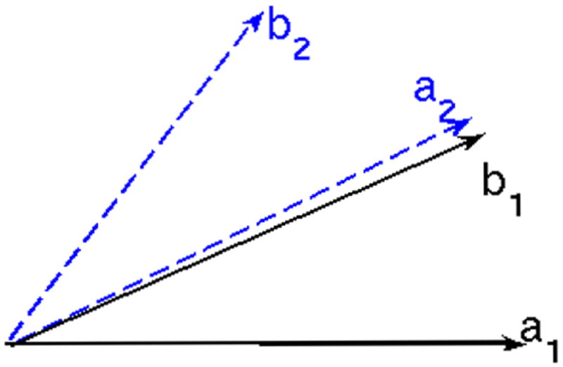
Ambiguity occurs if ordering of the components of mixture model is changed.

In this case, simple calculation can show that the angle between the principal directions of the interpolated result O_t will first decrease and then increase. This is quite unnatural. Thus, to perform correct interpolation, one should always check to make sure that the angle between the principal directions of O_t are either monotonically increasing or decreasing. If this is not the case, make the appropriate change in the ordering of the components of the mixture model.

5. Experiments

5.1. Unimodal Case

In this section, using some synthetic experiments for a 1 tensor model, we compare the representation ability of the directional functions with that of spherical harmonics of a certain order L = 8. In particular, for spherical harmonics, we will use the method given in [11] with the regularizing parameter to compute an ODF. The signals were generated using the model (2) and the true ODF was obtained using (3). We compute the MSE (mean squared error) given by

$$\mathit{MSE}=\frac{1}{N}\sum _{i=1}^N{\left(\frac{\parallel S(i)-\widehat{S(i)}\parallel }{\parallel S(i)\parallel }\right)}^2,$$

where S(i) is the i_th true signal and $\widehat{S(i)}$ is the i^th estimated signal. Rician noise was added to obtain a signal with SNR = 10 dB. 81 gradient directions were used. We also computed the Mean Angle Error (MAE) in degrees for the estimated ODF, which is the average error in the estimation of principal diffusion direction. Note that, typically, the angle error is more when the diffusion directions are very close versus if they are more than 45 degrees apart. For the spherical harmonics, we used a thresholding mechanism to compute the principal directions (ODF maxima) on a tessellation of 642 points on the sphere (where the minimum angle between two adjacent points is 8 degrees).

For the planar case (only the Watson function can be used), we used the following values to generate the signal (2): b = 1000 and eigenvalues of 1e⁻⁶{4000, 4000, 1000}. 1000 samples were generated with random orientation. The MSE between the true signal and estimated signal was 0.1183, while MSE between the corresponding ODF was 0.0242. The MSE for the estimated ODF using spherical harmonics of order 8 was 0.0034.

For the ellipsoidal case, the signal was generated with eigenvalues of 1e⁻⁶{1700, 300, 300} with the same b-value as earlier. The following table gives MSE for 1000 random samples:

For the directional functions the standard deviation of MSE was around 0.0003 while for SH it was 0.0001. It is clear that SH perform better in terms of the MSE whereas the directional functions perform better when finding principal diffusion directions. This is because, the ODF’s computed using SH are much more smooth compared to the directional functions. Note that, one has to use a separate mechanism to find the diffusion directions in the case of SH, whereas with the directional functions, this is already inherent in the model itself.

In the case of MSE, the spherical harmonics use many more coefficients (45 for order l = 8) and hence more degrees of freedom to move the ODF surface, resulting in lower MSE error. For the directional functions, the support is global and only one parameter, the scaling k parameter, really controls the ”shape” of the ODF, thus resulting in slightly more MSE.

5.2. Multi-Modal Case

Assuming two fiber crossings, we used a mixture of two directional functions. 1000 samples were randomly generated with an SNR of 10dB. MSE for this case is listed in the following table:

Once again, the SH does better in terms of the MSE, but performs poorly in terms of estimation of the principal diffusion direction (PDD). We should however note that, we computed the PDD by simple thresholding and that methods such as the one described in [12] could be used for better accuracy. Among the directional functions, the Watson function performs better than the others because of the simple fact that it has a closed form solution for computing the ODF, whereas the other functions are only approximations.

Figure 14, 16 and 17 shows the estimated ODF for real data using all the directional functions with a mixture of 4 components. Although, one could use more components in the mixture, in general, a mixture of 4 gave reasonably good approximations of the measured signal. Thus, we have assumed a maximum of 4 fiber crossings. The data set had 110 gradient directions with a b-value of 1000. The values for γ₁ and γ₂ in equation (15) were empirically chosen to be 0.25 and 1. For SH, an order L = 8 expansion was used. Figure 15 shows a closer view of the rectangular region indicated in Figure 14(a)–(d). Figure 14(f) shows visualization using the GFA scaled min-max normalization of Tuch [37].

Fig. 14.

Estimated ODF for real data with 110 gradient directions. The ROI (genu of the corpus callosum) is taken from the color coded DTI slice shown in (e). In (f), ODF has been visualized using the min-max normalization as given in [37]. A zoomed version of the rectangular region shown in (a)–(d) can be seen in Figure 15.

Fig. 16.

Estimated ODF for real data with 110 gradient directions. The ROI is taken from the color coded DTI axial slice shown in (e). Visualization is done using the min-max normalization and overlayed on the GFA image.

Fig. 17.

Estimated ODF for real data with 110 gradient directions. The ROI is taken from the color coded DTI coronal slice shown in (e). Visualization is done using the min-max normalization and overlayed on the GFA image.

Fig. 15.

Closer view of the rectangular region shown in Figure 14(a)–(d).

The following table gives the mean squared error (MSE) in the estimation of the signal for the real data shown in Figures 14,16,17. Note that, the error computations are for the signal only, since the true ODF is not known. Further, care should be taken in interpreting these results, since lower error does not necessarily imply better estimation since the signal contains measurement noise, which should be removed by a good estimator.

6. Discussion

In this work, we have proposed three different directional functions capable of representing the measured HARDI signals compactly. We have shown a straightforward way to compute their corresponding ODF’s. In particular, the Watson function is capable of representing shapes similar to that of a diffusion tensor but with only 3 coefficients. A generalized measure of anisotropy was also proposed for such a function. In our experiments, we also compared the ability of the Watson function to represent ellipsoidal and planar shapes. Two other directional functions were also presented, namely, the von Mises-Fisher (vMF) and de la Vallee Poussin (dlVP) functions. Based on the error estimates and the fact that there is a nice mathematical formulation of the ODF, the Watson function is a better choice for representing ODFs.

A mixture model was used to represent multimodal ODF’s and a novel energy was proposed to compute the corresponding parameters. We also presented multiple ways to perform interpolation between 2 ODF’s along with formulae to compute geodesic distance in the appropriate spaces. Additionally, we showed the disadvantages of using spherical harmonics for interpolation along with some natural advantages of using directional functions instead. Further, some typical ambiguities that may result while performing interpolation were discussed and solutions were suggested to resolve those.

Nevertheless, there are some open areas of research in the mixture model framework proposed here. First, the estimation of the parameters of the mixture model is slow (around 1 sec per voxel) and necessarily depends on the starting point, thus making it susceptible to local minima. Second, a rigorous analysis of the interpolation techniques proposed in this paper needs to be done. Third, we are working on coming up with a measure of generalized anisotropy for the mixture model, defined only in terms of k, but which is strongly correlated to the measure GFA.

We should also note that, while validation can be easily performed on synthetic data (as was done in this work), there is no established way to validate the results on real data sets (since the ground truth is typically not available), although some work has been done in this direction in [38].

Table 1.

Directional Functions

Function	Signal	ODF
dlVP	B sin2k(θi)	B cos2k(θi)
Watson	C−1 exp(−k cos2 θi)	$C^{-1}exp(-\frac{k}{2}{sin}^2{\theta }_i)$
vMF	A exp(k sin θi)	A exp(k cos θi)

where C = ₁F₁(0.5; 1.5; k), $A=\frac{k}{4\pi \text{sinh}(k)}$ and B are normalization constants.

Table 2.

MSE for unimodal orientation

Function	MSE(signal)	MSE(ODF)	MAE(ODF)
Watson	0.0612	0.0165	7.4 ± 3.1
vMF	0.0758	0.0768	8.3 ± 3.9
dlVP	0.0720	0.0800	8.1 ± 4.2
SH	0.0132	0.0126	10.3 ± 5.8

Table 3.

MSE for multimodal orientation

Function	MSE(signal)	MSE(ODF)	MAE(ODF)
Watson	0.0771	0.0174	8.3 ± 2.9
vMF	0.0852	0.0668	9.1 ± 3.7
dlVP	0.0724	0.0702	13.3 ± 4.1
SH	0.0053	0.0048	18.6 ± 5.2

Table 4.

MSE(signal) for real data

Function	Fig. 14	Fig. 16	Fig. 17
Watson	0.0213	0.0327	0.0405
vMF	0.0295	0.0392	0.0503
dlVP	0.0724	0.0581	0.0568
SH	0.0190	0.0233	0.0259

Appendix A. Anisotropy Measures

Anisotropy measures play an important role in all clinical applications. For a single tensor model, the fractional anisotropy (FA) is widely used. For the multi-fiber case, we use the Generalized Fractional Anisotropy (GFA) measure as defined in [37]:

$$\mathit{GFA}=\frac{\mathit{std}(\text{R}f)}{\mathit{rms}(\text{R}f)}.$$

This measure is quite general and can be used for any model capable of representing ODF’s. There do, however, exist other measures of anisotropy some of which we discuss below.

A.1. Single Tensor Case

Since the Watson function can also be used to model diffusion in a similar way that a single tensor does, we propose a way to compute anisotropy of the single fiber ODF, which is very useful in clinical applications. The anisotropy in (9) only depends on the parameter k. The fractional anisotropy (FA) for single tensor depends on all the three eigenvalues and there is no direct way to relate these with k. We therefore propose a new measure of GFA for the Watson function as follows:

$$GF{A}_w=1-exp(-a\mid k\mid ),$$ (A.1)

where a is a constant. Like FA, this function is guaranteed to be between 0 and 1. The constant a is determined as theminimizer of: || GFA−GFA_w(a) ||² over a typical range of values for k. Figure A.1(a) shows a plot of GFA_w and GFA for a = 1/3.9 which is the optimal value for k ∈ [−10, 20].

Fig. A.1.

(a) Anisotropy measures GFA (dotted line) and GFA_w (solid line). x-axis is range of k. (b) Anisotropy measure −H₂(X) for different values of k.

Alternatively, one could use the Renyi entropy defined as

$$H_{\alpha }(X)=\frac{1}{1-\alpha }log(\sum _{x}P{(x)}^{\alpha })$$

as a measure of anisotropy. Closed-form expression can be obtained for α = 2:

$$\begin{array}{l}{H}_2(X)=-log\left({\int }_0^{2\pi }{\int }_0^{\pi }P{(x)}^{2}sin(\theta )d\theta d\phi \right)\\ =-log\left(\frac{{{}_{1}F}_1(0.5,1.5,2k)}{{{}_{1}F}_1{(0.5,1.5,k)}^2}\right)\end{array}$$ (A.2)

Figure A.1(b) shows a plot of the neg-entropy (−H₂(X)) for various values of k. Although, the range of −H₂(X) does not lie in [0, 1], it gives a good measure of departure from isotropy. For the entropic measure, no parameters have to be chosen (a had to be estimated for computing GFA_w). However, one has to resort to numerical techniques for computing the confluent hypergeometric function in the expression of H₂(X).

In the discussion above, we have only talked about anisotropy measures for theWatson function, since its the only function capable of representing all shapes similar to that of a single tensor.

A.2. Multi-Fiber Case

For the mixture-model representation using dlVP and Watson functions, closed-form solution for negentropy −H₂(X) does not exist. The expression for entropy for the vMF mixture was derived in [26]:

$$H_2(X)=-log\sum _{i=1}^h\sum _{j=1}^h\frac{w_i{w}_j{k}_i{k}_j}{4\pi sinh{k}_{i}sinh{k}_j}\frac{sinh{\rho }_{ij}}{{\rho }_{ij}}$$

where ${\rho }_{ij}=\sqrt{k_i^2+k_j^2+2k_i{k}_j({\mathbf{m}}_i^T{\mathbf{m}}_j)}$.

Further, deriving an expression similar to that of GFA_w for a mixture model is a topic open to research.

Appendix B. Duals of Watson function

There exists a dual for the Watson function (5) introduced earlier. In this dual form, the signal is given by

$$W({\mathbf{u}}_i)=C^{-1}exp\{k{sin}^2{\theta }_i\};{\theta }_i={cos}^{-1}({\mathbf{m}}^T{\mathbf{u}}_i).$$ (B.1)

The approximate ODF can be calculated by a phase shift of π/2 as was discussed earlier:

$$\text{R}W({\mathbf{u}}_i)=C^{-1}exp\{\frac{k}{2}{cos}^2{\theta }_i\}.$$ (B.2)

These functions we call the duals of the Watson function, since they can be alternatively used instead of (5) and (9) to represent the signal and ODF respectively. The main difference in these expressions is a change in the minus sign along with a phase shift of π/2. Note however that, one needs to normalize the duals so that the range of W and RW lies in [0, 1]. The estimation of the parameters m and k stays exactly the same as was done for the Watson function.

References

- 1.Alexander D. Maximum entropy spherical deconvolution for diffusion MRI. Information Processing in Medical Imaging. 2005:76–87. doi: 10.1007/11505730_7. [DOI] [PubMed] [Google Scholar]
- 2.Alexander D, Barker G, Arridge S. Detection and modeling of nongaussian apparent diffusion coefficient profiles in human brain data. Magnetic Resonance in Medicine. 2002;48:331–340. doi: 10.1002/mrm.10209. [DOI] [PubMed] [Google Scholar]
- 3.Amari S, Nagaoka H. Methods of information geometry. AMS; 2000. [Google Scholar]
- 4.Assemlal H-E, Tschumperlé D, Brun L. A variational framework for the robust estimation of odfs from high angular resolution diffusion images. 2007 April 1; [Google Scholar]
- 5.Banerjee A, Dhillon I, Gosh J, Sra S. Clustering on the unit hypersphere using von Mises-Fisher distributions. Journal of Machine learning Research. 2005;6:1345– 1382. [Google Scholar]
- 6.Basser P, Pajevic S. A normal distribution for tensor-valued random variables: applications to diffusion tensor MRI. IEEE Trans on Medical Imaging. 2003;22:785–794. doi: 10.1109/TMI.2003.815059. [DOI] [PubMed] [Google Scholar]
- 7.Bergmann O, Kindlmann G, Lundervold A, Westin C-F. Diffusion k-tensor estimation from q-ball imaging using discretized principal axes. MICCAI. 2006:268–275. doi: 10.1007/11866763_33. [DOI] [PubMed] [Google Scholar]
- 8.Bhalerao A, Westin C-F. Hyperspherical von Mises-Fisher mixture modeling of high angular resolution diffusion mri. MICCAI. 2007;4791:236–243. doi: 10.1007/978-3-540-75757-3_29. [DOI] [PubMed] [Google Scholar]
- 9.Chen Y, Guo W, Zeng Q, Yan X, Huang F, He G, Vemuri B, Liu Y. Estimation, smoothing and characterization of apparent diffusion coefficient profiles from high angular resolution DWI. CVPR. 2004:588–593. [Google Scholar]
- 10.Descoteaux M, Deriche R. Segmentation of Q-ball images using statistical surface evolution. MICCAI. 2007;4792:769–776. doi: 10.1007/978-3-540-75759-7_93. [DOI] [PubMed] [Google Scholar]
- 11.Descoteaux M, Angelino E, Fitzgibbons S, Deriche R. Regularized, fast and robust analytical q-ball imaging. Magnetic Resonance in Medicine. 2007;58(3):497– 510. doi: 10.1002/mrm.21277. [DOI] [PubMed] [Google Scholar]
- 12.Descoteaux M, Deriche R, Anwander A. Deterministic and probabilistic q-ball tractography: from diffusion to sharp fiber distributions. Technical Report 6273; INRIA Sophia Antipolis. August 2007. [Google Scholar]
- 13.Friman S, Peled O, Jolesz F, Westin C-F. Geometrically constrained tw-tensor model for crossing tracts in dwi. Magnetic Resonance in Medicine. 2006;24(9):1263– 1270. doi: 10.1016/j.mri.2006.07.009. [DOI] [PMC free article] [PubMed] [Google Scholar]
- 14.Ghosh A, Descoteaux M, Deriche R. Riemannian framework for estimating symmetric positive definite 4th order diffusion tensor. MICCAI. 2008:858–865. doi: 10.1007/978-3-540-85988-8_102. [DOI] [PubMed] [Google Scholar]
- 15.Jansons K, Alexander D. Persistent angular structure: New insights from diffusion magnetic resonance imaging data. Inverse Problems. 2003;19:1031–1046. [Google Scholar]
- 16.Jian B, Vemuri B. A unified computational framework for deconvolution to reconstruct multiple fibers from diffusion weighted MRI. IEEE Trans on Medical Imaging. 2007;26(11):1464–1471. doi: 10.1109/TMI.2007.907552. [DOI] [PMC free article] [PubMed] [Google Scholar]
- 17.Jupp P, Mardia K. A unified view of the theory of Directional Statistics. International Statistical Review. 1989;57:261–294. [Google Scholar]
- 18.Kaden E, Anwander A, Knsche T. Parametric spherical deconvolution: Inferring anatomical connectivity using diffusion MR imaging. Neuroimage. 2007;37:477–488. doi: 10.1016/j.neuroimage.2007.05.012. [DOI] [PubMed] [Google Scholar]
- 19.Kaden E, Anwander A, Knsche T. Variational inference of the fiber orientation density using diffusion MR imaging. Neuroimage. 2008;42(4):1366–1380. doi: 10.1016/j.neuroimage.2008.06.004. [DOI] [PubMed] [Google Scholar]
- 20.Khachaturian M, Wisco J, Tuch D. Boosting the sampling efficiency of q-ball imaging using multiple wavevector fusion. Magnetic Resonance in Medicine. 2007;57:289–296. doi: 10.1002/mrm.21090. [DOI] [PubMed] [Google Scholar]
- 21.Kubicki M, McCarley RW, Westin CF, Park HJ, Maier S, Kikinis R, Jolesz FA, Shenton ME. A review of diffusion tensor imaging studies in schizophrenia. Journal of Psychiatry Research. 2005;41:15–30. doi: 10.1016/j.jpsychires.2005.05.005. [DOI] [PMC free article] [PubMed] [Google Scholar]
- 22.leow A, Zhu S, McMohan K, Zubicaray G, Meredith M, Wright M, Thompson P. Probabilistic multi-tensor estimation using the tensor distribution function. CVPR. 2008:1–6. [Google Scholar]
- 23.Lin C, Wedeen V, Chen J, Yao C, Tseng W. Validation of diffusion spectrum magnetic resonance imaging with manganese-enhanced rat optic tracts and ex vivo phantoms. Neuroimage. 2003;19:482–495. doi: 10.1016/s1053-8119(03)00154-x. [DOI] [PubMed] [Google Scholar]
- 24.Liu C, Bammer R, Acar B, Moseley M. Characterizing non-gaussian diffusion by using generalized diffusion tensors. Magnetic Resonance in Medicine. 2004;51:924–937. doi: 10.1002/mrm.20071. [DOI] [PubMed] [Google Scholar]
- 25.McGraw T, Vemuri B, Yezierski B, Mareci T. Von mises-fisher mixture model of the diffusion ODF. ISBI. 2006:65–68. doi: 10.1109/ISBI.2006.1624853. [DOI] [PMC free article] [PubMed] [Google Scholar]
- 26.McGraw T, Vemuri B, Yezierski B, Mareci T. Segmentation of high angular resolution diffusion MRI modeled as a field of von Mises-Fisher mixtures. ECCV. 2007:461–475. [Google Scholar]
- 27.Ozarslan E, Mareci T. Generalized diffusion tensor imaging and analytical relationships between diffusion tensor imaging and high angular resolution imaging. Magnetic Resonance in Medicine. 2003;50:955–965. doi: 10.1002/mrm.10596. [DOI] [PubMed] [Google Scholar]
- 28.Ozarslan E, Shepherd T, Vemuri B, Blackband S, Mareci T. Resolution of complex tissue microarchitecture using the diffusion orientation transform (dot) Neuroimage. 2006;31:1083–1106. doi: 10.1016/j.neuroimage.2006.01.024. [DOI] [PubMed] [Google Scholar]
- 29.Parker G, Alexander D. Probabilistic monte carlo based mapping of cerebral connections utilising wholebrain crossing fibre information. Information Processing in Medical Imaging. 2003;18:684–695. doi: 10.1007/978-3-540-45087-0_57. [DOI] [PubMed] [Google Scholar]
- 30.Alonso Ramirez-Manzanares, Philip Cook, James Gee. A comparison of methods for recovering intra-voxel white matter fiber architecture from clinical diffusion imaging scans. MICCAI. 2008;1:305–312. doi: 10.1007/978-3-540-85988-8_37. [DOI] [PubMed] [Google Scholar]
- 31.Schaeben H. A simple standard orientation density function: The hyperspherical de la Vallee Poussin kernel. Physica Status Solidi (B) 1997;200:367–376. [Google Scholar]
- 32.Schaeben H, Hielscher R, Funderburger J, Potts D, Prestin J. Orientation density function-controlled pole probability density function measurements: automated adaptive control of texture goniometers. Journal of Applied Crystallography. 2007;40:570–579. [Google Scholar]
- 33.Tournier J, Calamante F, Gadian D, Connelly A. Direct estimation of the fiber orientation density function from diffusion-weighted mri data using spherical deconvolution. Neuroimage. 2004;23:1176–1185. doi: 10.1016/j.neuroimage.2004.07.037. [DOI] [PubMed] [Google Scholar]
- 34.Tournier J-D, Yeh C, Calamante F, Cho H, Connelly A, Lin P. Resolving crossing fibres using constrained spherical deconvolution: validation using diffusion-weighted imaging phantom data. Neuroimage. 2008;41:617–625. doi: 10.1016/j.neuroimage.2008.05.002. [DOI] [PubMed] [Google Scholar]
- 35.Tuch D, Reese T, Wiegella M, Makris N, Belliveau J, Wedeen V. High angular resolution diffusion imaging reveals intravoxel white matter fiber heterogeneity. Magnetic Resonance in Medicine. 2002;48:577–582. doi: 10.1002/mrm.10268. [DOI] [PubMed] [Google Scholar]
- 36.Tuch D, Reese T, Wiegell M, Wedeen V. Diffusion MRI of complex neural architecture. Neuron. 2003;40:885–895. doi: 10.1016/s0896-6273(03)00758-x. [DOI] [PubMed] [Google Scholar]
- 37.Tuch David S. Q-ball imaging. Magnetic Resonance in Medicine. 2004;52:1358–1372. doi: 10.1002/mrm.20279. [DOI] [PubMed] [Google Scholar]
- 38.Zhan W, Yang Yihong. How accurately can the diffusion profiles indicate multiple fiber orientations ? A study on general fiber crossings in diffusion MRI. Journal of Magnetic Resonance. 2006;183:193–202. doi: 10.1016/j.jmr.2006.08.005. [DOI] [PubMed] [Google Scholar]