Local RNA structure alignment with incomplete sequence

Abstract

Motivation: Accuracy of automated structural RNA alignment is improved by using models that consider not only primary sequence but also secondary structure information. However, current RNA structural alignment approaches tend to perform poorly on incomplete sequence fragments, such as single reads from metagenomic environmental surveys, because nucleotides that are expected to be base paired are missing.

Results: We present a local RNA structural alignment algorithm, trCYK, for aligning and scoring incomplete sequences under a model using primary sequence conservation and secondary structure information when possible. The trCYK algorithm improves alignment accuracy and coverage of sequence fragments of structural RNAs in simulated metagenomic shotgun datasets.

Availability: The source code for Infernal 1.0, which includes trCYK, is available at http://infernal.janelia.org

Contact: kolbed@janelia.hhmi.org; eddys@janelia.hhmi.org

Supplementary information: Supplementary data are available at Bioinformatics online.

1 INTRODUCTION

Sequence alignment approaches may be broadly divided into global alignment methods, where sequences are assumed to be homologous and alignable over their entire lengths, and local alignment methods, where only part of each sequence is assumed to be homologous and alignable (Durbin et al., 1998; Gusfield, 1997). Local alignment is more widely used because there are many biological and technical reasons why sequences may not be globally alignable. For example, many protein sequences have arisen by accretion of common protein domains in different combinations (Vogel et al., 2004), and some high-throughput sequencing strategies such as metagenomic shotgun sampling generate fragmentary sequence data (Schloss and Handelsman, 2005).

For local alignment of primary sequences (Altschul et al., 1990; Pearson and Lipman, 1988; Smith and Waterman, 1981), one is merely looking for an alignment of contiguous linear subsequences of a query and a target. At this level, there is little informative difference between local alignments that arise by biological evolution versus incomplete data. However, the nature of local alignment can be markedly different when we adopt more realistic and complex sequence alignment models that capture evolutionary constraints at a higher level than primary sequence alone. For example, in comparing 3D protein structures, which often share structural similarity in only part of their overall fold (Chothia and Lesk, 1986), it is advantageous to adopt local structural alignment algorithms that allow alignment of spatially local units of 3D structure that may not be composed of contiguous colinear residues in the primary sequence (Gibrat et al., 1996).

Here we are concerned with alignment of structural RNAs, using models that consider both primary sequence and secondary structure constraints. Evolution of a structural RNA is constrained by its secondary structure. Base pairing tends to be conserved even as the sequence changes, and aligned sequences exhibit correlated substitutions in which base pairs are substituted by compensatory base pairs. Computational methods for aligning structural RNAs under a combined primary sequence and secondary structure scoring model have been developed (Backofen and Will, 2004; Sakakibara et al., 1994) including ‘covariance model’ (CM) [profile stochastic context-free grammar (SCFG)] methods (Durbin et al., 1998; Eddy, 2002; Eddy and Durbin, 1994; Nawrocki and Eddy, 2007). These models represent a given RNA consensus secondary structure as a binary tree, with individual nodes representing and scoring individual base pairs and single-stranded residues.

Local RNA secondary structural alignment has been implemented by allowing an alignment to start or end at any internal node in the tree (Backofen and Will, 2004; Eddy, 2002; Klein and Eddy, 2003), much as local primary sequence alignment allows starting and ending at any residue in the linear sequence. This subtree method of local RNA alignment can include or exclude any subtree of the RNA, corresponding well to secondary structure domains. Biologically, this serves as a reasonable approximation of some important evolutionary constraints on RNA secondary structure alignment, although it neglects higher order constraints, including pseudoknots and tertiary structure.

However, defining locality by subtrees is a poor model of local structural RNA alignment when locality arises for technical rather than biological causes. A shotgun sequencing strategy will truncate at the linear sequence level without respect for the conserved base-paired structure, and residues involved in base pairs may be missing in the observed sequence, as illustrated in Figure 1. In this case, we do not want to score the missing residues as deletions of conserved base pairs, but neither do we want to leave the homologous observed residues unaligned if we are trying to get the most information from fragmentary sequence data.

Fig. 1.

Comparison of local alignment types. Left: global alignment; filled circles indicate observed residues in an RNA structure, which can be thought of as a binary tree. Center: subtree method of local RNA structural alignment. Whole domains of the RNA structure may be skipped (open circles indicate consensus positions without aligned sequence residues), but the observed alignment satisfies all expected structural constraints: if a residue is aligned to a pair state, another residue will be aligned to form a base pair. Right: truncated sequence method of local RNA structural alignment, where the observed sequence may begin and end anywhere with respect to the consensus RNA structure. Aligned residues may be base-paired to positions that are missing from the alignment.

Here, we will focus specifically on the homology search and alignment problem. We have a given RNA sequence and secondary structure as a query, and the task is to search a sequence database for homologous sequences and/or align target sequences to the query. This is directly analogous to the use of the Smith/Waterman local alignment algorithm for primary sequence analysis (Smith and Waterman, 1981), and it is the problem addressed by our Infernal software package (E. P. Nawrocki et al., 2009), for instance using Rfam models of known RNA families to infer and annotate homologous RNAs in genome sequence (Gardner et al., 2009). It should not be confused, for example, with the related problem of de novo motif identification, which arises in RNA analysis when the input data consist of two or more sequences that are presumed to share an unknown structural motif in common, and the task is to produce a local structural alignment that identifies the common motif and infers its common structure. De novo motif identification requires a means of inferring the unknown structural consensus in addition to a local alignment algorithm. Although we expect that de novo motif identification approaches such as CMFinder (Yao et al., 2006) or other approaches for inferring locally conserved RNA structure such as LocARNA (Will et al., 2007) would be able to incorporate the local alignment algorithm we will describe, for the purposes of introducing our local alignment algorithm in the present article, we will not discuss the de novo motif identification problem further.

An important example of the local RNA alignment problem in homology search and alignment arises in metagenomic shotgun survey sequencing (Chen and Pachter, 2005; Schloss and Handelsman, 2005), particularly when assembly is incomplete or not possible. Structural RNA sequence alignments (particularly of small subunit ribosomal RNA) are important in analyzing the phylogenetic diversity of metagenomic samples, but a single shotgun read (often of only about 200–400 bp) will fall more or less randomly into the consensus alignment of an RNA, generally leaving unsatisfied consensus base pairs because of the incomplete nature of the sampled sequences, and it may also include extraneous genomic sequence.

To deal with this truncated sequence type of locality, we want to align the observed sequence, or a subsequence of it, to a contiguous subsequence of the yield of the model's tree: the linear consensus sequence, as read counterclockwise around the tree's leaves. We want to use secondary structure information wherever we have both residues in a base pair, but revert to primary sequence alignment when we are missing sequence data. If we magically knew a priori the endpoints of the correct alignment of an observed sequence read with respect to the yield of the RNA model, we could derive a new model that used base-pair states where we had both residues, and converted pair states to appropriately marginalized single-residue states where the pairing partner was missing. The problem is that these endpoints must be inferred when we align the observed sequence to the model. We describe an optimal recursive dynamic programming solution for this problem, and evaluate the algorithm's utility in accurate alignment of simulated datasets of unassembled metagenomic sequence.

2 APPROACH

2.1 Local alignment as a missing data problem

We frame the alignment of truncated sequences as a missing data inference problem (Rubin, 1976). We specify two probabilistic processes: one that generates complete data (our existing probabilistic model of global alignment), and one that generates observed fragments from the complete data (by random sequence truncation). The joint probability of observed sequence fragments and their local alignment to the model will then be an appropriate marginal sum over global alignments. We will identify the optimal local alignment for the observed sequence by maximizing this joint probability.

We will describe the essence of the approach (and two approximations we make) in general terms with respect to binary trees, deferring the specific notation we use for profile SCFGs (CMs). In a CM, both the consensus structure of the model and a particular structural alignment of the model to an individual RNA sequence are binary trees. [A binary tree suffices to capture all nested base-pairing correlations, but non-nested interactions such as pseudoknots and higher order interactions such as base triples are neglected (Durbin et al., 1998).] Construction of a CM starts by representing the RNA consensus structure as a ‘guide tree’, with ‘nodes’ representing consensus base pairs and consensus unpaired positions. Each consensus node is then stereotypically expanded into one or more SCFG ‘states’, with one state representing the consensus (‘match’) behavior and additional states and state transitions representing the probability of insertions and deletions relative to consensus. A CM is a special case of SCFGs, with all its states and state transitions arranged in a directed graph following the branching pattern of a consensus RNA structure's binary tree. An alignment of the CM to a particular sequence is represented as an SCFG parse tree, a state path through the consensus guide tree, using match, insert and delete states to account for alignment positions, and start, bifurcation and end states to account for the branching tree structure itself.

A parameterized RNA CM θ specifies a joint probability distribution over complete sequences and parse trees : i.e. over global alignments.

A missing data process specifies how a complete sequence with length is truncated to an observed sequence fragment x of length L, and correspondingly, how the global parse tree is truncated to a notion of a local parse tree π. (We will solidify our definition of a local parse tree shortly.) Because we are imagining a complete sequence randomly truncated to a sequence fragment, the missing data process would ideally be conditionally independent of the model and the parse tree. For instance, we could sample each possible sequence fragment from a complete sequence of length with uniform probability . However, under this missing data process, we would need to marginalize (sum over) all possible complete sequences of all possible lengths . This term becomes problematic in the recursive dynamic programming optimization framework we describe below.

Instead, we will make what should be a reasonable approximation of the truncation process. We assume that a truncation Δ^gh is done by selecting a fragment g…h relative to the positions in the fixed-length consensus yield as defined by the model (the consensus sequence positions defined by the CM's consensus guide tree nodes). This truncation is then conditionally independent of both the parse tree and the sequence. This approximation should be reasonable because high-probability complete sequences will generally have lengths similar to the consensus length. It means that local alignments will only begin and end at consensus positions, never at sequence insertions. For a model with W consensus positions, the probability of choosing any particular fragment g…h with respect to the complete yield 1..W is P(Δ^gh∣θ)=2/(W(W+1)). This term is now a constant with respect to the necessary summation over complete data.

Now we define what we mean by a local parse tree fragment π. Choose two positions g, h on the consensus yield of the model: these consensus sequence positions correspond unambiguously to states s_g and s_h in parse trees (the states used by the parse tree to account for how the endpoints of a particular sequence align to a model consensus position: either a consensus match, or a deletion). A ‘local parse tree’ π^gh (equivalent to what we have called just π until now) is defined as the minimal (smallest) subtree of a complete parse tree that contains s_g and s_h. Usually, this is a parse subtree rooted at either s_g or s_h, but s_g and s_h may also be on opposing sides of a bifurcation, with the minimal subtree rooted at the bifurcation state.

Truncation of a complete parse tree to a local parse tree π^gh defines two different sorts of missing data. Outside the local parse tree, we are missing (and will sum over) both sequence residues and parse tree states that were in the complete parse tree; let this missing data be represented by x′, π′. Inside the local parse tree, we may have states with unsatisfied, missing sequence residues, such as base pairs where only one residue is in the observed sequence: here, we will be summing only over the missing sequence residues, denoted as x″. The combination of the observed data (x, π^gh) and the unobserved data (x″, x′, π′) together uniquely determine the complete alignment .

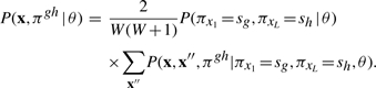
The desired joint probability may then be written as a summation over the two types of missing data defined by a local parse tree:

Summation over missing data x′, π′ results in two terms. The first is a term P(π_x1=s_g, π_xL=s_h∣θ) that represents the marginal probability that a complete parse tree truncated at g, h has states s_g, s_h assigned to the endpoints of the truncation; this is just the fraction of complete parse trees that contain states s_g and s_h. The second term is P(x, x″, π^gh∣π_x1=s_g, π_xL=s_h, θ) for the local parse tree and its associated sequence residues (both observed and unobserved) conditional on local parse tree endpoints at states s_g, s_h. Thus

Although it is straightforward to calculate P(π_x1=s_g, π_xL=s_h∣θ), the term becomes problematic in the dynamic programming recursion we define. One or both of the optimal truncation endpoints s_g, s_h are undetermined until the dynamic programming recursion is complete and a traceback is performed. We therefore make our second approximation here, approximating this term as 1.0 when s_g, s_h are consensus match states and 0.0 when they are not. This corresponds to an assumption that all probability mass flows through the consensus match states at the endpoints g, h, neglecting the probability that an SCFG deletion state could be used at one of these consensus positions. Local alignments will therefore be forced to start and end with consensus match positions (just as in standard Smith/Waterman local sequence alignment). This leaves

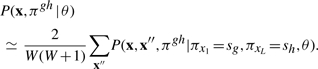In Section 2.2, we show there is an efficient dynamic programming algorithm for finding the parse tree π^gh that performs the necessary summation over missing data and maximizes this joint probability for a given observed sequence fragment x.

2.2 Description of the trCYK algorithm

The Cocke–Younger–Kasami (CYK) algorithm is a standard algorithm for calculating the maximum likelihood SCFG parse tree for a given sequence (Durbin et al., 1998; Hopcroft and Ullman, 1979; Kasami, 1965; Younger, 1967). CYK recursively calculates terms α_v(i, j) representing the log probability of the optimal parse subtree rooted at state v that accounts for a subsequence x_i …x_j, initializing at the smallest subtrees and subsequences (model end states aligned to subsequences of length 0) and iteratively building larger subtrees accounting for longer subsequences. At termination, the score α₀(1, L) is the log probability of a parse tree rooted at the model's start state 0 accounting for the complete sequence x₁ …x_L. The optimal parse tree is then recovered by a traceback of the dynamic programming matrix. When applied specifically to a CM of M consensus nodes and a sequence of length L, the CYK algorithm requires O(L²M) memory and O(L³M) time (Eddy and Durbin, 1994). A more complex divide-and-conquer variant of the CM CYK algorithm requires O(L²logM) memory (Eddy, 2002).

Previously, we implemented subtree-based local RNA structure alignment by a minor adaptation of the CM's generative model that required no substantive alteration of the CYK algorithm. Specifically, we allowed a start transition from the model's root state 0 to any of the consensus states in the model, and we allowed an end transition from any consensus state in the model to a ‘local end’ (EL) state that emits zero or more non-homologous residues with a self-transition loop. The start transition allows the model to align to any model subtree and not just the complete model, and the end transition allows it to replace any subtree with a non-homologous insertion.

The truncated sequence local alignment algorithm we describe here, for finding an optimal local parse tree π^gh that accounts for a linear sequence fragment, does require a substantial modification of the CYK algorithm because it needs to identify the optimal endpoints g, h. The two approaches to local alignment are not mutually exclusive. We retain the local end transition to an EL state to model non-homologous replacement of structural elements inside a local parse subtree.

The key property of local parse trees π^gh that enables a recursive CYK-style algorithm can be summarized as ‘once marginal, always marginal’, as illustrated in Figure 2. As the CYK calculation builds larger and larger subtrees—climbing ‘up’ the model—it will usually grow by adding appropriate (v, i, j) triplets that deal with complete (joint) emission of any base-paired residues (upper left panel of Fig. 2). At some point, it may need to decide that the sequence is truncated at either the right or left endpoint of the optimal parse subtree (upper middle and upper right panels of Fig. 2, respectively), in which case only the left residue x_i or the right residue x_j (respectively) will be added to the growing parse subtree, and scored as the marginal probability of generating the observed residue at state v summed over all possible identities of the missing residue. We refer to this as ‘joint mode’ versus left and right ‘marginal modes’ for a growing alignment. The switch from joint mode to a marginal mode identifies one of the endpoints (h or g, respectively). Once switched, the alignment must stay in that marginal mode until the root state of the optimal local parse subtree is identified. Left marginal mode alignments may only be extended by aligning left residues x_i (central panel of Fig. 2), and right marginal mode alignments may only be extended by aligning right residues x_j (center right panel of Fig. 2). In marginal modes, residue emission probabilities involving missing data are the appropriate marginal summation of the state's emission probabilities.

Fig. 2.

Extension possibilities for building alignments. Extension may generally be joint (J), left marginal (L) or right marginal (R). Top: an existing joint alignment may use any type of extension. Grey circles indicate the previously existing alignment, with the new residues added in red, and open circles for when no residue is aligned. Transitioning from joint to marginal alignment sets an endpoint of the alignment. Center: an alignment that is already marginal may only continue with marginal extension on the same side. Bottom: a new alignment may be started in any of the three modes. The joint alignment here is shown skipping a portion of the subtree, but that need not be the case. Initiating an alignment in marginal mode also sets one of the alignment endpoints.

In order to recursively calculate the optimal local parse tree, including these optimal switch points from joint to marginal modes, we extend the CYK algorithm to treat the different modes separately (essentially as an additional layer of hidden-state information), and calculate separate matrices for each mode: α^J for the standard case (joint mode), α^L for extension only at the 5′ end (emissions are marginalized to the left) and α^R for extension only at the 3′ end (emissions are marginalized to the right). Each column in Figure 2 illustrates the main cases that have to be examined: for example, the calculation of α^L_v(i, j) for a base-pair emitting state v would examine each of its transition-connected states y and consider both the possibility of reaching (v, i, j) by extension of a previously calculated left-marginal α^L_y(i−1, j), and the possibility of reaching it by switching from a previously calculated joint α^J_y(i−1, j).

The calculation at bifurcation states requires special consideration, as illustrated in Figure 3. Only combinations of modes for left and right branches that would form a contiguous subsequence x_i …x_j aligned to a local parse tree rooted at bifurcation state v are allowed. Cases in which an entire branch is missing data must also be considered (shown as ∅ in Fig. 3). There is a unique case when both branches of the bifurcation have marginal alignments (bottom of Fig. 3), and the resulting join cannot be extended further. For convenience, we call the score of this case α^T, noting that it is only defined when v is a bifurcation state and that because it is a terminal case, it does not have to be stored in the recursion.

Fig. 3.

Extension possibilities at bifurcations. A bifurcation state joins two subtrees, one 5′ (left, blue) and one 3′ (right, red). Each subtree has its own alignment mode, either joint (J), left marginal (L), right marginal (R), or empty (∅). The subtree modes together must give a continuous subsequence, and all valid combinations are shown. The combination determines the mode of the bifurcation state, which can subsequently be extended like any other state, except for the terminal case T. (Arrows show possibilities for later extension.)

The score of the optimal local parse tree aligned to a subsequence x_i …x_j is the combination of consensus state v, sequence positions i, j and mode X∈{J, L, R, T} that maximizes α^X_v(i, j). Alternatively, the entire observed sequence x₁ …x_L can be forced into an optimal local alignment to the model by choosing v, X that maximize α^X_v(1, L).

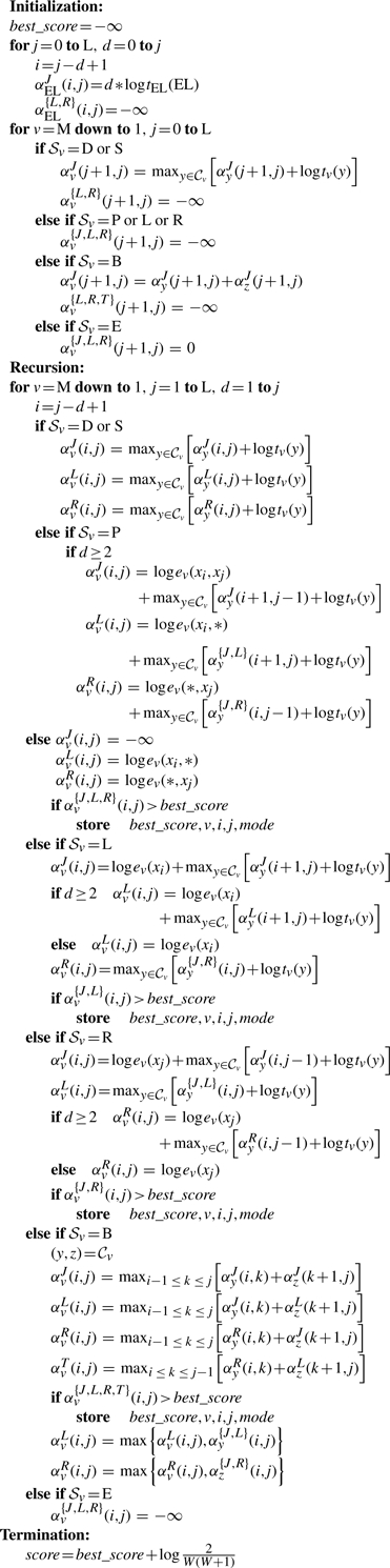
2.3 The trCYK algorithm

The following description of the truncated sequence CYK dynamic programming algorithm (trCYK) assumes familiarity with notation and conventions used in previously published descriptions of CMs (Durbin et al., 1998; Eddy, 2002). Briefly, sequence positions are indexed by i, j and k; x_i is the residue at position i; and d refers to the length of a subsequence x_i …x_j where d=j−i+1. The main parameters of a CM are the emission and transition probabilities of its states. These states are indexed by v, y, z, ranging from 1 to M, the total number of model states. 𝒞_v lists all the children y of state v; the transition probability for moving from v to y is t_v(y). (A bifurcation state v splits to y, z with probability 1.0.) 𝒮_v is the type of state v; possible values are S (start), P (pair emit), L (left emit), R (right emit), D (deletion), B (bifurcation) and E (end). The e_v represents emission probabilities at state v, which (depending on the state type) may emit either one or two residues, e_v(x_i)) or e_v(x_i, x_j). Emission probabilities marginalized over a missing residue are indicated by a ‘*’ for the missing residue; for example e_v(x_i, *)=∑_ae_v(x_i, a).

After this recursion is completed, the optimal local parse tree may be recovered by traceback from the best scoring α^X_v(i, j). To facilitate this, it is helpful to store traceback pointers during the dynamic programming recursion; for clarity, these are not indicated in the algorithm description above. In order to avoid parsing ambiguity, any ties in the traceback are resolved in favor of joint mode over marginal modes. Thus, marginal mode is only used when required to account for one or more missing residues in the local parse tree.

It is worth noting that an additional kind of structural alignment locality is dealt with by the state structure of a CM, rather than by the trCYK algorithm. The alignable subsequence (as identified by trCYK) may also be subject to large internal deletions and insertions relative to the consensus RNA structure. CMs accomodate large structural insertions and deletions by allowing any consensus state to transition to a special EL state which has a self-transition loop, thereby allowing any structural domain to be truncated anywhere and replaced by zero or more non-homologous residues. The EL state appears in the recursion above, and its use and rationale for accomodating local structural variation are more fully explained elsewhere (Klein and Eddy, 2003).

3 IMPLEMENTATION

The algorithm described above requires O(L²M) memory to store traceback pointers for recovering an optimal local parse tree. In order to be able to align large RNAs, we also implemented an extension of the divide and conquer approach described in (Eddy, 2002) to trCYK, reducing the memory requirement to O(L²logM) at the expense of a small increase in computation time. The divide and conquer version was used to obtain the results described below. Both versions are provided in the ANSI C source code of Infernal in the Supplementary Material.

The trCYK has an upper bound time complexity of O(L³M), the same as standard CYK. The trCYK's additional calculations and three matrices in place of one contribute a constant multiplier. Empirically, trCYK runs about 5-fold slower than standard CYK on the same problem size. For example, a single RNase P alignment for the results in Figure 2 (283 nodes and 1119 states in the model; sequence length of 400) took 40 s for trcyk vs. 9.4 s for Infernal cmsearch with equivalent settings, on a single 3.0 GHz Intel Xeon processor.

4 EVALUATION

We compared the effectiveness of the trCYK method for local structural RNA alignment with the previous subtree method, by measuring how accurately and completely the two methods align single shotgun sequence reads to structural RNA consensus models. To do this, we constructed a synthetic test of realigning simulated reads generated by sampling sequence fragments from trusted (presumed correct) alignments. We chose to use simulated data instead of real data because we are interested in conducting a controlled comparison of the two algorithms against known correct answers. Because alignment quality and (in particular) local alignment coverage are strongly affected by parameterization, in order to isolate the algorithm's effect, we used the same profile SCFGs as parameterized by the same implementation (Infernal), and compared Infernal's default subtree alignment method versus its newly implemented trCYK option. To put this comparison in context, we also test two other primary sequence methods: pairwise alignment with BLASTN, and sequence profile alignment with HMMER.

We used multiple sequence alignments of two well known structural RNA genes, small subunit ribosomal RNA (SSU rRNA) and RNase P. SSU rRNA is in general highly conserved, so in many regions of the RNA consensus and for all but the most outlying taxa, SSU rRNA is usually not a particularly challenging sequence alignment problem. RNase P sequences, in contrast, tend to be highly divergent at the primary sequence level. For a trusted RNase P multiple alignment, we used the bacterial class A seed alignment from Rfam 8.1 (Brown, 1999; Griffiths-Jones et al., 2005), and our trusted SSU rRNA alignment was adapted from the bacterial seed alignment from the Comparative RNA Web (CRW) site, (Cannone et al., 2002). Due to the large number of sequences, the SSU alignment was filtered to remove sequences such that no aligned pair was >92% pairwise identical. It was also edited slightly towards a consensus structural alignment in preference to an evolutionarily correct alignment where there was ambiguity between structural conservation and homology. Our SSU rRNA alignment is provided in the Supplementary Material.

The sequences in the trusted alignment were clustered by single linkage by pairwise identity (as defined by the original alignment) and split into a smaller training alignment subset and a testing set, so as to minimize pairwise identity between training and test data and create more challenging alignment tests. For SSU, this gave 101 training sequences and 51 testing sequences, with maximum identity between sets of 82%. The smaller RNase P family has 28 training sequences and 15 testing sequences, with maximum identity of 60%.

We simulated a genomic context for each test sequence, consisting of randomly generated sequence of the same monoresidue composition, and then sampled a random subsequence of length 800 (SSU rRNA) or 400 (RNase P) that contained at least 100 nucleotides of the RNA. Five fragments were sampled for each SSU rRNA test sequence, and 10 for each RNase P test sequence, for a total of 255 SSU test fragments and 150 RNase P test fragments. The 800 nt length of SSU rRNA test fragments roughly corresponds to the average single read length in recent metagenomic sequencing surveys with Sanger sequencing technology (Rusch et al., 2007; Venter et al., 2004). RNase P is a shorter RNA (average length just 310 nt) so shorter fragments of 400 bases were used, roughly according to the current capabilities of newer 454 sequencing technology. The training alignments and test fragments are provided in the Supplementary Material.

We aligned each test sequence fragment to the training alignment using four different local alignment methods. For BLAST local sequence alignment, we used NCBI BLASTN (Altschul et al., 1997), with default parameters except for a word length of W=6 and an E-value cut-off of 1.0, and used the pairwise alignment with the lowest E-value to identify the nearest neighbor among any of the individual training set sequences. All alignments to that nearest neighbor, including lower scoring ones, were considered as portions of the complete alignment. For profile alignment, we used HMMER 2.3.2 (Eddy, 2008) to build a profile HMM from the training alignment subset with hmmbuild using the -f option to build local alignment models, and aligned each test fragment to the profile (thereby adding it to the multiple alignment with the training sequences) with hmmalign using default parameters. For the subtree-based local alignment method, we used Infernal version 1.0 to build a CM of the training alignment subset with cmbuild with the –enone option to shut off entropy weighting. [We have observed that Infernal's entropy weighting option (Nawrocki and Eddy, 2007) is appropriate for maximal sensitivity in remote homology search, but not for alignment accuracy; D.L.K., S.R.E. and E. Nawrocki, unpublished data.] We aligned each test fragment to the CM with cmsearch using default parameters. Finally, for trCYK, we used the trcyk program included in Infernal 1.0 to align test fragments to the same CM used for cmsearch.

To evaluate the alignments, they are mapped to the reference alignment using an intermediary sequence; for BLASTN, this is the nearest neighbor sequence it was aligned to, and for the profile methods it is the consensus sequence of the model. If a residue in the test sequence was aligned to a non-gap position in the reference alignment, it is correct in the output alignment if it is aligned to that same position, and incorrect otherwise. If the residue was originally aligned to a gap position, it is judged to be correct if, in the output alignment, it is between the same two consensus positions that bordered the original gap. Misaligned residues include both residues that should be aligned but are incorrect, and residues that should not be aligned at all (part of the surrounding ‘genomic’ sequence). We measured both the accuracy of the resulting alignments [positive predictive value (PPV): the fraction of aligned positions that are also found in the trusted alignment] and the coverage (sensitivity: the fraction of aligned positions in the trusted alignment that are found in the calculated local alignment).

The results, mean and standard deviations for sensitivity and PPV for each method, are shown in Figure 4. BLAST generally returns highly accurate alignments, but has low coverage, corresponding to a tendency to pick out only the most highly conserved portions of the true alignments. (The default NCBI BLAST scoring scheme is tuned for high sequence identity. In principle, we should be able to improve the coverage somewhat by a different choice of scoring matrix.) Profile HMMs (hmmalign) achieve both high accuracy and coverage. CMs with subtree-based local alignment (cmsearch) show poor coverage relative to HMMs, illustrating the issue that motivated this work. The new method, trCYK, matches the coverage of profile HMM sequence alignment, while providing higher accuracy. The improvement is not large, but even small increases in coverage and accuracy are important when the alignment is to be used in downstream phylogenetic analyses that are sensitive to both.

Fig. 4.

Per-residue accuracy of alignment methods. Alignment of simulated metagenomic reads compared against a reference alignment for four alignment methods: primary sequence (BLASTN), primary sequence profile (hmmalign), CM with subtree-based local alignment (cmsearch) and CM with truncated sequence model (trCYK). Means and SDs for sensitivity and PPV are plotted. Top: alignment of 800 nt fragments to the bacterial small subunit ribosomal RNA. Bottom: alignment of 400 nt fragments to bacterial RNase P.

5 DISCUSSION

The trCYK algorithm performs local structural RNA alignment in a manner that uses secondary structural information (correlated base pairs) where possible, and reverts to sequence alignment when a truncation has removed sequence that would be base paired. Alignment coverage of sequence fragments (such as single reads from metagenomic shotgun sequencing) is maximized, while still retaining the accuracy of CM-based RNA structural alignment methods. The trCYK algorithm rests on good theoretical ground by viewing the sequence truncation problem formally as a missing data inference problem, and it makes only two minor assumptions to simplify the missing data inference problem to one that can be solved by a relatively efficient dynamic programming recursion.

The disadvantage of trCYK is that unlike local primary sequence alignment, which is as computationally efficient as global sequence alignment, it needs to track the three possible structural alignment modes (joint, left marginal and right marginal) in the dynamic programming recursion. This imposes about a 3-fold increase in memory and 5-fold increase in CPU time required relative to previous CM alignment implementations. This cost is unfortunate, as the use of CM-based approaches is already limited by their relatively high computational complexity. We expect to be able to accelerate trCYK with the same approaches we are developing for standard CYK using the subtree-based alignment model (Nawrocki and Eddy, 2007). We additionally expect it will be feasible to develop simple accelerated heuristics for identifying optimal or near-optimal switch points from joint to marginal alignment modes, in order to bypass the need for full dynamic programming. For example, we should be able to use fast primary sequence alignment to determine likely endpoints of the alignment on the consensus yield of the structural model, and from that derive a CM with an appropriately marginalized partial structure. We therefore envision trCYK's future role as a rigorous baseline against which more heuristic local RNA structural alignment methods may be compared.

Funding: National Science Foundation Graduate Research Fellowship (to D.L.K.); Howard Hughes Medical Institute.

Conflict of Interest: none declared.

REFERENCES

- Altschul SF, et al. Basic local alignment search tool. J. Mol. Biol. 1990;215:403–410. doi: 10.1016/S0022-2836(05)80360-2. [DOI] [PubMed] [Google Scholar]
- Altschul SF, et al. Gapped BLAST and PSI-BLAST: a new generation of protein database search programs. Nucleic Acids Res. 1997;25:3389–3402. doi: 10.1093/nar/25.17.3389. [DOI] [PMC free article] [PubMed] [Google Scholar]
- Backofen R, Will S. Local sequence-structure motifs in RNA. J. Bioinform. Comput. Biol. 2004;2:681–698. doi: 10.1142/s0219720004000818. [DOI] [PubMed] [Google Scholar]
- Brown JW. The ribonuclease P database. Nucleic Acids Res. 1999;27:314. doi: 10.1093/nar/27.1.314. [DOI] [PMC free article] [PubMed] [Google Scholar]
- Cannone JJ, et al. The Comparative RNA Web (CRW) site: an online database of comparative sequence and structure information for ribosomal, intron, and other RNAs. BMC Bioinformatics. 2002;3:2. doi: 10.1186/1471-2105-3-2. [DOI] [PMC free article] [PubMed] [Google Scholar]
- Chen K, Pachter L. Bioinformatics for whole-genome shotgun sequencing of microbial communities. PLoS Comput. Biol. 2005;1:106–112. doi: 10.1371/journal.pcbi.0010024. [DOI] [PMC free article] [PubMed] [Google Scholar]
- Chothia C, Lesk A. The relation between the divergence of sequence and structure in proteins. EMBO J. 1986;5:823–826. doi: 10.1002/j.1460-2075.1986.tb04288.x. [DOI] [PMC free article] [PubMed] [Google Scholar]
- Durbin R, et al. Biological Sequence Analysis: Probabilistic Models of Proteins and Nucleic Acids. Cambridge UK: Cambridge University Press; 1998. [Google Scholar]
- Eddy SR. A memory-efficient dynamic programming algorithm for optimal alignment of a sequence to an RNA secondary structure. BMC Bioinformatics. 2002;3:18. doi: 10.1186/1471-2105-3-18. [DOI] [PMC free article] [PubMed] [Google Scholar]
- Eddy SR. HMMER - biosequence analysis using profile hidden Markov models. 2008 Available at http://hmmer.janelia.org/. (last accessed date March 27, 2009) [Google Scholar]
- Eddy SR, Durbin R. RNA sequence analysis using covariance models. Nucleic Acids Res. 1994;22:2079–2088. doi: 10.1093/nar/22.11.2079. [DOI] [PMC free article] [PubMed] [Google Scholar]
- Gardner PP, et al. Rfam: updates to the RNA families database. Nucleic Acids Res. 2009;37:D136–D140. doi: 10.1093/nar/gkn766. [DOI] [PMC free article] [PubMed] [Google Scholar]
- Gibrat JF, et al. Surprising similarities in structure comparison. Curr. Opin. Struct. Biol. 1996;6:377–385. doi: 10.1016/s0959-440x(96)80058-3. [DOI] [PubMed] [Google Scholar]
- Griffiths-Jones S, et al. Rfam: annotating non-coding RNAs in complete genomes. Nucleic Acids Res. 2005;33:D121–D141. doi: 10.1093/nar/gki081. [DOI] [PMC free article] [PubMed] [Google Scholar]
- Gusfield D. Algorithms on Strings, Trees, and Sequences: Computer Science and Computational Biology. Cambridge, UK: Cambridge University Press; 1997. [Google Scholar]
- Hopcroft JE, Ullman JD. Introduction to Automata Theory, Languages, and Computation. Reading, Massachusetts, USA: Addison-Wesley; 1979. [Google Scholar]
- Kasami T. Technical Report AFCRL-65-758. Bedford, MA: Air Force Cambridge Research Laboratories; 1965. An efficient recognition and syntax algorithm for context-free algorithms. [Google Scholar]
- Klein RJ, Eddy SR. RSEARCH: finding homologs of single structured RNA sequences. BMC Bioinformatics. 2003;4:44. doi: 10.1186/1471-2105-4-44. [DOI] [PMC free article] [PubMed] [Google Scholar]
- Nawrocki EP, Eddy SR. Query-dependent banding (QDB) for faster RNA similarity searches. PLoS Comput. Biol. 2007;3:e56. doi: 10.1371/journal.pcbi.0030056. [DOI] [PMC free article] [PubMed] [Google Scholar]
- Pearson WR, Lipman DJ. Improved tools for biological sequence comparison. Proc. Natl Acad. Sci. USA. 1988;85:2444–2448. doi: 10.1073/pnas.85.8.2444. [DOI] [PMC free article] [PubMed] [Google Scholar]
- Rubin DB. Inference and missing data. Biometrika. 1976;63:581–592. [Google Scholar]
- Rusch DB, et al. The sorcerer II global ocean sampling expedition: northwest Atlantic through eastern tropical Pacific. PLoS Biol. 2007;5:e77. doi: 10.1371/journal.pbio.0050077. [DOI] [PMC free article] [PubMed] [Google Scholar]
- Sakakibara Y, et al. Stochastic context-free grammars for tRNA modeling. Nucleic Acids Res. 1994;22:5112–5120. doi: 10.1093/nar/22.23.5112. [DOI] [PMC free article] [PubMed] [Google Scholar]
- Schloss PD, Handelsman J. Metagenomics for studying unculturable microorganisms: cutting the gordian knot. Genome Biol. 2005;6:229. doi: 10.1186/gb-2005-6-8-229. [DOI] [PMC free article] [PubMed] [Google Scholar]
- Smith TF, Waterman MS. Identification of common molecular subsequences. J. Mol. Biol. 1981;147:195–197. doi: 10.1016/0022-2836(81)90087-5. [DOI] [PubMed] [Google Scholar]
- Venter JC, et al. Environmental genome shotgun sequencing of the Sargasso Sea. Science. 2004;304:66–74. doi: 10.1126/science.1093857. [DOI] [PubMed] [Google Scholar]
- Vogel C, et al. Structure, function and evolution of multidomain proteins. Curr. Opin. Struct. Biol. 2004;14:208–216. doi: 10.1016/j.sbi.2004.03.011. [DOI] [PubMed] [Google Scholar]
- Will S, et al. Inferring noncoding RNA families and classes by means of genome-scale structure-based clustering. PLoS Comput Biol. 2007;3:e65. doi: 10.1371/journal.pcbi.0030065. [DOI] [PMC free article] [PubMed] [Google Scholar]
- Yao Z, et al. CMfinder–a covariance model based RNA motif finding algorithm. Bioinformatics. 2006;22:445–452. doi: 10.1093/bioinformatics/btk008. [DOI] [PubMed] [Google Scholar]
- Younger DH. Recognition and parsing of context-free languages in time n3. Inform. Control. 1967;10:189–208. [Google Scholar]
Associated Data
This section collects any data citations, data availability statements, or supplementary materials included in this article.