Influence of heart rate on the BOLD signal: the cardiac response function

Abstract

It has previously been shown that low-frequency fluctuations in both respiratory volume and cardiac rate can induce changes in the blood-oxygen level dependent (BOLD) signal. Such physiological noise can obscure the detection of neural activation using fMRI, and it is therefore important to model and remove its effects. While a hemodynamic response function relating respiratory variation (RV) and the BOLD signal has been described (Birn et al., 2008b), no such mapping for heart rate (HR) has been proposed. In the current study, we simultaneously deconvolve the effects of RV and HR from resting state fMRI. We demonstrate that a convolution model including RV and HR can explain significantly more variance in gray matter BOLD signal than a model that includes RV alone, and propose an average HR response function that well characterizes our subject population. We find that the voxel-wise morphology of the deconvolved RV responses is preserved when HR is included in the model, and is adequately modeled by Birn et al.’s previously-described respiration response function. We further demonstrate that modeling out RV and HR can significantly alter functional connectivity maps of the default-mode network.

Introduction

Functional neuroimaging using MRI (fMRI) relies on the use of blood-oxygen level dependent (BOLD) contrast to depict brain regions that respond to task-induced activation or are functionally connected to other regions (Bandettini et al., 1992; Biswal et al., 1995; Kwong et al., 1992; Ogawa et al., 1992). BOLD contrast results from hemodynamically-driven changes in tissue and vessel oxygenation and is therefore an indirect measure of cerebral metabolism. Unfortunately, physiological processes such as cardiac pulsatility and respiration can also cause changes in cerebral blood flow, thereby inducing substantial fluctuations in the BOLD signal that may confound inferences made about neural processing from analyses of BOLD signals.

Pulsatility of blood and cerebrospinal fluid (CSF) due to cardiovascular processes causes artifacts that tend to spatially localize near ventricles, sulci, and large vessels (Dagli et al., 1999; Glover et al., 2000). Respiration may be accompanied by bulk motion of the head as well as modulation of the magnetic field by thoracic and abdominal movement, and the noise induced in fMRI is more spatially global (Glover et al., 2000). Accordingly, a number of methods have been developed to de-noise fMRI time series by filtering out signals that are time-locked to the cardiac and respiratory phase waveforms, measured by a photoplethysmograph and pneumatic belt, respectively (Deckers et al., 2006; Glover et al., 2000; Hu et al., 1995).

Breathing can also cause a different form of BOLD contrast, thought to result from modulation of blood flow and CO2 in the brain in the presence of ongoing basal metabolism, and corresponding vasomotor regulation (Birn et al., 2006; Corfield et al., 2001; Kastrup et al., 1999a; Kastrup et al., 1999b; Kastrup et al., 1999c; Kastrup et al., 1998; Liu et al., 2002; Nakada et al., 2001). Subtle variations in breathing depth and rate that occur naturally during rest can therefore account for a significant amount of variance in the BOLD signal which, importantly, affects widespread regions of gray matter (Birn et al., 2006; Wise et al., 2004). These low-frequency variations in respiration volume (RV) are especially problematic for studies of task-free resting state, as their spectra overlap with the frequency range of functionally connected networks (<0.1 Hz) (Cordes et al., 2001). Indeed, including RV as a nuisance covariate in a regression model can alter functional connectivity maps of the default-mode network (Birn et al., 2006). Birn et al. further showed that the linear transfer function mapping between RV and the BOLD signal is well modeled by a biphasic curve with a predominantly negative deflection, having an overall duration of approximately 30 sec (Birn et al., 2008b)

A recent study suggested that heart rate (HR) fluctuations may be another source of resting state BOLD signal variance (Shmueli et al., 2007). By including time-shifted HR time series in a general linear model, Shmueli et al. found they explained an aditional 1% of BOLD signal variance beyond RV and RETROICOR regressors. The brain regions in which HR explained additional variance were not concentrated entirely around large vessels, but included gray matter and were sometimes co-localized with regions showing significant correlations with RV. In addition, they observed that HR was negatively correlated with the BOLD signal time series at time lags ranging from 6-12 sec, and positively correlated at time lags of 30-42 sec. This observation indicates the possibility of a more complex temporal relationship between HR and the BOLD signal than is described by cross-correlation. To date, however, a cardiac-related hemodynamic response function has not been studied or even proposed.

In the present study, we employ a linear systems model to relate both RV and HR fluctuations to components of the BOLD signal time series. RV and HR impulse responses are simultaneously deconvolved on a voxel-wise basis using one session of resting state data, and their predictive power is evaluated using a separate session of resting state data from the same subject. One primary aim is to determine whether a convolution model that includes both RV and HR can explain significantly more variance than a model that includes RV alone. Allowing HR to enter the model through a convolution, rather than time-shifted correlations, permits the discovery of a more flexible and accurate mapping between HR and the BOLD signal.

A second aim is to characterize both the RV and HR impulse responses resulting from the simultaneous deconvolution. Even if the inclusion of HR explains significantly more variance, it is not known whether the nature of the mapping varies widely across the affected regions of the brain, or whether a single average response can serve as a representative mapping for most voxels. The deconvolved RV impulse response is also of interest; although an average RV impulse response has been characterized (Birn et al., 2008b), it is not known whether interactions between respiratory and cardiac processes would result in a regionally diverse RV impulse response when HR is also included in the model.

A third aim is to examine the impact of our model’s RV and HR corrections on functional connectivity maps of one particular resting state network, the default-mode network (DMN). The DMN comprises a set of regions that exhibit low-frequency correlated signals in task-free resting state (Greicius and Menon, 2004; Raichle et al., 2001), and collectively down-regulate during a wide range of cognitively demanding tasks (Binder et al., 1999; Gusnard et al., 2001; Mazoyer et al., 2001; McKiernan et al., 2003; Shulman et al., 1997). Quantitative measurement of connectivity in networks such as the DMN is increasingly employed to draw inferences about behavior (Clare Kelly et al., 2008; Daselaar et al., 2004; Hampson et al., 2006), development (Damoiseaux et al., 2007; Thomason et al., 2008), and dysfunction (Garrity et al., 2007; Greicius et al., 2007; Greicius et al., 2004; Uddin et al., 2008); therefore, the reduction of physiological noise that might confound delineation of the network’s neural characteristics is critical.

Methods

Subjects

Participants included 10 right-handed, healthy adults, including 3 females (mean age = 31.4 years, SD=13.4). All subjects provided written, informed consent, and all protocols were approved by the Stanford Institutional Review Board.

Tasks

Subjects underwent 2 scans during which no intentional task was performed (“Rest1” and “Rest2”), with respective durations of 12 min and 8 min. Subjects were instructed to relax and close their eyes while remaining awake. Between the 2 resting state scans, subjects performed a 10 min event-related Sternberg working memory task, consisting of 3 back-to-back 5 sec trials (0.5 sec encoding, 3 sec maintenance, 1.5 s probe) followed by 45 sec of fixation, i.e. having a mean ISI of 60 sec. Encoding stimuli consisted of 4 uppercase letters in a cross-like configuration around the center of the screen, and the probe stimulus was a single lowercase letter presented at the center of the screen. This task was used only to localize subject-specific seed regions of interest (ROI) for the resting state connectivity analysis (described below). No further analysis was performed on these data.

Imaging

Magnetic resonance imaging was performed on a 3.0-T whole-body scanner (Signa, rev 12M5, GE Healthcare Systems, Milwaukee, WI) using a custom quadrature birdcage head coil. Head movement was minimized with a bite bar. Thirty oblique axial slices were obtained parallel to the AC-PC with 4-mm slice thickness, 1-mm skip. T2-weighted fast spin echo structural images (TR = 3000 ms, TE = 68 ms, ETL = 12, FOV = 22 cm, matrix 192 × 256) were acquired for anatomical reference. A T2*-sensitive gradient echo spiral in/out pulse sequence (Glover and Lai, 1998; Glover and Law, 2001) was used for functional imaging (TR = 2000 ms, TE = 30 ms, flip angle = 77°, matrix 64 × 64, same slice prescription as the anatomic images). A high-order shimming procedure was used to reduce B0 heterogeneity prior to the functional scans (Kim et al., 2002). Importantly, a frequency navigation correction was employed during reconstruction of each image to eliminate blurring from breathing-induced changes in magnetic field; no bulk misregistration occurs from off-resonance in spiral imaging (Pfeuffer et al., 2002).

Physiological monitoring

Heart rate and respiration were monitored at 40 samples/sec using the scanner’s built in photoplethysmograph placed on the left hand index finger and a pneumatic respiratory belt strapped around the upper abdomen, respectively. A file containing cardiac trigger times and respiratory waveforms was generated for each scan by the scanner’s software. Values in the respiratory waveform were converted to a percentage of the full scale (difference between the maximum and minimum belt positions measured over the scan). Only the fractional variations in the waveform, rather than the absolute amplitude values, are of importance in the current study.

fMRI data analysis

Motion analysis

Motion parameters were calculated using methods described in (Friston et al., 1996). Coregistration, however, was not performed since (1) motion was expected to be minimal because a bite-bar was used, (2) coregistration causes unintended smoothing across voxels, which would interfere with our voxel-wise analysis, and (3) estimation of coregistration parameters can be biased by activation in tasks that evoke large, widespread signal changes (Freire and Mangin, 2001). Therefore, it was important to verify that intra- and inter-scan motion was minimal. We calculated the maximum peak-to-peak excursion, root mean square (RMS) fluctuation, and task-correlated motion for the 3 translational and 3 rotational motion parameter time series within each scan (rotations were converted to worst-case translations by multiplying by 65mm, an average head radius (Thomason and Glover, 2008)). Summary statistics are reported as the maximum of these values over the 6 axes of motion.

Pre-processing

Functional images were pre-processed using custom C and Matlab routines. Pre-processing included slice-timing correction using sinc interpolation, spatial smoothing with a 3D Gaussian kernel (FWHM=5mm), and removal of linear and quadratic temporal trends. Spatial normalization to a standard template was not performed, to avoid blurring; all computations were done in the original subject-space, and voxels were maintained in their original dimensions (3.4375mm × 3.4375mm × 4mm). The first 7 temporal frames were discarded to allow the MR signal to equilibrate.

Following pre-processing, data were corrected for cardiac pulsatility and respiratory motion artifacts using RETROICOR (Glover et al., 2000). Thus, the RV and HR results presented in the current study represent noise contributions beyond those merely synchronous with the cardiac and respiratory cycles.

Extraction of RV and HR

The respiratory waveform recorded by the pneumatic belt is related in a complex manner to the subject’s tidal breathing volume and other pulmonary characteristics. Nevertheless, a measure that is loosely associated with tidal volume, and hypothetically BOLD signal modulation, can be extracted from this waveform in various ways. Birn et al. calculated the respiration volume per unit time (RVT), defined as the difference between the maximum and minimum belt positions at the peaks of inspiration and expiration, divided by the time between the peaks of inspiration (Birn et al., 2006). Here, we propose a measurement (referred to as RV) that is based on computing the standard deviation of the respiratory waveform on a sliding window of 3 TRs (6 sec) centered at each desired TR sampling point. Specifically, the value of the RV time series assigned to the kth TR was computed by taking the standard deviation of the raw respiratory waveform over the 6 sec time interval defined by the (k-1)th, kth, and (k+1)th TRs. Thus, RV(k) is essentially a sliding-window measure related to the inspired volume over time. This measure is simpler and more robust to noise than RVT, as it calculates the RMS average fluctuation over a window rather than taking a single peak-to-valley difference, and does not rely on the accuracy of peak detection required for breath-to-breath computations. However, because differences between RV and RVT are expected, we performed comparisons between the two waveforms (described below). The HR(k) time series was computed by averaging the time differences between pairs of adjacent ECG triggers contained in the 6 sec window defined by the (k-1)th, kth, and (k+1)th TRs, and dividing the result into 60 to convert it to units of beats-per-minute.

Deconvolution of RV and HR

The time series of a voxel (y) is modeled as the sum of RV convolved with an unknown RV filter (h_r) and HR convolved with an unknown HR filter (h_h), plus a noise term (ε):

$$y=X_r{h}_r+X_h{h}_h+\epsilon$$ (1)

where h_r ~ N(0,K_r), h_h ~ N(0,K_h), and $\epsilon \sim N(0,{\sigma }_{\epsilon }^{2}I)$.X_r and X_h refer to the convolution matrices defined by RV and HR, respectively, and K_r, K_h and ${\sigma }_{\epsilon }^2$ will be defined below.

By defining the filters h_r and h_h to be Gaussian processes (which here, since time is discretized, can be considered Gaussian random vectors), we enforce temporal smoothness while allowing greater flexibility in shape compared to approaches such as constraining the filters to lie in the span of pre-specified basis functions; an appropriate basis set for describing the RV and HR impulse responses was not known a priori. The use of Gaussian process priors for deconvolution has previously been applied in the fMRI literature in the context of estimating the hemodynamic response function (HRF) to task activation (Casanova et al., 2008; Goutte et al., 2000; Marrelec et al., 2003a; Marrelec et al., 2003b, 2004), where it was demonstrated to better capture features of the HRF, such as the post-stimulus undershoot, than sets of Gamma and Gaussian basis functions (Goutte et al., 2000).

The model (1), which will be referred to as the RVHR model, can be written more compactly as y = Xh +ε, where X =[X_r,X_h ] and h = [h_r,h_h ]^T. Then h ~ N(0,K) with $K=\begin{array}{cc}{K}_r& 0\\ 0& K_h\end{array}$, and the maximum a posteriori (MAP) estimate of h is

$$h_{\mathrm{MAP}}=\underset{h}{\mathrm{argmax}}p(y,h)=\underset{h}{\mathrm{argmax}}p(h|y)={(X^{T}X+{\sigma }_{\epsilon }^2{K}^{-1})}^{-1}{X}^{T}y$$ (2)

(see Appendix A). The covariance matrices K_r and K_h describe the degree of correlation between points in h_r and h_h as a function of their distance. We let

$${[K_R]}_{\mathit{ij}}={[K_H]}_{\mathit{ij}}={\sigma }_f^2\exp -\frac{{(i-j)}^2}{2l^2}.$$ (3)

This form, known as the squared exponential kernel, is a standard choice in the use of Gaussian processes for regression (Rasmussen and Williams, 2006). The length scale l governs the degree of smoothness imposed on the deconvolved filter (increasing l will produce more slowly-varying filters) and the kernel variance ${\sigma }_f^2$ regulates the distance from which values of h depart from its mean (which is 0 in this case).

One might choose to optimize all 3 hyperparameters (l, ${\sigma }_f^2$, and ${\sigma }_{\epsilon }^2$) at each voxel by maximizing the associated likelihood function. However, to reduce the degrees of freedom and potential for overfitting (and to increase computational efficiency), we fixed l = 2 and ${\sigma }_f^2=1$ for all voxels; ${\sigma }_{\epsilon }^2$ at the ith voxel was then set equal to the sample variance of the ith voxel time series. These values were selected from preliminary experiments in which optimization of the likelihood function over all 3 hyperparamters was performed using a nonlinear conjugate gradient method (using a MATLAB implementation by (Rasmussen, 2006)) where it was observed that the distributions of l and ${\sigma }_f^2$ estimates were centered at these values. When fixing l and ${\sigma }_f^2$ the estimate ${\sigma }_{\epsilon }^2$ was proportional (and close) to the sample variance of y. We found that the goodness of fit and resulting deconvolved filters were similar when fixing the hyperparameters or when allowing all 3 to vary, although fixing the hyperparameters (particularly l) tended to produce more slowly-varying filters.

Both h_r and h_h were additionally constrained to be 0 at their beginning and ending, as we assume that the hemodynamic response to sudden fluctuations in either RV and HR has a finite rise time and that the influence ultimately decays away (see Appendix B for details of the implementation). Both h_r and h_h were assigned durations of 30 sec (15 points).

A reduced model in which the HR input is absent was also implemented. In this RV model,

$$y=X_r{\stackrel{\sim }{h}}_r+\stackrel{\sim }{\epsilon },$$ (4)

where the assumptions and estimation of h͂_r are as described in the RVHR model. We also consider a model in which the RV filter at every voxel was defined to be the “respiratory response function” (RRF) defined by (Birn et al., 2008b); we refer to this as the RRF model.

Evaluation

For each subject, voxel-wise deconvolution of h_r, h_hand h͂_r was performed on the Rest1 scan; the generalizability of the deconvolved filters, as well as model comparison, was evaluated by applying the models to the Rest2 scan. For the RVHR model, RV and HR time series were extracted from the Rest2 physiological data and convolved with the RV and HR voxel-wise impulse responses obtained from Rest1, forming 2 unique covariates for each voxel. A linear regression against these covariates was performed for each voxel’s Rest2 time series, providing both a fitted response and a residual error value as well as a residual time series, which we define to be the “corrected” signal. The same was performed for the RV model, in which the voxel-wise impulse responses from the RV model obtained from Rest1 were convolved with the RV waveform from Rest2 to obtain a single unique covariate for each voxel. The same was also performed using the RRF as the impulse response for every voxel (RRF model). The significance of variance explained by each model, as well as by the RV and HR components of the RVHR model, was computed using an F-test.

The variance explained by the RVHR, RV, and RRF models were compared for 3 pairs of models: (1) RVHR>RV, (2) RVHR>RRF, and (3) RV>RRF. The aim of the first test was to determine whether modeling RV and HR has a significant effect beyond modeling RV alone; the aim of the second test was to compare the full model to the current standard (modeling only RV, using a canonical response function); the aim of the third test was to determine whether using voxel-wise RV impulse response functions is more effective than using a canonical RV impulse response. Comparisons (1) and (2) were computed using an F-test; since the two models in comparison (3) are of the same complexity, the difference between correlation coefficients from the 2 models was tested for significance. This was performed by transforming the r values to Fisher Z values, normalizing by $\sqrt{2/(n-3)}$ (here with n = 233 frames), and assessing the significance under the standard normal distribution (Dowdy and Wearden, 1991).

Resting state functional connectivity

Functional connectivity maps of the DMN were compared before and after correction with the RRF, RV, and RVHR models. A DMN functional connectivity map was obtained for individual subjects by extracting the average time series from a seed ROI in the posterior cingulate cortex (PCC)/precuneus, a central node of the DMN (Greicius et al., 2003; Greicius and Menon, 2004; Raichle et al., 2001) and correlating it against every voxel in the brain. The seed ROI was defined as the intersection of a template anatomical PCC/precuneus (MarsBar AAL atlas; http://www.sourceforge.org/marsbar) with the subject’s deactivation map in the WM task (thresholded at r<-0.2). The template PCC/precuneus ROI was normalized to the subject’s average functional image over the Rest1 scan using SPM5 (http://www.fil.ion.ucl.ac.uk/spm). The procedure of extracting a seed time series and correlating it with all voxels was performed on the Rest2 datasets before any physiological noise correction was applied, and repeated after each of the above corrections (RV, HR, RRF) were applied, with and without RETROICOR. Group maps of the DMN were computed by normalizing Fisher-Z transformed correlation maps to a standard EPI template and entering them into a random-effects analysis using SPM5 (http://www.fil.ion.ucl.ac.uk/spm).

Comparison of RV vs. RVT

RV and RVT are computed in slightly different ways from the respiration belt measurements. While RV represents the RMS average inspired volume over a 6-sec sliding window, RVT considers a shorter interval (breath-to-breath, which tends to be 3-4 sec) and accounts more explicitly for variations in breathing rate by normalizing the depth by the breath-to-breath time interval. While we expected that differences between the RV and RVT waveforms would be minor, it was important to examine the degree to which results depend on the choice of one or the other. Therefore, the variance explained by each model (as described in the above section, “Evaluation”) was also computed using RVT in place of RV, and the resulting average deconvolved filters were compared.

Impact of RETROICOR

To gauge the influence of RETROICOR as a pre-processing step, the RVHR model was also fit to the data without first performing RETROICOR. DMN connectivity maps were then compared for 3 cases: correction with RETROICOR only, RVHR only, and both RETROICOR and RVHR. Changes were quantified by counting the number of voxels having significant (p<0.05) correlation with the PCC seed ROI for each correction, and converting the count into a percentage (with respect to the number of significant voxels in the uncorrected – that is, without RETROICOR or RVHR – connectivity maps).

Results

Motion

The estimated motion parameters are summarized in Table 1. Motion was minimal, as subjects exhibited a mean drift of 1.15 mm (<1 voxel) across the 2 resting state sessions combined.

Table 1. Summary of subject motion.

Summary of subject motion within and across the 2 resting state scans (‘Rest1’ and ‘Rest2’). Values are specified in mm, and refer to the maximum over all 6 motion parameters.

subj	Drift		RMS		Inter-scan Drift
	Rest1	Rest2	Rest1	Rest2
1	1.69	0.54	0.18	0.12	1.99
2	0.86	0.84	0.14	0.08	1.01
3	0.67	0.46	0.06	0.05	1.25
4	0.89	0.86	0.15	0.09	1.22
5	0.82	0.49	0.09	0.04	0.98
6	0.41	0.59	0.08	0.05	1.49
7	0.27	0.24	0.04	0.04	0.87
8	0.39	0.33	0.04	0.04	0.64
9	0.81	0.44	0.09	0.06	1.21
10	0.53	0.28	0.05	0.04	0.82
AVE	0.73	0.51	0.09	0.06	1.15

RV and HR fluctuations

Summary statistics for the RV and HR measures are shown for each subject in Table 2A. Over all subjects and both resting state scans, the mean RV fluctuation was 16.6 ± 4.4%, while HR fluctuated about 61.2 ± 3.1 beats per minute. RV and HR were only mildly correlated (Table 2B).

Table 2. Respiratory and cardiac fluctuations.

A. Summary (mean±SD) of RV and HR measures from the 2 resting state scans (‘Rest1’ and ‘Rest2’). RV is a percentage of inspired volume per second, and HR is in terms of beats per second.

B. Correlations between RV and HR during the 2 resting state scans.

subj	RV		HR
	Rest1	Rest2	Rest1	Rest2
1	14.8 ± 4.5	4.5 ± 4.0	70.9 ± 2.4	68.9 ± 2.0
2	12.2 ± 2.5	19.0 ± 3.4	63.6 ± 2.9	68.2 ± 3.6
3	15.3 ± 4.2	19.3 ± 4.4	69.2 ± 6.6	64.9 ± 3.6
4	19.8 ± 4.8	22.2 ± 4.2	47.6 ± 2.6	46.8 ± 3.2
5	16.5 ± 7.3	16.9 ± 8.8	49.7 ± 3.9	48.5 ± 2.5
6	17.0 ± 4.3	13.7 ± 3.1	57.3 ± 2.5	60.4 ± 2.3
7	13.6 ± 3.5	18.1 ± 4.7	55.6 ± 1.7	56.9 ± 1.6
8	17.9 ± 2.7	20.3 ± 3.1	57.3 ± 3.7	55.1 ± 3.5
9	13.1 ± 3.5	13.9 ± 3.5	78.8 ± 3.5	79.6 ± 4.0
10	13.2 ± 4.7	14.8 ± 5.6	62.3 ± 2.8	61.7 ± 2.5
AVE	15.3±4.2	17.9±4.5	61.3 ± 3.3	61.1 ± 2.9

subj	Correlation
	Rest1	Rest2
1	0.20	-0.04
2	0.05	0.11
3	0.19	0.18
4	0.23	0.16
5	0.33	0.34
6	0.12	0.06
7	0.17	0.15
8	0.28	0
9	0.02	0.11
10	0.27	0.26
AVE	0.19	0.13

Resting state variance explained

Table 3 indicates the fraction of voxels (relative to the whole brain) having significant (p<0.0001) variance explained by the RVHR, RV, and RRF models in the Rest2 scan. The percentage of signal variance explained, averaged over the set of significant voxels for each model, is also provided. For all but one subject, the RVHR model explained significant variance over a greater spatial extent than the RV and RRF models, and accounted for a larger mean percentage of the signal variance.

Table 3. Variance Explained.

Variance explained by the RRF, RV, and RVHR models, as well as by the RV and HR components of the RVHR model. The percentage of brain for which the indicated model explained a significant (p<0.0001; F-test) portion of signal variance is provided, along with the percent signal variance explained by the model (averaged across the set of significant voxels).

	RRF		RV		RVHR		RVHR: RV	RVHR: HR
subj	%brain	%var mean±sd	%brain	%var mean±sd	%brain	%var mean±sd	%var mean±sd	%var mean±sd
1	10.6	9.2±2.8	28.1	10.4±3.2	39.2	13.3±4.5	7.9±4.7	6.4±5.1
2	5.2	8.9±2.2	21.5	11.4±4.5	55.1	17.4±8.2	4.4±5.5	13.4±8.4
3	20.3	9.4±2.6	22.8	9.4±2.5	62.1	17.1±7.6	5.1±3.9	12.1±7.6
4	12.5	10.3±3.6	21.6	12.5±6.1	33.3	14.5±6.3	8.2±7.0	6.7±5.6
5	57.3	17.2±7.8	75.7	20.5±9.5	81.6	25.6±11.6	15.6±11.4	3.2±7.7
6	8.3	8.6±2.0	2.4	8.4±2.0	7.9	10.5±2.6	3.8±3.3	6.7±3.6
7	6.1	7.9±1.5	8.1	8.5±1.9	48.2	14.0±4.8	3.0±2.9	11.9±4.9
8	32.4	11.9±4.9	18.4	10.9±4.5	34.2	13.7±5.3	7.9±6.2	6.1±5.8
9	29.4	11.1±4.2	32.0	11.1±3.9	42.6	14.0±5.3	9.1±5.1	5.7±5.2
10	65.3	15.9±6.1	52.0	13.8±4.7	49.0	18.4±7.2	8.5±6.5	10.2±6.9
AVE	24.8	11.0±3.8	28.3	11.7±4.3	45.3	15.8±6.3	7.4±5.6	8.2±6.1

Maps depicting the percent signal variance explained at each voxel for the RRF, RV, and RVHR models in the Rest2 scan are shown for 3 subjects in Figure 2; the RVHR model is further decomposed into separate RV and HR components in Figure 3. Regions correlated with HR tended to comprise gray matter, and were often disjoint from regions correlated with RV.

Figure 2.

Maps of the percent signal variance explained in Rest2 by the RRF, RV, and RVHR models, shown for 3 subjects.

Figure 3.

Maps of the percent signal variance explained in Rest2 by the RV (top line) and HR (bottom line) components of the RVHR model, for the same 3 subjects and slices shown in Figure 1.

For all subjects, the RVHR model explained significant additional variance over the RV or RRF models over some extent of the brain. Percentages of subjects’ brains in which the model comparisons (1) RVHR>RV, (2) RVHR>RRF, and (3) RV>RRF were significant are presented in Table 4.

Table 4. Model comparison.

Percentage of voxels (relative to the total number of voxels in the brain) with significantly greater variance (p<0.0001; F-test) explained by the indicated model comparison.

subj	Model
	RVHR>RV (%)	RVHR>RRF (%)	RV>RRF (%)
1	14.2	33.4	0.8
2	43.9	52.2	3.4
3	49.0	49.5	0.0
4	17.0	26.3	1.8
5	41.7	64.2	5.6
6	5.2	5.6	0.0
7	43.6	46.0	0.0
8	20.5	17.3	0.2
9	15.3	20.3	0.2
10	24.5	16.8	0.0
AVE	27.5	33.1	1.2

Impact of voxel-wise correction on the default-mode network

Correcting for RV and HR tended to decrease the overall spatial extent of DMN connectivity. Figure 4 shows the functional connectivity of the PCC for 2 subjects without correction (A), and with correction using the RV model (B) and RVHR model (C); correction using the RRF model was similar to (B). Functional connectivity with the PCC tended to become increasingly focal with correction, though the amount of change due to each type of correction varied across subjects. Significant (p<0.05) reductions in connectivity among the set of initially-connected voxels (i.e. those having r>0.11 (p<0.05) without correction) occurred for an average of 1.0% (SE=0.3%) of voxels after the RRF model correction, 5.6% (SE=4.3%) after the RV model correction, and 7.6% (SE=3.8%) after the RVHR model correction. Respective increases were all below 2%. A comparison of group-level maps before any physiological noise correction (Figure 5A) and after both RETROICOR and RVHR corrections (Figure 5B) show a reduction of apparent false-positives, as well as increased connectivity in areas believed to be canonical nodes of the DMN, such as the medial prefrontal and anterior cingulate cortices.

Figure 4.

Default-mode network for 2 subjects (A and B) without correction (top line), with correction using the RV model (middle line) and with correction using the RVHR model (bottom line).

Figure 5.

Group-level DMN connectivity maps (A) without correction for physiological noise, and (B) with correction using RETROICOR and RVHR. Color bars depict T-values.

Characteristics of the HR filter

Average deconvolved HR and RV filters from the RVHR model (h_r and h_h) were computed for each subject from voxels in which the HR and RV components reached significance (p<0.001) by a t-test on their respective regression coefficients. The grand average was then taken, yielding the filters plotted in Figure 6(A,B). The average RV filter bears a strong resemblance to the RRF (Figure 6C), while the average HR filter exhibits a peak at 4 sec and a dip at 12 seconds. The standard error bars for the average RV and HR filters are comparable and small, indicating consistency across subjects. To further query the spatial properties of the HR filters, k-means clustering was performed on the voxel-wise HR filters pooled over all subjects, using 6 clusters and a similarity metric of correlation. Figure 7 shows the mean HR filter from each cluster, and the spatial locations of the clusters for 2 subjects. The clusters encompassing gray matter had mean filters resembling the average HR filter, indicating minor spatial variability.

Figure 6.

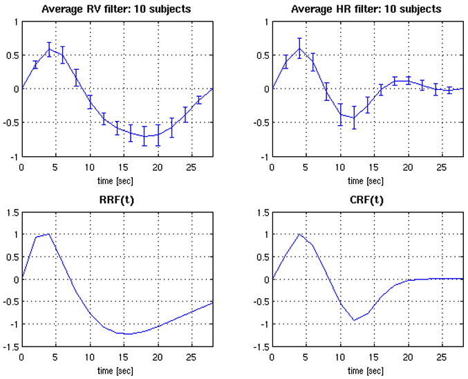
Deconvolved HR (A) and RV (B) filters from the RVHR model, averaged over 10 subjects. Error bars show the standard error. (C) RRF model from (Birn et al., 2008b). (D) Analytic function fitted to the average HR filter.

Figure 7.

Clustering of HR filters across voxels. The mean HR filter for each cluster is shown on the right (C), in decreasing order of cluster size (1=largest, 6=smallest). Color-coded maps showing the locations of each cluster for 2 subjects (A,B) are on the left.

Generalization of the average HR filter

To examine whether the average HR filter obtained from our subject population is generalizable, we applied it to a set of 3 subjects from a separate study who had each undergone one 8 min resting state scan. An analytic function (CRF(t), for “cardiac response function”) was fit to the curve as the sum of a Gamma and a Gaussian:

$$\mathit{CRF}(t)=0.6t^{2.7}{e}^{-t/1.6}-16\frac{1}{\sqrt{2\pi (9)}}\exp (-\frac{1}{2}\frac{{(t-12)}^2}{9})$$ (5)

(Figure 6D), and this function was used as the HR filter for all voxels. Two models were then evaluated on each of the 3 subjects’ resting state scans: (1) the RRF model, as described previously; and (2) the “RRF-CRF” model, in which the HR time series, convolved with CRF(t), was included as a covariate in the linear model. The RRF was used as the RV filter for each voxel since a separate scan was not available for deconvolving voxel-wise RV responses without bias, and because the RRF has been established both in the present study and in (Birn et al., 2008b) to well model the transfer function between RV and the BOLD signal. Maps of the variance explained by each model are shown for 2 subjects in Figure 8. Including HR convolved with CRF(t) contributed a significant amont of variance in all subjects’ resting state scans (Table 5), suggesting that CRF(t) is perhaps a generalizable transfer function between HR and the BOLD signal.

Figure 8.

Maps of the percent signal variance explained by the RRF (top line) and RRF-CRF (bottom line) models, for 3 subjects from a separate dataset.

Table 5. Variance explained by average HR model.

Variance explained by the RRF and RRF-CRF models on a separate set of 3 subjects (8 min resting state scan). The percentage of brain for which the indicated model explained a significant (p<0.0001; F-test) portion of signal variance is provided, along with the percent signal variance explained by the model (averaged across the set of significant voxels).

subj	RRF		RRF-CRF
	%brain	%var mean±sd	%brain	%var mean±sd
1	17.5	10.4±3.5	19.0	11.9±3.5
2	0.3	7.6±1.2	34.2	12.3±3.6
3	5.8	8.6±1.9	17.1	14.5±6.1
AVE	7.6	8.9±2.2	23.5	12.9±4.4

Consistency of the RV filter

Strong correlations were obtained between estimates of the RV filter resulting from the RVHR and RV models; that is, voxel-wise estimates of h_r and h͂_r were highly consistent despite the inclusion of HR in the RVHR model. The mean correlation across the set of voxels in which significant variance (p<0.001) was accounted for by both the RV and RVHR model was r=0.97 (SD=0.05); even when restricting the analysis to the set of voxels havng a significant (p<0.001) HR component in the RVHR model, strong correlations were maintained (r=0.93, SD=0.10). Similar generalization performance between the RV and RRF models reflects the fact that h_r and h͂_r were also well correlated with the RRF (r=0.74, SD=0.11 between h͂_r and the RRF).

Comparison of RV vs. RVT

The RV and RVT waveforms were correlated (mean r=0.61, SD=0.1 over the Rest2 scans of all 10 subjects). Minor differences were found in the shapes of the average filters when RVT was used instead of RV (Figure 9), though in comparing Figures 9A and 6A, we note that the error bars for each time point were slightly smaller when RV was used. Differences in the percentage variance explained when RVT was used instead of RV are shown in Table 6. While differences were again minor, there was a trend towared greater average variance explained when RV was used.

Figure 9.

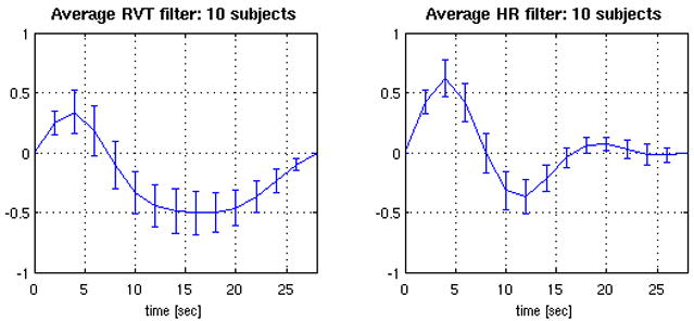
Deconvolved HR and RVT filters from the RVHR model, when RVT was used instead of RV. Curves depict the average (±SE) over 10 subjects.

Table 6. Comparison of RVT vs. RV.

A. Average percent variance explained by the various models. The first line (RV) is identical to the final row of Table 3, and the second line (RVT) indicates the corresponding values when RVT is used instead of RV.

B. Model comparison. The first line (RV) is identical to the final row of Table 4, and the second line (RVT) indicates the corresponding values when RVT is used instead of RV.

	RRF		RV		RVHR		RVHR: RV	RVHR: HR
	%brain	%var mean±sd	%brain	%var mean±sd	%brain	%var mean±sd	%var mean±sd	%var mean±sd
RV	24.8	11.0±3.8	28.3	11.7±4.3	45.3	15.8±6.3	7.4±5.6	8.2±6.1
RVT	18.0	10.0±3.1	22.3	10.6±3.6	40.2	14.7±5.8	6.0±4.6	8.6±5.7

	Model
	RVHR>RV (%)	RVHR>RRF (%)	RV>RRF (%)
RV	27.5	33.1	1.2
RVT	25.4	31.3	0.6

Impact of RETROICOR

Figure 10 reveals how the extent of DMN connectivity changed after correction using RETROICOR, RVHR, and both RETROICOR and RVHR. It is apparent that (1) applying RETROICOR alone influenced the outcome of DMN connectivity slightly, (2) connectivity changes due to RVHR were much greater than those induced by applying RETROICOR (p<0.05), and (3) the extent (volume) of change due to applying RETROICOR before RVHR was similar to that of applying RVHR alone (p>0.05; n.s.). Figure 11 illustrates the connectivity maps for one subject.

Figure 10.

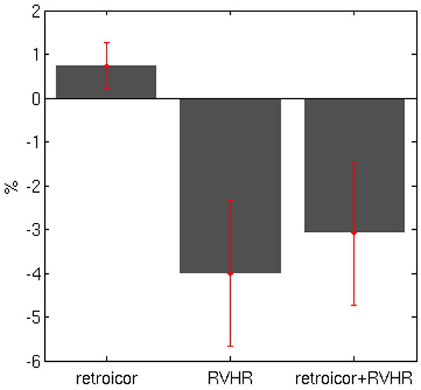
Default-mode network changes due to correction with RETROICOR, RVHR, and both RETROICOR and RVHR. Bar height indicates the mean percent change in the extent of voxels having significant (p<0.05) DMN connectivity following the indicated corrections. The sign of each bar reveals the direction of change (negative = smaller connectivity extent; positive = larger connectivity extent).

Figure 11.

Comparison of default-mode network maps with (A) no correction, (B) correction using RETROICOR, (C) correction using the RVHR model, (D) correction using both RETROICOR and RVHR.

Discussion

The present study demonstrates that a linear systems model having both RV and HR inputs can account for substantial fluctuations in the resting state BOLD signal. The RVHR model explained a significantly greater fraction of signal variance beyond the RV model, and over a spatial extent encompassing widespread regions of gray matter. A HR hemodynamic response function (CRF(t)) is proposed, and is shown to adequately characterize the mapping between HR and the BOLD signal for our subject population. Furthermore, results verify that the RV response function (RRF) introduced by Birn et al. represents well the mapping between RV and the BOLD signal, even when simultaneously accounting for HR. Moreover, removing HR and RV components from the BOLD signal using our RVHR model can induce significant changes (region-specific reductions as well as increases) in resting state network connectivity.

The RV and HR filters were deconvolved using Gaussian process priors. This yields smooth (and thus physiologically plausible) response functions, and so presents a suitable approach to the problem of deconvolving physiological contributions to the BOLD signal. This method avoids the noise amplification problem of unconstrained deconvolution which has led others (e.g. (Birn et al., 2008b)) to use less straightforward approaches. In addition, the framework for simultaneous deconvolution employed in the current study can be directly extended to incorporate additional physiological or neural inputs that may be of future interest.

In agreement with Shmueli et al., HR was found to contribute significant additional variance beyond RV in gray matter as well as in regions expected to be more susceptible to cardiac pulsatility, such as CSF and major vessels (Shmueli et al., 2007). Importantly, as illustrated in Figure 3, regions in which the HR component had a significant effect were often disjoint from regions in which the effects of RV (and RRF) were significant, indicating differential contributions of HR and RV effects over space. Variability was observed across subjects with respect to both magnitude and spatial location of significant HR effects, and a group analysis did not reveal any particular anatomical regions that were highly significant for HR. While the mechanism through which HR could modulate the BOLD signal is not well-understood, gray matter correlations with HR could be due in part to neuronal activity linked with changes in levels of arousal.

Deconvolution of the HR response revealed that the majority of responsive voxels exhibited a peak at around 4 sec and an undershoot of approximately equal magnitude at around 12 sec. These features were remarkably consistent across subjects and anatomical regions, and generalized well to a separate population of 3 subjects. The use of this proposed average HR filter (CRF), in conjunction with the average RV filter (RRF) proposed by Birn et al., may thus present an alternative to voxel-wise deconvolution for reducing the influence of HR and RV in the BOLD signal, obviating the need for an additional scan.

However, if obtaining voxel-wise RV and HR filters is desired, appending a 12 min scan in order to implement the RVHR model on other functional scans would be expensive and time-consuming; thus, it is of interest to know whether a shorter scan will suffice. We evaluated the stability of deconvolved HR responses for one subject using only the first 4 min and 8 min of the 12 min Rest1 scan, for voxels in which the RVHR model was significant (p<0.001). As shown in Figure 12, 8 min of data sufficed to yield responses that were highly similar to those from 12 min.

Figure 12.

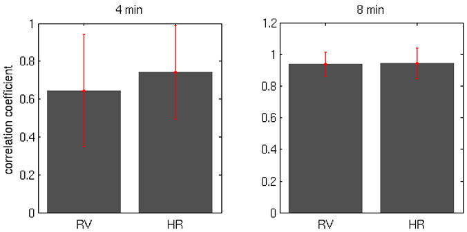
Average correlation (±SD) between voxel-wise RV and HR filters from 4 min versus 12 min of data (left), and 8 min versus 12 min of data (right).

Voxel-wise estimates of the RV impulse response were only slightly more effective (and for 3 subjects, less effective) in accounting for variance in the second resting state scan compared to using the RRF for all voxels. In addition, the amount of spatial ovelap was substantial, consistent with the fact that our deconvolved RV impulse responses were similar in character to the RRF – even when simultaneously accounting for HR, and despite the fact that RV (rather than RVT) was used as the respiration input function. This finding suggests that the RRF is indeed an effective a priori RV response function, which is further demonstrated by our result showing that the RRF correction impacts maps of the DMN, a finding that extends Birn’s results from correction based on cross-correlation (Birn et al., 2006) to use of the RRF (Birn et al., 2008b). Furthermore, convolving RV with the RRF was shown to provide a better fit to resting state data than a simple cross-correlation; this is somewhat different from the results of Birn et al., 2008b, who had found that the RRF accurately modeled BOLD signal changes to cued-breathing paradigms but did not fit resting state data more effectively than cross-correlation

We chose to deconvolve RV and HR simultaneously, rather than HR alone, because (a) RV is known to account for significant portion of the BOLD signal and it is therefore critical to model it, and (b) possible interactions between RV and HR may result in different filters than if either were estimated alone. Respiratory and cardiac processes are intimately related, and both govern cerebral blood flow and oxygenation and hence BOLD signal changes. Yet, we observed strong correlations between RV filters deconvolved using the RVHR and RV models, even for the set of voxels demonstrating a significant HR component. That modeling HR had a negligible impact on the deconvolved RV filters suggests a degree of independence between the way in which RV and HR may propagate into the BOLD signal.

The RVHR corrections altered DMN maps beyond corrections using RV alone, though both models acted primarily to diminish connectivity with the PCC. It is not possible to quantify the goodness of network changes, as there is no ground truth for which regions ought to comprise the network, and it is not clear to what extent previous characterizations of the DMN reflect physiological, rather than neural, connectivity. However, “canonical” nodes of the DMN are believed to be those showing task-correlated deactivation (Greicius et al., 2003; Raichle et al., 2001) and reduction of connectivity outside of these regions is viewed as desirable. In our study, brain regions were not affected uniformly by RV or RVHR correction; with reference to Figure 5, connectivity of canonical nodes such as the medial prefrontal cortex and anterior cingulate cortex was preserved or increased, whereas regions outside of the network tended to decrease. Hence, modeling both RV and HR can potentially reduce the number of false positives in functional connectivity analysis.

Importantly, Figures 4 and 5 also reveal that the spatial extent of RV and HR fluctuations overlaps substantially with at least one of the resting state networks, the DMN. This suggests that data-driven approaches such as ICA will not be able to fully distinguish between neural sources of connectivity and those due to physiological processes such as RV and HR (Birn et al., 2008a), and therefore, that preprocessing resting state data with the RVHR correction would be useful, especially when quantification of network extent is desired.

It is fairly common in the literature to apply a “global signal” correction, in which a whole-brain average signal is regressed out of each voxel time series prior to analyzing functional connectivity (e.g. (Di Martino et al., 2008; Fair et al., 2008; Fox et al., 2005)). While having the desired effect of making networks more focal, the global signal represents a mixture of physiological, neural, and movement-related sources, and regressing it out will unfortunately remove common signal as well as common noise. Large networks whose constituent regions exhibit large BOLD signal changes, such as the DMN, may contribute substantially to the global average. On the other hand, approaches that model and correct for physiological noise based on external measures, such as the respiration and cardiac monitoring, can reduce potential noise in an unbiased way.

Because we aim to model and remove physiological noise due to cardiac and respiratory processes beyond those simply time-locked to the cardiac and respiratory cycles, correction was initially intended to be applied post-RETROICOR. We observed that quantitative changes in the spatial extent of variance explained (and DMN connectivity) when applying the RVHR model with and without RETROICOR were small; however, such a quantification does not characterize any possible spatial dispartity or ’goodness’ of the change, nor does it reveal any overlap between the effects of both corrections. It is interesting that although the signal components treated by RETROICOR and RVHR are in a sense distinct (though having a common physiological origin), the effects from correction using the 2 methods can be similar, as seen in the DMN for the subject in Figure 11. RETROICOR and RVHR produced comparable changes in the DMN. In this subject, as well as several others, applying RETROICOR with RVHR produced greater changes in DMN connectivity (again, mainly reductions) than applying either in isolation.

Our measure of RV consisted of the sliding-window standard deviation of the respiratory belt waveform, and thus relates primarily to changes in inspiration depth over time. While simpler to compute than RVT (no peak detection in the respiration waveform is required), the use of a fixed-length sliding window rather than breath-to-breath intervals is more difficult to interpret due to its complex dependence on the depth, frequency, and phase of respiratory cycle within each window, especially when the breathing rate is slow relative to the window length. However, our RV measure tended to correlate with RVT) in our set of subjects, and the average RV transfer function agreed with the RVT transfer function (RRF) of (Birn et al., 2008b). In addition, a re-analysis of our data using RVT instead of RV yielded minor differences in the results. While it is encouraging that two slightly different quantifications of respiratory variation from a pneumatic belt waveform can explain similar variance in the BOLD signal, the optimal way to relate measurements of chest expansion during breathing to parameters that more directly mediate BOLD signal change, such as end-tidal CO2, requires further investigation.

In summary, a canonical HR response function is proposed that, in conjunction with the RRF and with or without RETROICOR, can result in significant and widespread reductions of variance in resting BOLD contrast timeseries when applied in a linear model. The relative contribution of HR and RV to BOLD fluctuations was not uniform across subjects; sometimes HR was more prominent than RV, and in other cases less so. In general, applying RVHR corrections resulted in diminished spatial extent of the resting state DMN to a greater degree than with RV corrections alone. This suggests that caution should be exercised when employing quantitative analyses of resting state networks, without accounting for physiological noise sources from both cardiac and respiratory functions.

Figure 1.

Example of physiological time courses for 1 subject, showing (A) respiration belt measurements, (B) the calculated RV, (C) cardiac cycle with triggers, and (D) the calculated HR. Note that (A,B) are displayed on a different time scale than (C,D).

Appendix A

As described in the text, the model (Eq. 1) can be written compactly as y = Xh+ε, and a Gaussian process prior is placed on h: h ~ N(0,K). In the Bayesian framework, we would like to find h to maximize p(h | y), which is known as the maximum a posteriori (MAP) solution. Following Bayes’ rule, the posterior distribution of over h is given by

$$p(h|y)=\frac{p(y|h)p(h)}{p(y)},$$ (6)

where $p(y|h)=N(Xh,{\sigma }_{\epsilon }^{2}I)$ (I is the identity matrix) and the marginal likelihood p(y) is independent of h. Including only the terms that are dependent on h (i.e. the numerator of Eq. 6), we obtain

$$p(h|y)\propto \exp -\frac{1}{2{\sigma }_{\epsilon }^2}{(y-Xh)}^T(y-Xh)\exp -\frac{1}{2}{h}^T{K}^{-1}h.$$ (7)

Since maximing p(h | y) is equivalent to minimizing -log p(h | y), the problem reduces to minimizing

$$-\log p(h|y)\propto \frac{1}{{\sigma }_{\epsilon }^2}{(y-Xh)}^T(y-Xh)+h^T{K}^{-1}h.$$ (8)

Setting the gradient with respect to h of Eq. 8 to 0 and solving for h yields

$$h_{\mathrm{MAP}}={(X^{T}X+{\sigma }_{\epsilon }^2{K}^{-1})}^{-1}{X}^{T}y,$$ (9)

which is the result provided in Eq. 2.

Appendix B

When estimating h_r and h_h, we wish to enforce the sensible constraint that both filters begin and end at 0. Optimization theory offers a method to incorporate this constraint into the MAP estimate of Eq. 9, which is based on the KKT conditions and described in many optimization texts (see, e.g., (Boyd and Vandenberghe, 2004)). A brief overview of our treatment follows.

To implement the constraint that h_r and h_h (which are of length n_r and n_h, respectively) each begin and end at 0, we solve the quadratic optimization problem

$$\begin{array}{ll}\underset{h}{\mathrm{minimize}}& \frac{1}{{\sigma }_{\epsilon }^2}{(y-\mathit{Xh})}^T(y-\mathit{Xh})+h^T\mathit{Rh}\\ \mathrm{subject\; to}& \mathit{Sh}=0,\end{array}$$ (10)

where S is a 4x(n_r+n_h) selector matrix consisting of ones at the (1,1), (2, n_r), (3, n_r +1) and (4, n_r +n_h) entries and zeros elsewhere, and R = K^-1. The objective function in Eq. (10) results from wishing to maximize p (h | y) (Eq. 8). The KKT conditions specify that the optimal solution satisfies

$${\mathit{Sh}}^{\ast }=0$$ (11)

and

$$2(\frac{X^{T}X}{{\sigma }_{\epsilon }^2}+R)h^{\ast }-\frac{2}{{\sigma }_{\epsilon }^2}{X}^{T}y+S^T{\upsilon }^{\ast }=0,$$ (12)

where h* and υ* are the optimal primal and dual variables. The condition (12) results from the fact that the gradient of the Lagrangian must vanish at h* and υ*. Equations (11) and (12) define the linear system

$$\begin{array}{ccccc}2(\frac{X^{T}X}{{{\displaystyle \sigma }}_{\epsilon }^2}+R)& S^T& h^{\ast }& =& \frac{2}{{{\displaystyle \sigma }}_{\epsilon }^2}{X}^{T}y\\ S& 0& {\upsilon }^{\ast }& 0\end{array},$$ (13)

which can be solved efficiently for both h* and υ*.

References

- Bandettini PA, Wong EC, Hinks RS, Tikofsky RS, Hyde JS. Time course EPI of human brain function during task activation. Magn Reson Med. 1992;25:390–397. doi: 10.1002/mrm.1910250220. [DOI] [PubMed] [Google Scholar]
- Binder JR, Frost JA, Hammeke TA, Bellgowan PS, Rao SM, Cox RW. Conceptual processing during the conscious resting state. A functional MRI study. J Cogn Neurosci. 1999;11:80–95. doi: 10.1162/089892999563265. [DOI] [PubMed] [Google Scholar]
- Birn RM, Diamond JB, Smith MA, Bandettini PA. Separating respiratory-variation-related fluctuations from neuronal-activity-related fluctuations in fMRI. Neuroimage. 2006;31:1536–1548. doi: 10.1016/j.neuroimage.2006.02.048. [DOI] [PubMed] [Google Scholar]
- Birn RM, Murphy K, Bandettini PA. The effect of respiration variations on independent component analysis results of resting state functional connectivity. Hum Brain Mapp. 2008a doi: 10.1002/hbm.20577. [DOI] [PMC free article] [PubMed] [Google Scholar]
- Birn RM, Smith MA, Jones TB, Bandettini PA. The respiration response function: The temporal dynamics of fMRI signal fluctuations related to changes in respiration. Neuroimage. 2008b;40:644–654. doi: 10.1016/j.neuroimage.2007.11.059. [DOI] [PMC free article] [PubMed] [Google Scholar]
- Biswal B, Yetkin FZ, Haughton VM, Hyde JS. Functional connectivity in the motor cortex of resting human brain using echo-planar MRI. Magn Reson Med. 1995;34:537–541. doi: 10.1002/mrm.1910340409. [DOI] [PubMed] [Google Scholar]
- Boyd SP, Vandenberghe L. Convex Optimization. Cambridge University Press; Cambridge, U.K: 2004. pp. 243–244. [Google Scholar]
- Casanova R, Ryali S, Serences J, Yang L, Kraft R, Laurienti PJ, Maldjian JA. The impact of temporal regularization on estimates of the BOLD hemodynamic response function: a comparative analysis. Neuroimage. 2008;40:1606–1618. doi: 10.1016/j.neuroimage.2008.01.011. [DOI] [PMC free article] [PubMed] [Google Scholar]
- Clare Kelly AM, Uddin LQ, Biswal BB, Castellanos FX, Milham MP. Competition between functional brain networks mediates behavioral variability. Neuroimage. 2008;39:527–537. doi: 10.1016/j.neuroimage.2007.08.008. [DOI] [PubMed] [Google Scholar]
- Cordes D, Haughton VM, Arfanakis K, Carew JD, Turski PA, Moritz CH, Quigley MA, Meyerand ME. Frequencies contributing to functional connectivity in the cerebral cortex in “resting-state” data. AJNR Am J Neuroradiol. 2001;22:1326–1333. [PMC free article] [PubMed] [Google Scholar]
- Corfield DR, Murphy K, Josephs O, Adams L, Turner R. Does hypercapnia-induced cerebral vasodilation modulate the hemodynamic response to neural activation? Neuroimage. 2001;13:1207–1211. doi: 10.1006/nimg.2001.0760. [DOI] [PubMed] [Google Scholar]
- Dagli MS, Ingeholm JE, Haxby JV. Localization of cardiac-induced signal change in fMRI. Neuroimage. 1999;9:407–415. doi: 10.1006/nimg.1998.0424. [DOI] [PubMed] [Google Scholar]
- Damoiseaux JS, Beckmann CF, Arigita EJ, Barkhof F, Scheltens P, Stam CJ, Smith SM, Rombouts SA. Reduced resting-state brain activity in the “default network” in normal aging. Cereb Cortex. 2007 doi: 10.1093/cercor/bhm207. [DOI] [PubMed] [Google Scholar]
- Daselaar SM, Prince SE, Cabeza R. When less means more: deactivations during encoding that predict subsequent memory. Neuroimage. 2004;23:921–927. doi: 10.1016/j.neuroimage.2004.07.031. [DOI] [PubMed] [Google Scholar]
- Deckers RH, van Gelderen P, Ries M, Barret O, Duyn JH, Ikonomidou VN, Fukunaga M, Glover GH, de Zwart JA. An adaptive filter for suppression of cardiac and respiratory noise in MRI time series data. Neuroimage. 2006;33:1072–1081. doi: 10.1016/j.neuroimage.2006.08.006. [DOI] [PMC free article] [PubMed] [Google Scholar]
- Di Martino A, Scheres A, Margulies DS, Kelly AM, Uddin LQ, Shehzad Z, Biswal B, Walters JR, Castellanos FX, Milham MP. Functional Connectivity of Human Striatum: A Resting State fMRI Study. Cereb Cortex. 2008 doi: 10.1093/cercor/bhn041. [DOI] [PubMed] [Google Scholar]
- Dowdy S, Wearden S. Statistics for Research. Wiley Interscience; New York, N.Y: 1991. p. 267. [Google Scholar]
- Fair DA, Cohen AL, Dosenbach NU, Church JA, Miezin FM, Barch DM, Raichle ME, Petersen SE, Schlaggar BL. The maturing architecture of the brain’s default network. Proc Natl Acad Sci U S A. 2008;105:4028–4032. doi: 10.1073/pnas.0800376105. [DOI] [PMC free article] [PubMed] [Google Scholar]
- Fox MD, Snyder AZ, Vincent JL, Corbetta M, Van Essen DC, Raichle ME. The human brain is intrinsically organized into dynamic, anticorrelated functional networks. Proc Natl Acad Sci U S A. 2005;102:9673–9678. doi: 10.1073/pnas.0504136102. [DOI] [PMC free article] [PubMed] [Google Scholar]
- Freire L, Mangin JF. Motion correction algorithms may create spurious brain activations in the absence of subject motion. Neuroimage. 2001;14:709–722. doi: 10.1006/nimg.2001.0869. [DOI] [PubMed] [Google Scholar]
- Friston KJ, Williams S, Howard R, Frackowiak RS, Turner R. Movement-related effects in fMRI time-series. Magn Reson Med. 1996;35:346–355. doi: 10.1002/mrm.1910350312. [DOI] [PubMed] [Google Scholar]
- Garrity AG, Pearlson GD, McKiernan K, Lloyd D, Kiehl KA, Calhoun VD. Aberrant “default mode” functional connectivity in schizophrenia. Am J Psychiatry. 2007;164:450–457. doi: 10.1176/ajp.2007.164.3.450. [DOI] [PubMed] [Google Scholar]
- Glover GH, Lai S. Self-navigated spiral fMRI: interleaved versus single-shot. Magnetic Resonance in Medicine. 1998;39:361–368. doi: 10.1002/mrm.1910390305. [DOI] [PubMed] [Google Scholar]
- Glover GH, Law CS. Spiral-in/out BOLD fMRI for increased SNR and reduced susceptibility artifacts. Magn Reson Med. 2001;46:515–522. doi: 10.1002/mrm.1222. [DOI] [PubMed] [Google Scholar]
- Glover GH, Li TQ, Ress D. Image-based method for retrospective correction of physiological motion effects in fMRI: RETROICOR. Magn Reson Med. 2000;44:162–167. doi: 10.1002/1522-2594(200007)44:1<162::aid-mrm23>3.0.co;2-e. [DOI] [PubMed] [Google Scholar]
- Goutte C, Nielsen FA, Hansen LK. Modeling the haemodynamic response in fMRI using smooth FIR filters. IEEE Trans Med Imaging. 2000;19:1188–1201. doi: 10.1109/42.897811. [DOI] [PubMed] [Google Scholar]
- Greicius MD, Flores BH, Menon V, Glover GH, Solvason HB, Kenna H, Reiss AL, Schatzberg AF. Resting-State Functional Connectivity in Major Depression: Abnormally Increased Contributions from Subgenual Cingulate Cortex and Thalamus. Biol Psychiatry. 2007 doi: 10.1016/j.biopsych.2006.09.020. [DOI] [PMC free article] [PubMed] [Google Scholar]
- Greicius MD, Krasnow B, Reiss AL, Menon V. Functional connectivity in the resting brain: a network analysis of the default mode hypothesis. Proc Natl Acad Sci U S A. 2003;100:253–258. doi: 10.1073/pnas.0135058100. [DOI] [PMC free article] [PubMed] [Google Scholar]
- Greicius MD, Menon V. Default-mode activity during a passive sensory task: uncoupled from deactivation but impacting activation. J Cogn Neurosci. 2004;16:1484–1492. doi: 10.1162/0898929042568532. [DOI] [PubMed] [Google Scholar]
- Greicius MD, Srivastava G, Reiss AL, Menon V. Default-mode network activity distinguishes Alzheimer’s disease from healthy aging: evidence from functional MRI. Proc Natl Acad Sci U S A. 2004;101:4637–4642. doi: 10.1073/pnas.0308627101. [DOI] [PMC free article] [PubMed] [Google Scholar]
- Gusnard DA, Raichle ME, Raichle ME. Searching for a baseline: functional imaging and the resting human brain. Nat Rev Neurosci. 2001;2:685–694. doi: 10.1038/35094500. [DOI] [PubMed] [Google Scholar]
- Hampson M, Driesen NR, Skudlarski P, Gore JC, Constable RT. Brain connectivity related to working memory performance. J Neurosci. 2006;26:13338–13343. doi: 10.1523/JNEUROSCI.3408-06.2006. [DOI] [PMC free article] [PubMed] [Google Scholar]
- Hu X, Le TH, Parrish T, Erhard P. Retrospective estimation and correction of physiological fluctuation in functional MRI. Magn Reson Med. 1995;34:201–212. doi: 10.1002/mrm.1910340211. [DOI] [PubMed] [Google Scholar]
- Kastrup A, Kruger G, Glover GH, Moseley ME. Assessment of cerebral oxidative metabolism with breath holding and fMRI. Magn Reson Med. 1999a;42:608–611. doi: 10.1002/(sici)1522-2594(199909)42:3<608::aid-mrm26>3.0.co;2-i. [DOI] [PubMed] [Google Scholar]
- Kastrup A, Kruger G, Glover GH, Neumann-Haefelin T, Moseley ME. Regional variability of cerebral blood oxygenation response to hypercapnia. Neuroimage. 1999b;10:675–681. doi: 10.1006/nimg.1999.0505. [DOI] [PubMed] [Google Scholar]
- Kastrup A, Li TQ, Glover GH, Moseley ME. Cerebral blood flow-related signal changes during breath-holding. AJNR Am J Neuroradiol. 1999c;20:1233–1238. [PMC free article] [PubMed] [Google Scholar]
- Kastrup A, Li TQ, Takahashi A, Glover GH, Moseley ME. Functional magnetic resonance imaging of regional cerebral blood oxygenation changes during breath holding. Stroke. 1998;29:2641–2645. doi: 10.1161/01.str.29.12.2641. [DOI] [PubMed] [Google Scholar]
- Kim DH, Adalsteinsson E, Glover GH, Spielman DM. Regularized higher-order in vivo shimming. Magn Reson Med. 2002;48:715–722. doi: 10.1002/mrm.10267. [DOI] [PubMed] [Google Scholar]
- Kwong KK, Belliveau JW, Chesler DA, Goldberg IE, Weisskoff RM, Poncelet BP, Kennedy DN, Hoppel BE, Cohen MS, Turner R. Dynamic magnetic resonance imaging of human brain activity during primary sensory stimulation. Proc Natl Acad Sci U S A. 1992;89:5675–5679. doi: 10.1073/pnas.89.12.5675. [DOI] [PMC free article] [PubMed] [Google Scholar]
- Liu HL, Huang JC, Wu CT, Hsu YY. Detectability of blood oxygenation level-dependent signal changes during short breath hold duration. Magn Reson Imaging. 2002;20:643–648. doi: 10.1016/s0730-725x(02)00595-7. [DOI] [PubMed] [Google Scholar]
- Marrelec G, Benali H, Ciuciu P, Pelegrini-Issac M, Poline JB. Robust Bayesian estimation of the hemodynamic response function in event-related BOLD fMRI using basic physiological information. Hum Brain Mapp. 2003a;19:1–17. doi: 10.1002/hbm.10100. [DOI] [PMC free article] [PubMed] [Google Scholar]
- Marrelec G, Ciuciu P, Pelegrini-Issac M, Benali H. Estimation of the Hemodynamic Response Function in event-related functional MRI: directed acyclic graphs for a general Bayesian inference framework. Inf Process Med Imaging. 2003b;18:635–646. doi: 10.1007/978-3-540-45087-0_53. [DOI] [PubMed] [Google Scholar]
- Marrelec G, Ciuciu P, Pelegrini-Issac M, Benali H. Estimation of the hemodynamic response in event-related functional MRI: Bayesian networks as a framework for efficient Bayesian modeling and inference. IEEE Trans Med Imaging. 2004;23:959–967. doi: 10.1109/TMI.2004.831221. [DOI] [PubMed] [Google Scholar]
- Mazoyer B, Zago L, Mellet E, Bricogne S, Etard O, Houde O, Crivello F, Joliot M, Petit L, Tzourio-Mazoyer N. Cortical networks for working memory and executive functions sustain the conscious resting state in man. Brain Res Bull. 2001;54:287–298. doi: 10.1016/s0361-9230(00)00437-8. [DOI] [PubMed] [Google Scholar]
- McKiernan KA, Kaufman JN, Kucera-Thompson J, Binder JR. A parametric manipulation of factors affecting task-induced deactivation in functional neuroimaging. J Cogn Neurosci. 2003;15:394–408. doi: 10.1162/089892903321593117. [DOI] [PubMed] [Google Scholar]
- Nakada K, Yoshida D, Fukumoto M, Yoshida S. Chronological analysis of physiological T2* signal change in the cerebrum during breath holding. J Magn Reson Imaging. 2001;13:344–351. doi: 10.1002/jmri.1049. [DOI] [PubMed] [Google Scholar]
- Ogawa S, Tank DW, Menon R, Ellermann JM, Kim SG, Merkle H, Ugurbil K. Intrinsic signal changes accompanying sensory stimulation: functional brain mapping with magnetic resonance imaging. Proc Natl Acad Sci U S A. 1992;89:5951–5955. doi: 10.1073/pnas.89.13.5951. [DOI] [PMC free article] [PubMed] [Google Scholar]
- Pfeuffer J, Van de Moortele PF, Ugurbil K, Hu X, Glover GH. Correction of physiologically induced global off-resonance effects in dynamic echo-planar and spiral functional imaging. Magn Reson Med. 2002;47:344–353. doi: 10.1002/mrm.10065. [DOI] [PubMed] [Google Scholar]
- Raichle ME, MacLeod AM, Snyder AZ, Powers WJ, Gusnard DA, Shulman GL. A default mode of brain function. Proc Natl Acad Sci U S A. 2001;98:676–682. doi: 10.1073/pnas.98.2.676. [DOI] [PMC free article] [PubMed] [Google Scholar]
- Rasmussen CE. Conjugate Gradient Minimizer - ’minimize.m’ function in MATLAB 2006 [Google Scholar]
- Rasmussen CE, Williams CKI. Gaussian Processes for Machine Learning. The MIT Press; Cambridge, MA: 2006. [Google Scholar]
- Shmueli K, van Gelderen P, de Zwart JA, Horovitz SG, Fukunaga M, Jansma JM, Duyn JH. Low-frequency fluctuations in the cardiac rate as a source of variance in the resting-state fMRI BOLD signal. Neuroimage. 2007;38:306–320. doi: 10.1016/j.neuroimage.2007.07.037. [DOI] [PMC free article] [PubMed] [Google Scholar]
- Shulman GL, Corbetta M, Buckner RL, Raichle ME, Fiez JA, Miezin FM, Petersen SE. Top-down modulation of early sensory cortex. Cereb Cortex. 1997;7:193–206. doi: 10.1093/cercor/7.3.193. [DOI] [PubMed] [Google Scholar]
- Thomason ME, Chang CE, Glover GH, Gabrieli JD, Greicius MD, Gotlib IH. Default-Mode Function and Task-Induced Deactivation Have Overlapping Brain Substrates in Children. Neuroimage. 2008 doi: 10.1016/j.neuroimage.2008.03.029. [DOI] [PMC free article] [PubMed] [Google Scholar]
- Thomason ME, Glover GH. Controlled inspiration depth reduces variance in breath-holding-induced BOLD signal. Neuroimage. 2008;39:206–214. doi: 10.1016/j.neuroimage.2007.08.014. [DOI] [PMC free article] [PubMed] [Google Scholar]
- Uddin LQ, Kelly AM, Biswal BB, Margulies DS, Shehzad Z, Shaw D, Ghaffari M, Rotrosen J, Adler LA, Castellanos FX, Milham MP. Network homogeneity reveals decreased integrity of default-mode network in ADHD. J Neurosci Methods. 2008;169:249–254. doi: 10.1016/j.jneumeth.2007.11.031. [DOI] [PubMed] [Google Scholar]
- Wise RG, Ide K, Poulin MJ, Tracey I. Resting fluctuations in arterial carbon dioxide induce significant low frequency variations in BOLD signal. Neuroimage. 2004;21:1652–1664. doi: 10.1016/j.neuroimage.2003.11.025. [DOI] [PubMed] [Google Scholar]