A feature-based approach to modeling protein–protein interaction hot spots

Abstract

Identifying features that effectively represent the energetic contribution of an individual interface residue to the interactions between proteins remains problematic. Here, we present several new features and show that they are more effective than conventional features. By combining the proposed features with conventional features, we develop a predictive model for interaction hot spots. Initially, 54 multifaceted features, composed of different levels of information including structure, sequence and molecular interaction information, are quantified. Then, to identify the best subset of features for predicting hot spots, feature selection is performed using a decision tree. Based on the selected features, a predictive model for hot spots is created using support vector machine (SVM) and tested on an independent test set. Our model shows better overall predictive accuracy than previous methods such as the alanine scanning methods Robetta and FOLDEF, and the knowledge-based method KFC. Subsequent analysis yields several findings about hot spots. As expected, hot spots have a larger relative surface area burial and are more hydrophobic than other residues. Unexpectedly, however, residue conservation displays a rather complicated tendency depending on the types of protein complexes, indicating that this feature is not good for identifying hot spots. Of the selected features, the weighted atomic packing density, relative surface area burial and weighted hydrophobicity are the top 3, with the weighted atomic packing density proving to be the most effective feature for predicting hot spots. Notably, we find that hot spots are closely related to π–related interactions, especially π · · · π interactions.

INTRODUCTION

For cellular function, proteins interact with other molecules, with the nature of these interactions depending on the physiological conditions. Several techniques have been adopted to obtain a global view of the physical interactions between proteins (e.g. yeast-two-hybrid and tandem affinity purifications) (1,2). Systematic analyses (3–15) of a variety of protein–protein interaction interfaces have shown that there are no general rules that clearly describe such interfaces. Studies of these interfaces have produced variable results, partly because they have examined different types of proteins; hence, when comparing findings for different proteins, it is important to consider the types of proteins (16,17).

The question of which residues are energetically more important in protein–protein interaction interfaces is a long-standing issue whose resolution would have significant implications for practical applications, such as rational drug design and protein engineering. Biophysical characterization of protein–protein interaction interfaces has been achieved through alanine-scanning mutagenesis (18–20). Despite the large sizes of these binding interfaces, individual single side chains can contribute a large fraction of the binding free energy (21,22). A database of alanine mutations is now accessible through the Internet for systematic analysis (23). The ‘O-ring model’ has been suggested to explain the relationship between the change in free energy associated with binding, ΔΔG, and solvent accessibility in the complexes (24).

To complement the low-throughput of wet-experiments and to enhance the understanding of protein stability, computational prediction methods have been proposed (25–28). Most such studies have used thermodynamic simulation to estimate the free energy of association. Although these methods include energy terms, which are important for protein stability, there is still a large discrepancy between predicted values and experimentally measured free energy changes. Recently, a knowledge-based model was introduced to predict binding ‘hot spots’ (29,30), but the prediction accuracy was relatively low. In addition, the biological meaning of each feature has not been investigated.

Efforts have been made to identify correlations between binding hot spots and protein structure and sequence information (31–34). These studies disclosed that structurally conserved residues are strongly correlated with experimentally identified hot spots and that hot spots are distributed within the interface rather than compactly clustered. Moreover, the identification of similar residue hot spots in various protein families may suggest that affinity and specificity are not necessarily coupled.

Although, since Bogan's; initial study (24), several studies have examined hot spots, systematic analysis of the structural features is limited to the solvent accessibility and surface area burial between the unbound and bound states (ΔASA). In addition, only qualitative analyses have been performed, and statistical analysis has not been applied. The qualitative nature of the analyses performed to date mainly derives from the difficulty of identifying features that distinguish hot spots from other residues in interaction interfaces.

Here, we apply a feature-based approach to modeling protein–protein interaction hot spots. We create several new features quantified by a new measure, and show that the proposed features are more effective than the conventional features. By combining our new features with the conventional features, we develop a predictive model for interaction hot spots. Initially, 54 multifaceted features, composed of different levels of information, including structure, sequence and molecular interaction data, are quantified. Then, feature selection is performed using a decision tree to identify the best subset of features to predict hot spots. For this process, 265 alanine-mutated interface residues in 17 complexes are collected and categorized either as hot spots or energetically unimportant residues, based on a definition of hot spots. We used two definitions for hot spots, ΔΔG ≥ 1.0 kcal/mol or ΔΔG ≥ 2.0 kcal/mol. Using ΔΔG ≥ 1.0 kcal/mol to define hot spots, the interface residues are divided into 119 hot spots and 146 energetically unimportant residues (i.e. the T1 training set, see Materials and methods section). When ΔΔG ≥ 2.0 kcal/mol is used for hot spots, the interface residues are grouped into 65 hot spots and 200 energetically unimportant residues (i.e. the T2 training set, see Materials and methods section). With these two training sets, predictive models for hot spots are created with support vector machine (SVM), and tested with 10-fold cross-validation. Apart from these data, an independent test set, composed of 127 alanine-mutated interface residues in 18 complexes, is also constructed from the Binding Interface Database (BID; http://tsailab.org/BID/) (35) to further validate our predictive models. Comparison of our models with other methods such as alanine scanning methods [Robetta (27), FOLDEF (28)] and knowledge-based methods (K-FADE, K-CON) (29,30) disclosed that our SVM models give better predictive performance than other methods.

Feature selection can preserve the original semantics of the input features, allowing us to directly interpret the biological and statistical meanings of the features selected to train the models. Of the selected features, the top 3 based on discriminating power are the weighted atomic packing density, relative surface area burial and weighted hydrophobicity, which are located in the upper levels of the decision tree. All of these features are newly proposed here. Especially, the weighted atomic packing density, which reflects the contribution of an individual interface residue to the whole interface area (36), proves to be the most effective feature to discriminate hot spots from the other residues in an interface. Other structural features, such as the relative surface burial, solvent accessibility and surface area burial (ΔASA), are also investigated. Evolutionary information (conservation), chemical properties (weighted hydrophobicity) and molecular interaction information are also exhaustively analyzed.

MATERIALS AND METHODS

Our research flow consists of six steps: ‘Data collection’, ‘Feature generation’, ‘Data representation’, ‘Feature selection’, ‘Model evaluation’ and ‘Interpretation of the biological meaning’. The experimental procedure and data are quite similar to those in works by Darnell et al. (29,30), first adopting knowledge-based approach to predict interaction hot spots. We also evaluate model performance in terms of the widely used F1-score, which is well described in their paper (29). However, we add feature selection and feature interpretation process to the procedure to reduce input dimension while preserving the original semantics of the input features, allowing us to interpret biological and statistical meaning of each selected feature. In addition, the types of features differ markedly from those of her studies. While KFC use the atomic contacts, canonical hydrogen bonds, salt bridges and shape specificity as a feature set, we select atomic density, solvent accessibility, hydrophobicity, noncanonical hydrogen bonds, π-related interactions and sequence conservation as the constituent features. Moreover, we interpret the role of each feature through the statistical analysis. The details of each step are described below.

Data collection

Two training sets (T1, T2) for cross-validation

A data set of 265 alanine-mutated interface residues derived from 17 protein–protein complexes (Table 1) was obtained from ASEdb (23) and the published data of Kortemme and Baker (27). Proteins are considered as nonhomologous when the sequence identity is <35% and the SSAP (Secondary Structure Alignment Program) (37) score is ≤ 80. The sequence identity and SSAP score can be obtained using the CATH [Class (C), Architecture (A), Topology (T) and Homologous superfamily (H)] (38) query system. If homologous pairs are included, the sites of recognition differ between the two proteins. The ΔΔG values are listed in the Supplementary Data (Table S1). The atomic coordinates of the protein chains are obtained from the Protein Data Bank (PDB) (39). When residues with ΔΔG ≥ 1.0 kcal/mol are defined as hot spots, the interface residues are divided into 119 hot spots and 146 energetically unimportant residues. This training set is designated as T1 in the sense that a broader hot spot definition is used. When the residues with ΔΔG ≥ 2.0 kcal/mol are defined as hot spots, the interface residues are grouped into 65 hot spots and 200 energetically unimportant residues. This set, which was generated using the conventional hot spot definition, is designated as T2.

Table 1.

The 17 protein–protein complexes analyzed

PDB id	First molecule	Second molecule
1a4y	RNase inhibitor	Angiogenin
1a22	Human growth hormone	Human growth hormone binding protein
1ahw	Immunoglobulin Fab5G9	Tissue factor
1brs	Barnase	Barstar
1bxi	Colicin E9 Immunity Im9	Colicin E9 DNase
1cbw	BPTI Trypsin inhibitor	Chymotrypsin
1dan	Blood coagulation factor VIIA	Tissue factor
1dvf	Idiotopic antibody FV D1.3	Anti-idiotopic antibody FV E5.2
1f47	Cell division protein ZIPA	Cell division protein FTSZ
1fc2	Fc fragment	Fragment B of protein A
1fcc	Fc (IGG1)	Protein G
1gc1	Envelope protein GP120	CD4
1jrh	Antibody A6	Interferon-gamma receptor
1nmb	N9 Neuramidase	Fab NC10
1vfb	Mouse monoclonal antibody D1.3	Hen egg lysozyme
2ptc	BPTI	Trypsin
3hfm	Hen Egg Lysozyme	lg FAB fragment HyHEL-10

An independent test set

An independent test set is constructed from the BID (35) to further validate our SVM model. The member proteins in the independent test set are nonhomologous to those of the training set, as manually confirmed using the SCOP database (40). In the BID database, the alanine mutation data are listed as either ‘strong’, ‘intermediate’, ‘weak’ or ‘insignificant’. In our study, only ‘strong’ mutations are considered as hot spots; the other mutations are regarded as energetically unimportant residues. This test set consists of 18 complexes containing 127 alanine-mutated data, of which 39 residues are hot spots (Supplementary Tables S2 and S3).

Feature generation

Based on previous studies on hot spots, we generate an initial feature set with several features, such as residue conservation, ΔASA and packing density, that are known to be positively correlated with hot spots. However, those features are insufficient to predict hot spots with high accuracy. Therefore, we augment this initial set with new features created using a new measure. In addition, we add interaction information, known to be crucial to the stability of protein–protein interactions, to the initial set. In total, 54 multifaceted features are generated, which are composed of different levels of information, including structure, sequence and molecular interaction information. The features associated with protein structure consist of density-related features and solvent accessibility-related features. As a sequence feature, we only select the conservation score. Molecular interaction information is composed of canonical hydrogen bonds, noncanonical hydrogen bonds, electrostatic interactions and π-related interactions. These features are divided into subcategories according to whether they describe a property of a specific residue or a property of a residue's; microenvironment. The following section describes the collection of these features, along with the details of how they were quantified.

Definition of an interface residue

The solvent accessible surface area (ASA) of a residue is calculated using Areaimol in the CCP4 Suite (41) with a probe sphere of radius 1.4 Å. ΔASA represents the surface area burial upon complex formation (16). An interface residue is defined as a residue with ΔASA ≥ 1 Ų. When calculating ΔASA, water molecules in the PDB files are removed in advance.

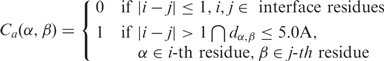
Definition of atom contact (C_a)

Contact between two atoms of the i-th and j-th residues, respectively, is defined as in Equation (1). This equation stipulates that if two atoms are located within a certain cutoff distance, then they are in contact. The cutoff distance between atoms is defined as 5.0 Å (42,43). When deciding whether two atoms are in contact, covalently bonded neighbors are not considered (i.e. for residue i, residues i − 1 and i + 1 are excluded).

1

Here, d_{α, β} is the distance between atoms α and β.

Definition of residue contact (C_r)

Contact between two residues (e.g. the i-th and j-th residues) is defined as in Equation (2), which implies that if there is at least one atom contact between two residues, then we consider that there is one residue contact.

2

Normalized atom contacts (NC_a)

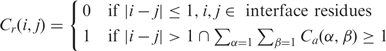
The normalized atom contact at the i-th residue [NC_a(i)] between the i-th and j-th residues is computed by summing all atom contacts between the two residues and dividing by the number of atoms in the i-th residue [N_a(i)], as represented in Equation (3).

3

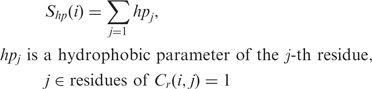
Normalized residue contacts (NC_r)

The normalized residue contact at the i-th residue [NC_r(i)] between the i-th and j-th residues is calculated by summing all residue contacts, as described by Equation (4)

4

Definition of the weighting factor (F_w)

Most studies of protein–protein interactions treat interface residues equally without considering their relative contributions to the total interface area. We believe that this approach may give distorted information about interface residues. In fact the concept of assigning different weights to residues based on their importance in determining system properties has already been used when calculating mean sequence entropy to discriminate oligomerization states of proteins (36). In the present study, this concept is extended to other properties as a weighting factor when quantifying several structural features. The weighting factor, which weights the contribution of each residue according to its relative contribution to the total interface area, is expressed as follows [Equation (5)]:

5

Simple density

Simple density consists of the simple atom density and simple residue density. The simple atom density is defined as the normalized number of atom contacts (NC_a), and the simple residue density is defined as the normalized number of residue contacts (NC_r).

Weighted density

The weighed density is composed of the weighted atomic packing density (W_ad) and weighted residue density (W_rd). The weighted atomic packing density for the i-th residue [W_ad(i)] is obtained by weighting the normalized number of atom contacts [NC_a(i)] using the fraction of ASA buried upon complexation that is due to residue i, as follows [Equation (6)]:

6

Similarly, if we substitute NC_a(i) for NC_r(i), we obtain the weighted residue density for the i-th residue W_rd(i) [Equation (7)]:

7

The differences in weighted density between the bound and monomer states are also computed, which are denoted by △ W_ad(i) and △ W_rd(i).

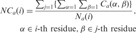
Simple hydrophobicity

To calculate the hydrophobicity, we use the Fauchere and Pliska scale (44) (Supplementary Table S4). The simple hydrophobicity of the i-th residue is defined as follows [Equation (8)]:

8

Weighted hydrophobicity

The weighted hydrophobicity for the i-th residue [W_hp(i)] is obtained by weighting the simple hydrophobicity [S_hp(i)] as follows [Equation (9)]:

9

Relative surface area burial (SB_r)

When dealing with structural properties related to hot spots, most previous studies have focused on conventional concepts such as solvent accessibility and surface area burial (ΔASA). Although these absolute values are useful to describe hot spots, they have only a limited capacity to distinguish hot spots from other interface residues. For example, consider the following two cases: (i) an interface residue having 100 Ų solvent accessibility in the monomer, which is fully buried (0 Ų solvent accessibility) after binding association; (ii) an interface residue having 200 Ų solvent accessibility in the monomer, which has 100 Ų solvent accessibility after binding association. In both cases, the surface area burial (ΔASA) is 100 Ų; However, the relative surface burial in comparison with the solvent accessibility in the monomer differs markedly between the two cases (50% versus 100%). To compensate for this effect, we introduce the concept of relative surface burial. The relative surface burial (SB_r) between the monomer and bound states is calculated as follows:

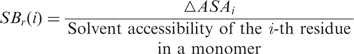10

Residue conservation

To calculate the conservation score, multiple alignment is performed using ClustalW. The conservation score for an interface residue is obtained based on the von Neumann entropy (VNE), which is a modified Shannon entropy (SE) (45). The SE for a multiple alignment position is defined as follows:

11

where p(x) is the relative frequency of each amino acid x in a specific alignment position. The base of 20 ensures that all values are bounded between zero and one. When computing the relative frequency, symbols such as ‘X’, ‘Z’, ‘B’, and ‘-’, are ignored. The VNE is represented by the following extension of the SE:

12

where w is a weighted probability matrix of amino acids in an alignment position, described as follows:

13

The BLOSUM50 similarity matrix is applied; this matrix is reported to be the most favorable one for conservation analysis (45).

Molecular interactions of an interface residue

Eighteen molecular interaction types, which we have defined previously (17), are analyzed on the basis of their occurrences in each interface residue. Canonical hydrogen bonds, noncanonical hydrogen bonds, ion–ion interactions and π–ring system-related interactions are included in this interaction set (46–49).

Molecular interactions within a residue's; microenvironment

To obtain information on the interactions within the microenvironment surrounding a residue, the basic concept of which is from the work of Bagley and Altman on FEATURE (50), we analyzed 18 molecular interaction types within a spherical volume with a radius of 5 Å centered at the residue's; center of mass.

Other features

Other conventional features such as ΔASA and solvent accessibility are also included in this study. In addition, we analyze the sum of the molecular interactions and the sum of the molecular interactions of a residue's; microenvironment.

Data representation

The features are quantified as a feature vector based on the propensities of each feature. The propensities are normalized with the mean and standard deviation of the sample set. The vector representation of the features of an interface residue makes it possible to use classification techniques.

Feature selection

In contrast to other dimensionality reduction techniques such as those based on projection (e.g. principal component analysis) or compression (e.g. information theory), feature selection techniques do not alter the original representation of the input variables. Feature selection techniques thus preserve the original semantics of the variables, thereby enhancing the ability to interpret the experimental results (51). With the aid of feature selection, we can avoid overfitting, improve model performance and provide faster and more cost-effective models. In the present study, feature selection is performed using a decision tree, that shows the best subset of features for discriminating hot spots from other residues.

A decision tree (52) is a tree whose internal nodes are tests on input patterns and whose leaf nodes are categories of patterns. A decision tree assigns a class number to an input pattern by filtering the pattern down through the tests in the tree. Each test has mutually exclusive and exhaustive outcomes.

Two decision trees based on the corresponding training sets (T1, T2) are created using the Treefit function in MATLAB. From these trees, two novel feature sets are developed to create the corresponding SVM models.

Evaluation with SVM

SVM (53) is a classifier based on the similarities between an input pattern and a subset of the training samples. Because it uses a set of training samples called support vectors rather than the whole data set, it shows low complexity and robust output in systems with erroneous data. Due to these characteristics, SVM can be an appropriate candidate for dealing with hot spot data.

To evaluate the selected feature sets, two SVM models are created and tested with 10-fold cross-validation for the training sets (T2, T1). Then, to further validate our models, classification is performed using an independent test set. In this analysis, a Gaussian kernel is used as the kernel function.

Cross-validation

Because it is unclear whether the residues within the same binding interface are independent, a 17-fold ‘leave one protein complex out’ cross-validation is adopted to estimate the performance of our model; this method follows the approach reported by Darnell et al. (29). For each of the 17 protein complexes, we select one protein complex as a test sample, and train our model using the remaining 16 complexes. Then, we test our model using that selected protein complex. While this 17-fold ‘leave one protein complex out’ cross-validation can provide a solution to the inherent dependencies between residues in the same interface, it may cause another problem, known as data size imbalance. The data sizes of the different interfaces are severely unbalanced, which may lead to overfitting. Therefore, we also adopt a 10-fold cross-validation to estimate the performance of our model. The data are randomized before assigning folds, and subdivided into 10 equal partitions. Then, for each of the 10 partitioned groups, we select one as a test sample, train our model using the remaining nine groups, and test the model using the selected group. Both approaches have merits and demerits, and show statistically similar results. In this study, we present the results obtained using 10-fold cross-validation.

Statistical analysis

Mann–Whitney U-test

Statistical analysis along with biological knowledge is used to examine the role of each selected feature. The Mann–Whitney U test (54) is used for the statistical analysis because our sample data do not show a normal distribution, as determined using the Lilliefors test (55), an extension of the Kolmogorov–Smirnov test. The Mann–Whitney U-test is a nonparametric test for assessing whether two samples of observations come from the same distribution. It makes minimal assumptions about the underlying distribution.

We have samples of observations from each of two populations: hot spots (H) and other residues (O) These populations comprise n_H and n_O residues, respectively (n_H = 119, n_O = 146 in T1, and n_H = 65, n_O = 200 in T2). We wish to test the hypothesis that the distribution of measurements in population H is the same as that in population O. The Mann–Whitney U-test is based on ranking the n_H + n_O observations of the combined sample. Each observation has a rank. All sequences of ties are assigned an average rank. The Mann–Whitney U-test statistic is the sum of the ranks for observations from one of the samples. We compute the sum of the ranks for the hot spot population (H), denoted as w_H, and use W_H to represent the corresponding random variable. In our analysis, w_H is in the upper tail; hence P-value = 2pr(w_H ≥ W_H), is obtained using MATLAB.

Paired t-test

To compare the performances of models, the two-tailed, paired t-test is adopted. First, we compute the F1-score of our model for each of 10 partitioned groups in the 10-fold cross-validation process. Then, using the corresponding partitions, we also calculate F1-scores of the other models. Using all 10 paired F1-score sets, we test the statistical significance by examining P-values, obtained using MATLAB. A significance level of 0.05 is used to indicate statistical significance.

RESULTS AND DISCUSSION

The performance of each model is expressed by four measures: sensitivity (i.e. recall), specificity, positively predicted value (i.e. precision) and negatively predicted value. We also compare the performance of each model in terms of the F1-score, which is the harmonic mean of the precision and recall. The F1-score is widely used to handle unbalanced data such as our hot spot data. For a model to be practically meaningful, the F1-score must exceed the fraction of the residues in the data set that are hot spots. The T2 training set consists of 65 hot spots and 200 other residues; hence the F1-score for any model should be >0.25. In the same way, in the case of the T1 training set, composed of 119 hot spots and 146 other residues, the F1-score should be >0.45. For the independent test set, which consists of 127 mutated data, of which 39 are hot spots, the F1-score should be 0.31. As will be shown below, all of the F1-scores of our models are much greater than the above mentioned values, implying that our models are very useful for predicting hot spots. Furthermore, our models show a superior capacity to predict hot spots, compared with previous models such as Robetta (26), FOLDEF (28) and KFC (29). In the following sections, we describe these results in greater detail.

Two novel feature sets

At the initial stage, a total of 54 multifaceted features are designed and quantified. Decision tree analysis is applied to choose the best subset of features from the initial feature set. Decision tree analysis for the two training sets (i.e. T1 or T2), discloses that hot spots can be modeled with only 12 features according to their corresponding training sets, although their constituent features differ slightly depending on the training set. The results are shown in Figure 1. These results are also confirmed by statistical analysis. In both feature sets, newly proposed features such as the weighted atomic packing density (W_ad), relative surface area burial (SB_r) and weighted hydrophobicity (W_hp), are located in the upper level of nodes in the decision tree. This implies that these features are better than other features in discriminating hot spots from other residues. Especially, the weighted atomic packing density shows the best discrimination power. By themselves, interaction features make a minor contribution to distinguishing hot spots from other residues. When combined with other features, however, interaction features assist in classification. The constituent members of the two novel feature sets are listed in the Supplementary Data (Table S5 and S6, respectively).

Figure 1.

Decision tree analyses for the two training sets, T1 (a) and T2 (b). The trees show that hot spots can be modeled using only 12 features according to their corresponding training sets, although the constituent members of the T1- and T2-derived sets differ slightly. In both feature sets, newly proposed features such as the weighted atomic packing density, relative surface area burial and weighted hydrophobicity are located in the upper level of nodes in the decision tree.

Cross-validation with the training sets

Based on the two novel feature sets from T2 and T1, corresponding SVM models are developed and tested with 10-fold cross-validation. Our SVM model is named as MINERVA, an acronym of MINE Residue VAlue. In addition, using the same training sets, three previous methods are also examined, and compared with our SVM models. The classification confusion matrices are listed in Table 2. When T2 is used as a training set, our model shows the best predictive performance (recall = 0.58, precision = 0.73 and F1 = 0.65). These findings indicate that 73% of predicted hot spots are identified as true hot spots (precision), and 58% of the true hot spots are correctly predicted (recall). KFC, which shows the best performance among the previous methods, correctly predicts hot spots with recall = 0.55, precision = 0.58 and F1 = 0.56. The F1-score of our model is higher than that of KFC (ΔF1 = 0.09), a difference that is statistically significant (P = 0.01, paired t-test). This indicates that the predictive performance of our model generated from training set T2 is significantly better than those of the other methods. These results are listed in Table 3.

Table 2.

The classification confusion matrices based on the corresponding training sets (T1,T2)

		Condition
		T1-training set			T2-training set
		Td	Fe	Total	T	F	Total
MINERVAa	Pb	70	24	94	38	14	52
	Nc	49	122	171	27	186	213
	Total	119	146	265	65	200	265
Robetta	P	74	38	112	32	20	52
	N	45	108	153	33	180	213
	Total	119	146	265	65	200	265
FOLDEF	P	57	20	77	19	15	34
	N	62	126	188	46	185	231
	Total	119	146	265	65	200	265
KFC	P	naf	na	na	36	26	62
	N	na	na	na	29	174	203
	Total	na	na	na	65	200	265

^aMINERVA, an acronym of MINE Residue VAlue, is the name of our model.

^bPositive.

^cNegative.

^dTrue.

^eNegative.

^fKFC is only designed to predict hot spots with ΔΔG ≥ 2 kcal/mol, so it is not included in the analysis for the T1 set.

Each column represents the gold standard, and each row represents the class predicted by the model.

Table 3.

Evaluation of the hot spot prediction with T2 using 10-fold cross-validation

	KFC	Robetta	FOLDEF	MINERVA2e
SNa	0.55	0.49	0.32	0.58
SPb	0.85	0.90	0.93	0.89
PPVc	0.58	0.62	0.59	0.73
NPVd	0.88	0.84	0.81	0.87
F1 Score	0.56	0.55	0.41	0.65
ΔF1	**	–	–	0.09
P–value	**	–	–	0.01

^aSensitivity (Recall).

^bSpecificity.

^cPositively predicted value (Precision).

^dNegatively predicted value.

^eThe performance of our model using the 2 kcal/mol training set, T2.

^fMINERVA, an acronym of MINE Residue VAlue, is the name of our model.

When T1 is used as the training set, our model predicts hot spots with recall = 0.59, precision = 0.74 and F1 = 0.66. For this training set, Robetta shows the best performance among the previous methods. KFC is only designed to predict hot spots with ΔΔG ≥ 2 kcal/mol; hence, it is not included in the analysis for the T1 training set. Robetta predicts hot spots performance with recall = 0.62, precision = 0.66 and F1 = 0.64. Although the F1-score of our model is higher than that of Robetta (ΔF1 = 0.02), the difference is not statistically significant (P = 0.70). This indicates that our model shows comparable performance with Robetta. These results establish that our feature-based approach is very useful for predicting hot spots with high confidence, irrespective of the definition of hot spots.

Evaluation with the independent test set

The superior performance of our models is more obvious in the analysis of the independent test set from BID. The F1-scores of our models are 0.52 and 0.57, respectively, for the hot spot definitions of ΔΔG ≥ 1 kcal/mol and ΔΔG ≥ 2 kcal/mol, respectively, while those of the previous methods are in the range of 0.34∼0.40. Because Robetta shows the best predictive performance among the previous methods, we compare our models with Robetta. The F1-scores of our models are much higher than those of Robetta (ΔF1-scores of 0.12 and 0.17; P = 0.004 and 0.0005, respectively, paired t-test). These findings indicate that our models give significantly better predictive performance compared with other methods. The details of our experimental results are listed in Table 4.

Table 4.

Evaluation of the hot spot prediction for each model with the independent test set

	Robetta	KFC	FOLDEF	MINERVA2e	MINERVA1f
SNa	0.33	0.31	0.26	0.44	0.62
SPb	0.87	0.85	0.88	0.90	0.76
PPVc	0.52	0.48	0.48	0.65	0.53
NPVd	0.73	0.74	0.73	0.78	0.82
F1 Score	0.40	0.37	0.34	0.52	0.57
ΔF1	**	–	–	0.12	0.17
P-value	**	–	–	4.31 × 10−3	4.55 × 10−4

^aSensitivity (or recall).

^bSpecificity.

^cPositively predicted value (or precision).

^dNegatively predicted value.

^eThe performance of our model trained with the 2 kcal/mol training set, T2.

^fThe performance of our model trained with the 1 kcal/mol training set, T1.

MINERVA. an acronym of MINE Residue VAlue, is the name of our model.

Weighted density and hot spots

In both of the selected feature sets, the top 3 features showing better discriminating power (i.e. located in the upper level nodes in the decision tree) are the weighted atomic packing density (W_ad), relative surface area burial (SB_r) and weighted hydrophobicity (W_hp). In particular, the weighted atomic packing density (W_ad) is located at the top node in the decision tree. This feature is created using a newly suggested measure that reflects the extent of the contribution of an individual interface residue to the whole interface area.

The weighted atomic packing density (W_ad) in the bound state is compared with the coordination number, a conventional measure (42), in a histogram (Figure 2). The average weighted atom densities of hot spots differ from those of unimportant residues, regardless of the ΔΔG cutoff values, whereas the average coordination numbers of the two groups are very similar (see Table S7 in the Supplementary Data). These findings are supported by the results of a nonparametric statistical analysis, the Mann–Whitney U-test. In agreement with the histogram data, the coordination number does not differ significantly between the two groups, whereas the weighted atomic packing density does show statistically significant difference (Table 5). The P-values for the difference in W_ad are on the order of 10⁻¹¹–10⁻¹², irrespective of the ΔΔG cutoff value. This indicates that the newly suggested concept of the weighted atomic packing density is more efficient than the simple coordination number for distinguishing hot spots from unimportant residues. Our findings that the coordination number does not differ between hot spots and other residues is at odds with previous findings showing that the average coordination number of structurally conserved residues differs from that of the rest of the interface (42). Several factors could potentially explain this discrepancy. In our study, experimentally measured hot spots and other residues are directly compared. In the previous study, in contrast, structurally conserved residues are used in the analysis instead of experimentally measured data, based on the fact that there is a correlation between the propensities of structurally conserved residues and the experimental enrichment of hot spots. However, structurally conserved residues at a protein–protein interaction interface may contribute to structural stability rather than act as hot spots for binding association; hence we cannot say that there is a one-to-one mapping between a hot spot and a structurally conserved residue.

Figure 2.

(a) Weighted atomic packing density in the bound state. (b) Coordination number in the bound state. The weighted atomic packing density is compared with the coordination number using a histogram. The average value of the weighted atomic packing density for hot spots is quite different from that for other residues, irrespective of the ΔΔG cutoff value. In contrast, the coordination number does not differ between hot spots and other residues. This result is supported by statistical analysis (Table 5).

Table 5.

Weighted atomic packing density versus Coordination number

Density type	ΔΔG cutoff value (kcal/mol)	Mann–Whitney U-test, P-values	Hot spotsc/ Othersd
Wada	1.0	3.32 × 10−11	119/146
Wad	2.0	2.22 × 10−12	65/200
CNb	1.0	0.10	119/146
CN	2.0	0.02	65/200

^aWeighted atomic packing density in the bound state.

^bCoordination number in the bound state, defined as the number of C^α within 6.5 Å around each residue (42).

^cNumber of hot spots.

^dNumber of energetically unimportant residues.

The distribution of the weighted atomic packing density in the unbound form of the protein is also analyzed. Here, the ‘unbound form’ indicates a protein that is crystallized as a single monomer in the PDB. In addition, the distribution of the difference of the weighted atomic packing density between before and after binding association (Δ W_ad) is also investigated. To achieve this, we select 12 proteins containing 132 mutation data, which are crystallized in both the unbound and bound forms in the PDB (39). Structural comparisons between the unbound and bound forms, are performed using CE (56) to examine the conformational changes that occur as a result of binding. On the basis of such comparisons, we conclude that the proteins in our data set do not undergo conformational changes when they associate (Table 6). For these 12 proteins, we calculate the weighted atom densities in the unbound and bound forms, and use statistical analysis to compare the findings for hot spots and other residues. The average packing densities of the unbound and bound forms are compared, based on the energetically different types of residues (Figure 3).

Table 6.

Structural comparison between the unbound and bound states for various proteins using combinatorial extension

	Bound statea		Unbound stateb		RMSD(Å)c	Seq.
	PDB id	Chain id	PDB id	Chain id		identity (%)
Angiogenin	1a4y	B	1un3	A	0.76	99.1
hGH	1a22	A	1hgu	–d	2.68	68.4
Tissue factore	1ahw	C	1tfh	A	1.39	100.0
Barnase	1brs	A	1bnf	A	1.12	98.1
Barstar	1brs	D	1a19	A	0.44	98.9
BPTI	1cbw	D	1bpt	–d	0.39	98.2
Tissue factore	1dan	T	1tfh	A	0.63	100.0
RNase inhibitor	1dfj	I	2bnh	–d	1.50	100.0
CD4	1gc1	C	1cdj	A	1.09	100.0
Hen egg lysozymee	1vfb	C	1lyz	–d	1.11	100.0
Trypsin	2ptc	I	1bpt	–d	0.36	98.2
Lysozymee	3hfm	Y	1lyz	–d	0.67	100.0

^aA protein is in the bound state.

^bThese 12 proteins are used for statistical analysis to prove that hot spots already have densely structured organization in the unbound state

^cRoot mean squared error.

^d‘–’ represents that chain id is not presented in the PDB.

^e1ahw C and 1dan T are the same proteins but have different binding sites, and in the same way, 1vfb C, and 3hfm Y have different binding sites.

Figure 3.

(a) The weighted atomic packing density of the hot spots in the unbound state is much higher than the weighted atomic packing density in the rest of the interface. (b) The hot spots are much denser than other residues in the bound state, irrespective of the ΔΔG cutoff value. (c) The difference in weighted atomic packing density between before and after binding association (ΔWAD) is large.

In the bound form of each of 12 proteins, the region around each hot spot is denser than regions that do not contain a hot spot. A similar phenomenon is also observed even in the unbound form. Furthermore, when we analyze the difference in weighted atom packing density between before and after binding association, we find that the difference of the distribution between hot spots and other residues is statistically significant (Table 7). This implies that unbound proteins already have a densely structured organization, and these hot spots are good targets for the interacting partner proteins. These results are in good agreement with those of previous works (33,57,58). Nussinov's; group found that hot spots strongly tend to be complementary pockets that have structures suited to binding with structures in the unbound state (33,57). In a study of anchor residues, Rajamani et al. (58) argued that such residues enable binding pathways that avoid kinetically costly structural rearrangements at the core of the binding interface, thereby creating a relatively smooth recognition process.

Table 7.

P-values for comparisons of distributions of weighted atom densities for energetically different residue types

Density type	ΔΔG cutoff value (kcal/mol)	Mann–Whitney U-test, P values	Hot spotsd/ Otherse
Wbada	2.0	4.24 × 10−11	25/107
	1.0	3.93 × 10−11	49/83
Wuadb	2.0	5.79 × 10−13	25/107
	1.0	2.21 × 10−8	49/83
ΔWadc	2.0	1.88 × 10−8	25/107
	1.0	3.34 × 10−4	49/83

^aW^b_ad : weighted atomic packing density in the bound form.

^bW^u_ad : weighted atomic packing density in the unbound form.

^cΔW_ad : the difference in weighted atom packing density between before and after binding association.

^dNumber of hot spots in the data set.

^eNumber of energetically unimportant residues in the data set.

The interactions between densely packed hot spots are investigated using 3hfm, which is a complex of the proteins HyHEL-10 and lysozyme. The mean and standard deviation of the weighted atomic packing density (W_ad) of the interacting hot spots are 17.34 and 8.27, respectively. In contrast, the corresponding values for the energetically unimportant residues in the interface are 8.55 and 4.80, respectively. These findings clearly show a substantial difference between the two groups of interface residues. These results are presented in the Supplementary Data (Supplementary Table S8). D32, Y33 and Y53 in chain H (HyHEL-10), interact with L75, K97, D101 in chain Y (lysozyme). Y50 and Y58 in chain H interact with Y96 in chain L (HyHEL-10) and R21 in chain Y. Y20 and K96 in chain Y (lysozyme) interact with N31, N32, Y50 and Q53 in chain L (HyHEL-10). These interactions are plotted using a solid 3D representation in Figure 4. In this illustration, the blue spheres represent the hot spots in chain L (HyHEL-10) and the yellow spheres indicate the hot spots in chain H (HyHEL-10). The green spheres are the hot spots in chain Y (Hen egg lysozyme), and the white sticks represent the energetically unimportant residues. The visualizations clearly show that the hot spots with high packing density, interact with each other, and that the energetically unimportant residues are mainly located at the outside of the interface, in good agreement with previous studies (24,60). Similar interaction patterns are also observed in the interfaces between protein pairs (data not shown). These results provide an explanation for why the weighted atomic packing density is located at the topmost node in the decision tree.

Figure 4.

The interactions between densely packed hot spots in 3hfm. D32, Y33 and Y53 in chain H (HyHEL-10), interact with L75, K97, D101 in chain Y (lysozyme). Y53 and Y58 in chain H interact with Y96 in chain L (HyHEL-10) and R21 in chain Y. Y20 and K96 in chain Y interact with N31, N32, Y50 and Q53 in chain L. The blue spheres represent the densely packed hot spots in chain L (HyHEL-10), and the yellow spheres indicate the highly packed hot spots in chain H (HyHEL-10). The green spheres are the highly packed hot spots in chain Y (Hen egg lysozyme), and the white sticks represent the energetically unimportant residues. The images are created by program PyMol (59).

Relative surface area burial (SB_r) and hot spots

The relative surface area burial (SB_r) is also found to be a good feature in the feature selection process, and when combined with other features such as ΔASA and the solvent accessibility, SB_r improves the predictive performance. The Mann–Whitney U-test is used to compare the relative surface area burial (SB_r) of hot spots and other residues. The P-values for this comparison are 3.71 × 10⁻⁹ for data set T1 and 4.11 × 10⁻¹² for data set T2, implying that the distribution of relative surface area burial (SB_r) differs significantly between hot spots and other residues. Therefore, SB_r is selected as one of the top three features showing good discriminating power.

Although solvent accessibility and ΔASA are not among the top three features, these parameters are still major features for distinguishing hot spots from other residues. When ΔΔG ≥ 1.0 kcal/mol is used to define hot spots, there is a statistically significant difference in solvent accessibility between hot spots and the energetically unimportant residues (P = 4.74 × 10⁻⁶, Mann–Whitney U-test). When we use ΔΔG ≥ 2.0 kcal/mol as the hot spot definition, the statistical pattern remains unchanged (P = 1.31 × 10⁻⁷, Mann–Whitney U-test). Comparison of ΔASA values using the Mann–Whitney U-test again shows that the distributions of hot spots and energetically unimportant residues differ significantly. These results are summarized in the Supplementary Data (Table S9).

We now consider the locations of hot spots in an interface. Tryptophan, leucine, isoleucine and valine are mainly located at the center of the interface, with solvent accessibilities ≤10 Ų. In particular, tryptophan shows the highest propensity to be hot spots, owing to its large size and aromatic nature (61). Lysines are mainly located in regions with solvent accessibility ≤20 Ų, although several such residues are found in regions with solvent accessibility ≤70 Ų. This is an unexpected result because lysine is hydrophilic, and hence is likely to be located in the outside of the interface. Arginine, aspartic acid and glutamic acid are mainly located between the center and the edge of the interface, with solvent accessibility ≤80 Ų. Tyrosine is broadly distributed, appearing even in regions with solvent accessibilities in excess of 100 Ų. Arginine is mainly observed between 35 Ų and 75 Ų. These observations show that, to some extent, residues that are more accessible to the solvent can be hot spots. Asparagine, glutamine, serine and threonine exhibit ambiguous behavior. In the case of serine and threonine, the absolute size of the hot spot data is very small. The energetically unimportant residues are broadly distributed regardless of their solvent accessibility. Systematic analysis of hot spots thus discloses that the distinctive amino acids of hot spots are tryptophan, arginine and tyrosine.

Weighted hydrophobicity and hot spots

The weighted hydrophobicity, calculated according to Equation (9), is another of the newly suggested feature to appear among the top three features in the decision tree. Comparison of the distributions of the weighted hydrophobicity between hot spots and energetically unimportant residues reveals statistically significant differences between hot spots and other residues (P = 8.53 × 10⁻⁸ and 3.96 × 10⁻⁹ according to the ΔΔG cutoff values, as shown in Table S10 of the Supplementary Data). As expected, hot spot residues are more hydrophobic than energetically unimportant residues, although the hydrophobicity fluctuates severely throughout the interface (Table 1).

In Figure 5, the relative ratio between hot spots and other residues is plotted according to the weighted hydrophobicity. There is a clear correlation between hydrophobicity and the fraction of residues that are hot spots.

Figure 5.

(a) ΔΔG 1.0 kcal/mol cutoff value. (b) ΔΔG 2.0 kcal/mol cutoff value. Relative ratio between hot spot residues and energetically unimportant residues as a function of the weighted hydrophobicity. As the hydrophobicity increases, the fraction of residues that are hot spots increases.

Conservation and hot spots

In general, hot spots would be expected to be more conserved than other residues. Surprisingly, however, our analysis of conservation scores calculated using VNE indicates that hot spot residues are not more conserved than other residues. Specifically, the P-values of the differences in conservation score between hot spots and other residues are in the range of 0.05–0.79, as shown in Table 8. It may be that antibody–antigen complexes are inappropriate candidates for such evolutionary analysis, because antibodies must mutate and diversify to recognize a variety of antigens. When antibody–antigen complexes are excluded from the analysis, we indeed find that hot spots are more conserved than other residues (P-values in the range of 10⁻³–10⁻⁴). These results are in good agreement with previous studies showing that the interface core is more conserved than the rim (60), and that residue conservation is rarely sufficient for complete and accurate prediction of protein interfaces (45).

Table 8.

P-values from comparisons of distributions of conservation score for energetically different types of residues

	ΔΔG cutoff value (kcal/mol)	Including antibody–antigens		Excluding antibody–antigens
		Mann–Whitney U-test	Hot spotsb/Othersc	Mann–Whitney U-test	Hot spots/Others
VNE	1.0	0.79	119/146	5.10 × 10−3	56/105
	2.0	0.05	65/200	5.36 × 10−4	32/129

^aNumber of hot spots.

^bNumber of energetically unimportant residues.

Molecular interaction information and hot spots

In this study, two general types of interaction information are analyzed: molecular interaction information of an interface residue; and molecular interaction information within a residue's; microenvironment. Eighteen molecular interactions are considered, composed of canonical hydrogen bonds, noncanonical hydrogen bonds, electrostatic interactions and π–ring system-related interactions, all of which are known to be energetically important interactions (17). π–Ring system-related interactions of an interface residue make up the majority of the constituents selected for the feature sets, in good agreement with previous studies indicating that hot spots are often composed of aromatic residues such as tryptophan (W), tyrosine (Y), histidine (H) and phenylalanine (F) (32). Especially, π ··· π interaction is selected as one of the major features in both training sets, T1 and T2. A number of studies have demonstrated that π ··· π interactions play an important role in molecular recognition (46,62). In T2, there are a total of 70 aromatic residues, and 24 of which are hot spots and 46 of which are energetically unimportant residues. Of the 24 aromatic residue, 21 hot spots have at least one π ··· π interaction, reaching 87.5% of hot spots, and the remaining three hot spots have π ···Cation interactions. Of the 46 energetically unimportant residues, only 16 have π ··· π interactions. These results show that π ··· π interactions are a characteristic feature of hot spot residues. These findings are supported by the statistical analysis, in which the P-value for the difference between hot spots and other residues is 5.95 × 10⁻⁹.

The molecular interaction information is located in a lower level of nodes in the decision tree; hence, the structural features dominate the bonding/electrostatic interactions.

CONCLUSIONS

In the study of protein–protein interactions, experimental identification of binding hot spots is time-consuming and labor-intensive effort; thus, the development of predictive models can be very helpful. A good predictive model requires features that effectively represent the energetic contributions of individual interface residues to the binding association. A number of studies have sought to identify such features; however, the features previously identified as being positively correlated with hot spots are still insufficient to accurately predict hot spots. Therefore, feature-based approaches have been proceeded with very limited scope.

In the present study, we propose several new features quantified by a new measure, and show that these features are more effective than conventional features. By combining the proposed and the conventional features, we develop two predictive SVM models for predicting interaction hot spots. The performance of our models is first evaluated through 10-fold cross-validation with two training sets from 265 alanine-mutated interfaces residues, and then further validation is performed with an independent test set from the BID. Our models clearly show better overall predictive performance than previous methods, a finding supported by statistical analysis. In the independent test set, the F1-scores of our models are 0.52 and 0.57 for training sets T2 and T1, respectively. When these results are compared with those of Robetta (F1 = 0.40), which shows the best performance among the previous methods, our models exhibit a statistically significant increase in overall predictive accuracy for hot spots (P = 4.31 × 10⁻³ and 4.55 × 10⁻⁴, respectively).

The present results imply that the energetic properties of the interface residues are well reflected in our selected features. Statistical analysis shows that in the bound state, the density distribution of hot spots differs significantly from that of other residues. Even in the unbound state, this phenomenon is maintained. This implies that unbound proteins already contain densely structured regions suitable for interaction with partner proteins, and that these structured hot spots can be good targets for interacting partners. This phenomenon is difficult to discern using the coordination number (the simple frequency of C^α atoms around hot spots) as a density measure, even though this parameter is known to be positively correlated with hot spots. The coordination number distribution of hot spots does not differ significantly from that of other residues. The regions around these densely packed hot spots are more hydrophobic than the other regions, and the hot spots have larger relative surface area burial compared with other residues. Unexpectedly, hot spot residues are not more conserved than other residues. However, when antibody–antigen complexes are excluded from the analysis, the hot spots are more conserved than other residues. This is reasonable if we consider that antibodies must mutate their sequences for recognizing a variety of antigens, and hence may not be appropriate candidates for evolutionary analysis.

Unlike previous models, we incorporate molecular interaction information into our models, allowing us to analyze the relationship between molecular interactions and hot spots. Interestingly, our models show that hot spots are closely related to the π-related interactions, especially π ··· π interactions.

The question of which residues are energetically more important in protein–protein interaction interfaces is a long-standing issue. Although a number of studies have addressed this question, the identification of hot spot residues remains a difficult task. Studies solely based on structural features are confined to examining the solvent accessibility or surface area burial between the unbound and bound states, and studies based on thermodynamics still show large discrepancies between predicted and experimentally measured free energy changes, although they are very useful in understanding the stability and folding processes of proteins. Accordingly, new features that well describe the different energetic contributions to binding interactions are still greatly needed. The new features proposed in this work should assist in understanding the binding process, and in predicting hot spots with high accuracy. In the near future, we will make available a web-based interface through which our models can be run to predict hot spots.

SUPPLEMENTARY DATA

Supplementary Data are available at NAR Online.

FUNDING

This work was supported by the Korean System Biology Program (No. M10309020000-03B5002-00000), the National Research Lab. Program (No. 2006-01508), and the Pioneer Research Program for Converging Technology from MEST through KOSEF. Funding for open access charge: Pioneer Research Program for Converging Technology.

Conflict of interest statement. None declared.

REFERENCES

- 1.Salwinski L, Eisenberg D. Computational methods of analysis of protein-protein interactions. Curr. Opin. Struct. Biol. 2003;13:377–382. doi: 10.1016/s0959-440x(03)00070-8. [DOI] [PubMed] [Google Scholar]
- 2.Aloy P, Russell RB. Ten thousand interactions for the molecular biologist. Nat. Biotechnol. 2004;22:1317–1321. doi: 10.1038/nbt1018. [DOI] [PubMed] [Google Scholar]
- 3.Chothia C, Janin J. Principles of protein-protein recognition. Nature. 1975;256:705–708. doi: 10.1038/256705a0. [DOI] [PubMed] [Google Scholar]
- 4.Argos P. An investigation of protein subunit and domain interfaces. Protein Eng. 1988;2:101–113. doi: 10.1093/protein/2.2.101. [DOI] [PubMed] [Google Scholar]
- 5.Janin J, Chothia C. The structure of protein-protein recognition sites. J. Biol. Chem. 1990;265:16027–16030. [PubMed] [Google Scholar]
- 6.Korn AP, Burnett RM. Distribution and complementarity of hydropathy in multisubunit proteins. Proteins Struct. Funct. Genet. 1991;9:37–55. doi: 10.1002/prot.340090106. [DOI] [PubMed] [Google Scholar]
- 7.Lawrence MC, Colman PM. Shape complementarity at protein/protein interfaces. J. Mol. Biol. 1993;234:946–950. doi: 10.1006/jmbi.1993.1648. [DOI] [PubMed] [Google Scholar]
- 8.Jones S, Thornton JM. Protein-protein interactions: A review of protein dimer structures. Prog. Biophys. Molec. Biol. 1995;63:31–65. doi: 10.1016/0079-6107(94)00008-w. [DOI] [PubMed] [Google Scholar]
- 9.Jones S, Thornton JM. Principles of protein-protein interactions. Proc. Natl Acad. Sci. USA. 1996;93:13–20. doi: 10.1073/pnas.93.1.13. [DOI] [PMC free article] [PubMed] [Google Scholar]
- 10.Jones S, Thornton JM. Analysis of protein-protein interaction sites using surface patches. J. Mol. Biol. 1997;272:121–132. doi: 10.1006/jmbi.1997.1234. [DOI] [PubMed] [Google Scholar]
- 11.McCoy AJ, Epa VA, Colman PM. Electrostatic complementarity at protein/protein interfaces. J. Mol. Biol. 1997;268:570–584. doi: 10.1006/jmbi.1997.0987. [DOI] [PubMed] [Google Scholar]
- 12.LoConte L, Chothia C, Janin J. The atomic structure of protein-protein recognition sites. J. Mol. Biol. 1999;285:2177–2198. doi: 10.1006/jmbi.1998.2439. [DOI] [PubMed] [Google Scholar]
- 13.Nooren IMA, Thornton JM. Structural characterization and functional significance of transient protein-protein interactions. J. Mol. Biol. 2003;325:991–1018. doi: 10.1016/s0022-2836(02)01281-0. [DOI] [PubMed] [Google Scholar]
- 14.Keskin O, Bahar I, Badretdinov AY, Ptitsyn OB, Jernigan RL. Empirical solvent-mediated potentials hold for both intra-molecular and inter-molecular inter-residue interactions. Protein Sci. 1998;7:2578–2586. doi: 10.1002/pro.5560071211. [DOI] [PMC free article] [PubMed] [Google Scholar]
- 15.Glaser F, Steinberg DM, Vakser IA, Ben-Tal N. Residue frequencies and pairing preferences at protein-protein interfaces. Proteins Struct. Funct. Genet. 2001;43:89–102. [PubMed] [Google Scholar]
- 16.Mintseris J, Weng Z. Structure, function and evolution of transient and obligate protein-protein interactions. Proc. Natl Acad. Sci. USA. 2005;102:10930–10935. doi: 10.1073/pnas.0502667102. [DOI] [PMC free article] [PubMed] [Google Scholar]
- 17.Kyu-il C, Kiyoung L, Kwang HL, Dongsup K, Doheon L. Specificity of molecular interactions in transient protein-protein interaction interfaces. Proteins Struct. Funct. Genet. 2006;65:593–606. doi: 10.1002/prot.21056. [DOI] [PubMed] [Google Scholar]
- 18.DeLano WL, Ultsch MH, de Vos AM, Wills JA. Convergent solutions to binding at a protein-protein interface. Science. 2000;287:1279–1283. doi: 10.1126/science.287.5456.1279. [DOI] [PubMed] [Google Scholar]
- 19.DeLano WL. Unraveling hot spots in binding interfaces: progress and challenges. Curr. Opin. Struct. Biol. 2002;12:14–20. doi: 10.1016/s0959-440x(02)00283-x. [DOI] [PubMed] [Google Scholar]
- 20.Wells JA. Systematic mutational analyses of protein-protein interfaces. Methods Enzymol. 1991;202:390–411. doi: 10.1016/0076-6879(91)02020-a. [DOI] [PubMed] [Google Scholar]
- 21.Clackson T, Wells JA. A hot spot of binding energy in a hormone-receptor interface. Science. 1995;267:383–386. doi: 10.1126/science.7529940. [DOI] [PubMed] [Google Scholar]
- 22.Clackson T, Ultsch MH, Wells JA, de Vos AM. Structural and functional analysis of the 1:1 growth hormone:receptor complex reveals the molecular basis for receptor affinity. J. Mol. Biol. 1998;277:1111–1128. doi: 10.1006/jmbi.1998.1669. [DOI] [PubMed] [Google Scholar]
- 23.Thorn KS, Bogan AA. ASEdb: a database of alanine mutations and their effects on the free energy of binding in protein interactions. Bioinformatics. 2001;17:284–285. doi: 10.1093/bioinformatics/17.3.284. [DOI] [PubMed] [Google Scholar]
- 24.Bogan AA, Thorn KS. Anatomy of hot spots in protein interfaces: characterization and comparison with oligomeric protein interfaces. J. Mol. Biol. 1998;280:1–9. doi: 10.1006/jmbi.1998.1843. [DOI] [PubMed] [Google Scholar]
- 25.Massova I, Kollman PA. Computational alanine scanning to probe protein-protein interactions: a novel approach to evaluate binding free engergies. J. Am. Chem. Soc. 1999;121:8133–8143. [Google Scholar]
- 26.Kortemme T, Kim DE, Baker D. Computational alanine scanning of protein-protein interfaces. Sci. STKE. 2004;219:pl2. doi: 10.1126/stke.2192004pl2. [DOI] [PubMed] [Google Scholar]
- 27.Kortemme T, Baker D. A simple physical model for binding energy hot spots in protein-protein complexes. Proc. Natl Acad. Sci. USA. 2002;99:14116–14121. doi: 10.1073/pnas.202485799. [DOI] [PMC free article] [PubMed] [Google Scholar]
- 28.Guerois R, Nielsen JE, Serrano L. Predicting changes in the stability of proteins and protein complexes: a study of more than 1000 mutations. J. Mol. Biol. 2002;320:369–387. doi: 10.1016/S0022-2836(02)00442-4. [DOI] [PubMed] [Google Scholar]
- 29.Darnell SJ, Page D, Mitchell JC. An automated decision-tree approach to predicting protein interaction hot spots. Proteins Struct. Funct. Bioinform. 2007;68:813–823. doi: 10.1002/prot.21474. [DOI] [PubMed] [Google Scholar]
- 30.Darnell SJ, LeGault L, Mitchell JC. KFC Server: interactive forecasting of protein interaction hot spots. Nucleic Acids Res. 2008;36:W265–W269. doi: 10.1093/nar/gkn346. [DOI] [PMC free article] [PubMed] [Google Scholar]
- 31.Hu Z, Ma B, Wolfson H. Conservation of polar residues as hot spots at protein interfaces. Proteins Struct. Funct. Genet. 2000;39:331–342. [PubMed] [Google Scholar]
- 32.Ma B, Elkayam T, Wolfson H, Nussinov R. Protein-protein interactions: structually conserved residues distinguish between binding sites and exposed protein surfaces. Proc. Natl Acad. Sci. USA. 100:5772–5777. doi: 10.1073/pnas.1030237100. [DOI] [PMC free article] [PubMed] [Google Scholar]
- 33.Haliloglu T, Keskin O, Ma B, Nussinov R. How similar are protein folding and protein binding nuclei? Examination of vibrational motions of energy hot spots and conserved residues. Biophys. J. 2005;88:1552–1559. doi: 10.1529/biophysj.104.051342. [DOI] [PMC free article] [PubMed] [Google Scholar]
- 34.Halperin I, Wolfson H, Nussinov R. Protein-protein interactions: coupling of structurally conserved residues and of hot spots across interfaces. Implications for docking. Structure. 12:1027–1038. doi: 10.1016/j.str.2004.04.009. [DOI] [PubMed] [Google Scholar]
- 35.Fischer T, Arunachalam K, Bailey D, Mangual V, Bakhru S, Russo R, Huang D, Paczkowski M, Lalchandani V, Ramachandra C, et al. The binding interface database (BID): a compilation of amino acid hot spots in protein interfaces. Bioinformatics. 2003;19:1453–1454. doi: 10.1093/bioinformatics/btg163. [DOI] [PubMed] [Google Scholar]
- 36.Elcock AH, McCammon JA. Identification of protein oligomerization states by analysis of interface conservation. Proc. Natl Acad. Sci. USA. 2001;98:2990–2994. doi: 10.1073/pnas.061411798. [DOI] [PMC free article] [PubMed] [Google Scholar]
- 37.Toth G, Watts CR, Murphy RF, Lovas S. Significance of aromatic-backbone amide interactions in protein structure. Proteins Struct. Funct. Genet. 2001;43:373–381. doi: 10.1002/prot.1050. [DOI] [PubMed] [Google Scholar]
- 38.Pearl FM, Todd A, Sillitoe I, Dibley M, Redfern O, Lewis T, Bennett C, Marsden R, Grant A, Lee D, et al. The CATH domain structure database and related resources Gene3D and DHS provide comprehensive domain family information for genome analysis. Nucleic Acids Res. 2005;33:D247–D239. doi: 10.1093/nar/gki024. [DOI] [PMC free article] [PubMed] [Google Scholar]
- 39.Berman HM, Westbrook J, Feng Z, Gilliland G, Bhat TN, Weissig H, Shindyalov IN, Bourne PE. The protein data bank. Nucleic Acids Res. 28:235–242. doi: 10.1093/nar/28.1.235. [DOI] [PMC free article] [PubMed] [Google Scholar]
- 40.Andreeva A, Howorth D, Brenner SE, Hubbard TJP, Chothia C, Murzin AG. SCOP database in 2004: refinements integrate structure and sequence family data. Nucleic Acids Res. 2004;32:D226–D229. doi: 10.1093/nar/gkh039. [DOI] [PMC free article] [PubMed] [Google Scholar]
- 41.Collaborative Computational Project, Number 4. The CCP4 Suite: programs for protein crystallography. Acta Cryst. 1994;D50:760–763. doi: 10.1107/S0907444994003112. [DOI] [PubMed] [Google Scholar]
- 42.Keskin O, Ma B, Nussinov R. Hot regions in protein-protein interactions: the organization and contribution of structurally conserved hot spot residues. J. Mol. Biol. 2005;345:1281–1294. doi: 10.1016/j.jmb.2004.10.077. [DOI] [PubMed] [Google Scholar]
- 43.del Sol A, Fujihashi H, Amoros D, Nussinov R. Residue centrality, functionally important residues and active site shape: analysis of enzyme and non-enzyme families. Protein Sci. 2006;15:2120–2128. doi: 10.1110/ps.062249106. [DOI] [PMC free article] [PubMed] [Google Scholar]
- 44.Fauchere JL, Pliska V. Hydrophobic parameters pi of amino-acid side chains from the partitioning of N-acetyl-amino-acid amides. J. Eur. Med. Chem. 1983;18:369–375. [Google Scholar]
- 45.Caffrey DR, Somaroo S, Hughes JD, Mintseris J, Huang ES. Are protein-protein interfaces more conserved in sequence than the rest of the protein surface? Protein Sci. 13:190–202. doi: 10.1110/ps.03323604. [DOI] [PMC free article] [PubMed] [Google Scholar]
- 46.Steiner T, Koellner G. Hydrogen bonds with π-acceptors in proteins: frequencies and role in stabilizing local 3D structures. J. Mol. Biol. 2001;305:535–557. doi: 10.1006/jmbi.2000.4301. [DOI] [PubMed] [Google Scholar]
- 47.Gallivan JP, Dougherty DA. Cation-π interactions in structural biology. Proc. Natl Acad. Sci. USA. 1999;96:9459–9464. doi: 10.1073/pnas.96.17.9459. [DOI] [PMC free article] [PubMed] [Google Scholar]
- 48.Jiang L, Lai L. CH—O Hydrogen bonds at protein-protein interfaces. J. Biol. Chem. 2002;227:37732–37740. doi: 10.1074/jbc.M204514200. [DOI] [PubMed] [Google Scholar]
- 49.Baker E, Hubbard R. Hydrogen bonding in globular proteins. Prog. Biophy. Mol. Biol. 1984;44:97–179. doi: 10.1016/0079-6107(84)90007-5. [DOI] [PubMed] [Google Scholar]
- 50.Bagley SC, Altman RB. Characterizing the microenvironment surrounding protein sites. Protein Sci. 1995;4:622–635. doi: 10.1002/pro.5560040404. [DOI] [PMC free article] [PubMed] [Google Scholar]
- 51.Saeys Y, Inza I, Larrañaga P. A review of feature selection techniques in bioinformatics. Bioinformatics. 2007;23:2507–2517. doi: 10.1093/bioinformatics/btm344. [DOI] [PubMed] [Google Scholar]
- 52.Nilsson NJ Stanford University. Introduction to Machine Learing. 1996. [(accessed on 2nd January, 2009)]. pp. 81–96. http://robotics.stanford.edu/people/nilsson/mlbook.html.
- 53.Noble WS. What is a support vector machine? Nat. biotechnol. 2006;24:1565–1567. doi: 10.1038/nbt1206-1565. [DOI] [PubMed] [Google Scholar]
- 54.Mann HB, Whitney DR. On a test of whether one of two random variables is stochastically larger than the other. Ann. Math. Stat. 1947;18:50–60. [Google Scholar]
- 55.Lilliefors H. On the Kolmogorov-Smirnov test for normality with mean and variance unknown. JASA. 1967;62:399–402. [Google Scholar]
- 56.Shindyalov AN, Bourne PE. Protein structure alignment by incremental combinatorial extension (CE) of the optimal path. Protein Eng. 1998;9:739–747. doi: 10.1093/protein/11.9.739. [DOI] [PubMed] [Google Scholar]
- 57.Li X, Keskin O, Ma B, Nussinov R, Liang J. Protein-protein interactions: hot spots and structurally conserved residues often locate in complemented pockets that pre-organized in the unbound states: implications for docking. J. Mol. Biol. 2004;344:781–795. doi: 10.1016/j.jmb.2004.09.051. [DOI] [PubMed] [Google Scholar]
- 58.Rajamani D, Thiel S, Vajda S, Camacho CJ. Anchor residues in protein–protein interactions. Proc. Natl Acad. Sci. USA. 2004;101:11287–11292. doi: 10.1073/pnas.0401942101. [DOI] [PMC free article] [PubMed] [Google Scholar]
- 59.Delano WL. Palo Alto, CA: DeLano Scientific; 2002. The PyMOL Molecular Graphics System. [Google Scholar]
- 60.Guharoy M, Chakrabati P. Conservation and relative importance of residues across protein-protein interfaces. Proc. Natl Acad. Sci. USA. 2005;102:15447–15452. doi: 10.1073/pnas.0505425102. [DOI] [PMC free article] [PubMed] [Google Scholar]
- 61.Moreira IS, Fernandes PA, Ramos MJ. Hot spots–a review of the protein-protein interface determinant amino-acid residues. Proteins. 2007;68:803–812. doi: 10.1002/prot.21396. [DOI] [PubMed] [Google Scholar]
- 62.McGaughey GB, Gagné M, Rappé AK. π–stacking interactions: alive and well in proteins. Proteins. 1998;273:15458–15463. doi: 10.1074/jbc.273.25.15458. [DOI] [PubMed] [Google Scholar]
Associated Data
This section collects any data citations, data availability statements, or supplementary materials included in this article.