Characterizing multiple independent behavioral correlates of cell firing in freely moving animals

Abstract

The heterogeneous sampling of behavioral states by freely moving animals hinders our ability to relate neuronal firing rates to behavioral variables by introducing dependencies between them. We specifically consider the animal’s location and orientation, although our analyses may generalize to other behavioral variables such as speed of movement. A maximum-likelihood approach is presented for producing estimates of the separate histograms relating firing rate to multiple independent causes. Examples show that the method can be used to avoid the artefactual behavioral correlates of place and head-direction cell firing produced by standard analyses; to characterize the independent influences of both location and orientation in a third cell type (Cacucci at al., submitted); and to demonstrate the location-independence of the directional firing of head-direction cells.

There are good examples of surprisingly pure firing-rate responses to an animal’s location and orientation: ‘place cells’ fire at a high rate whenever the animal is in a specific portion of its environment (the ‘place field’ O’Keefe & Dostrovsky, 1971; O’Keefe, 1976), while ‘head-direction cells’ fire whenever the animal’s head is pointing in a specific direction (Taube, Muller, & Ranck, Jr., 1990). In standard analyses the experimenter collects the number of spikes fired by a putative single neuron and the ‘dwell time’ spent by the animal corresponding to different intervals (‘bins’) in the range of the behavioral variable in question. A histogram of the firing rate (number of spikes divided by dwell time) as a function of the behavioral variable is then produced, and often smoothed for interpretability using a fixed (O’Keefe & Burgess, 1996) or variable (Markus et al., 1995) sized kernel.

However, inhomogeneous sampling of behavioral variables by the animal’s motion creates dependencies amongst them which can produce artefactual results. For example, inhomogeneity in the sampling of orientations will cause place cell firing to show an apparent preferential response to those head-directions sampled most frequently when the animal is in the place field. Likewise, inhomogeneity in the sampling of places will cause head-direction cells to show an apparent preferential response to those places sampled most frequently with the preferred head-direction. Inhomogeneity of sampling is unavoidable in freely moving animals, and is often particularly acute at the boundaries of an environment, where locations can only be approached in particular directions. In this paper we present a method for estimating the effect of one variable (e.g. location) on firing rate while taking into account the effect of a second variable (e.g. orientation).

Suppose we are interested in the independent modulatory influences on firing rate as a function of location x divided into N_l bins centered on the positions x_i and head direction θ divided into N_d bins centered on directions θ_j. Our data consist of the number of spikes n_ij and the ‘dwell time’ t_ij corresponding to locations x_i and directions θ_j. The traditional spatial firing rate map would be defined as f(x_i) = n_i/t_i, where n_i = Σ_j n_ij and t_i = Σ_j t_ij are the number of spikes and dwell time in the location bin at x_i. Similarly, the traditional directional firing rate polar plot would be defined as f(θ_j) = n_j/t_j, where n_j = Σ_i n_ij and t_j = Σ_i t_ij are the number of spikes and dwell time in the direction bin at θ_j.

The presence of a directional effect on place cell firing beyond the artefactual effect of inhomogeneous behavior interacting with a ‘true’ locational effect can be detected using the ‘distributive hypothesis’ (Muller, Bostock, Taube, & Kubie, 1994). The directional firing predicted by the ‘Null’ hypothesis (no influence of direction other than that caused by a locational effect) is calculated. Thus the assumed ‘true’ locational firing rate map f(x_i) = n_i/t_i is attributed to directions according to the time spent facing in each direction at each location to produce the predicted artefactual dependence on direction:

$$f^{\prime }\left({\theta }_j\right)={\Sigma }_i{t}_{ij}(n_i∕t_i)∕{\Sigma }_i{t}_{ij}$$ (1)

The observed firing rate polar plot f(θ_j) can then be tested to see if it differs significantly from f ’(θ_j). This was successfully used to show that place cell firing in an open cylinder was not directionally modulated (i.e. f(θ_j) did not differ significantly from f ’(θ_j), Muller et al., 1994). A similar procedure could be used to detect the presence of a locational effect beyond that due to inhomogeneous behavior interacting with a ‘true’ directional effect. In addition, semi-partial correlation coefficients can be used to describe the amount of overall variance accounted for by one variable after taking into account the effects of other variables (Sharp, 1996). However, these procedures do not allow estimation and visualization of the relative effects of location and direction in cells for which there might be ‘true’ effects of both.

We now outline how the parameters of a model of independent modulatory influences on firing rate can be estimated. Under such a ‘factorial’ model, the expected number of spikes per location and direction bin is parameterized as:

$$\mathrm{E}\left(n_{ij}\right)=p_i{d}_j{t}_{ij},$$ (2)

where p_i represents the contribution of position x_i as a cause of firing and d_j represents the contribution of direction θ_j as a cause of firing. The maximum-likelihood approach (see e.g. Duda, Hart, & Stork, 2001) is to choose p_i and d_j to maximize the probability of the observed data n_ij under the model. For this we must define a probability distribution for the observed data, not just the expected values. The most obvious choice for the number of counts per bin of a random variable is the Poisson distribution. While this seems a reasonable model for firing as a function of position or direction, it would not be such a good model for firing as a function of time. Fenton and Muller (1998) note that, in contrast to the reliability of place cell firing as a function of location, averaged over several runs (i.e. n_i/t_i above), the firing rate on individual runs through a place field shows greater variability than consistent with a Poisson distribution. One reason for this might be that rate covaries with factors other than location, e.g. speed, which average out over many runs. The likelihood of the data in a single bin under a Poisson model is:

$$\mathrm{p}(n_{ij}\mid p_i,d_j,t_{ij})={\left({\lambda }_{ij}\right)}^{n_{ij}}\exp (-{\lambda }_{ij})∕n_{ij}!$$ (3)

where λ_ij = p_i d_j t_ij under the factorial model. Assuming independence over bins, the likelihood of the data L and the log likelihood l are, respectively:

$$L={\Pi }_{ij}\mathrm{p}(n_{ij}\mid p_i,d_j,t_{ij}),\text{and}l={\Sigma }_{ij}\log \left(\mathrm{p}(n_{ij}\mid p_i,d_j,t_{ij})\right).$$ (4)

Under the factorial model with Poisson noise:

$$l={\Sigma }_{ij}{n}_{ij}\log \left({\lambda }_{ij}\right)-{\lambda }_{ij}-\log (n_{ij}!)={\Sigma }_{ij}{n}_{ij}\log \left(p_i{d}_j{t}_{ij}\right)-p_i{d}_j{t}_{ij}-\log (n_{ij}!).$$ (5)

By setting the partial derivatives ∂l/∂p_i and ∂l/∂d_j equal to zero we see that the values of p_i and d_j that maximize l (and thus maximize L) obey:

$$p_i={\Sigma }_j{n}_{ij}∕{\Sigma }_j{d}_j{t}_{ij};d_j={\Sigma }_i{n}_{ij}∕{\Sigma }_i{p}_i{t}_{ij}.$$ (6)

These N_l + N_d equations can be iterated¹ to find p_i and d_j, given a sufficiently large number of data points n_ij (in principle there can be N_l×N_d observations of n_ij but in practice far fewer are sampled and many of these will be zero). Intuitively the equations can be thought of as setting d_j to be the multiplicative factor by which the observed number of spikes for direction θ_j differs from that predicted by the locational firing pattern (using a distributive hypothesis) and vice versa for p_i. To display p_i or d_j independently of the other, as estimated firing rate plots, the values in each plot are scaled so as to match the total numbers of spikes recorded.

We next illustrate the use of our approach in assessing the effects of location and direction on cell firing, as compared to simply composing histograms relating firing rate to location or direction without consideration of the effects of one variable on the other. The cells shown were recorded using tetrodes (Recce & O’Keefe, 1989) from freely moving rats exploring for scattered food rewards in walled environments (see e.g. Lever, Wills, Cacucci, Burgess, & O’Keefe, 2002 for methods). The animal’s location and head-direction is tracked by an overhead camera monitoring two LEDs (one bright, one dim) on the animal’s head (Axona, ltd.).

Figure 1 shows examples of the firing of head-direction cells in the presubiculum displayed as uncorrected histograms of the directional and locational effects (uncorr) or when the combined maximum likelihood model is used to correct for the effects of direction and location on each other (corr, equation 6). Note the spurious positional correlate of firing in the uncorrected histogram by position, due to the preferred head-direction occurring preferentially in locations near to the edge of the environment (e.g. HD1 where the rat tends to approach the north edge facing northwards, and HD2-3 where it shows some unidirectional wall-following). These do not occur when using the combined maximum likelihood model. As noted in the caption, applying the combined model tends to noticeably reduce the locational information content of the firing of these cells, but not so the directional information content (as estimated by the method of Skaggs, McNaughton, & Gothard, 1993). In a larger sample of 43 head-direction cells, locational information (in bits per spike) was reduced by 28% on average while directional information was reduced by 4%. However the specific effect of the correction on a given cell was by no means uniform (standard deviation of reduction of information: 25% for location; 7% for direction).

Figure 1.

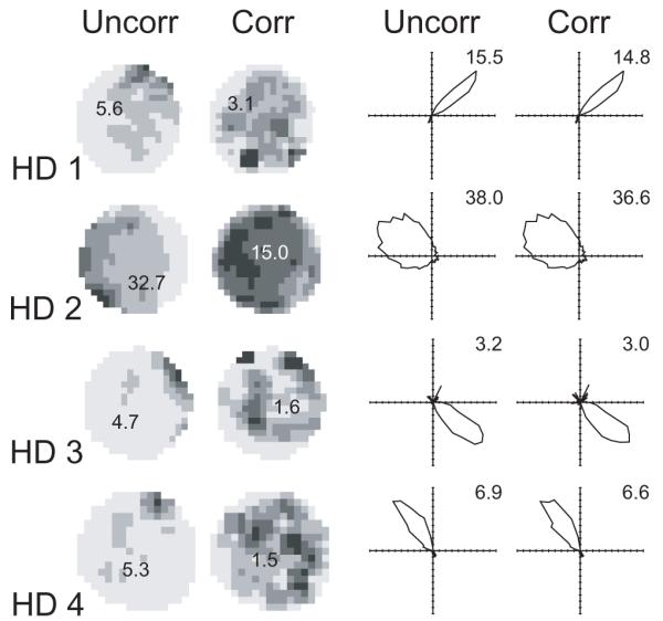
The firing rate histograms of 4 ‘head-direction cells’ (HDs) recorded over 10 minutes. Left hand columns show locational rate histograms. Righthand columns show directional rate histograms. The peak firing rate (Hz) is shown on each plot. Uncorr shows the uncorrected histograms which simply plot the number of spikes divided by dwell time in each interval in the corresponding behavioral variable. Corr shows the histograms calculated under the maximum likelihood factorial model (MLM, equation 6) to correct for the effects of direction and location on each other. Note the spurious positional effects shown using the uncorrected histograms. Applying MLM decreases locational information content (from uncorr to corr: 0.32 to 0.22, 0.18 to 0.04, 0.75 to 0.40, 0.35 to 0.21 bits per spike in cells 1 to 4 respectively, see also main text) and decreases locational peak rates, but produces similar directional information content (2.33 to 2.28, 0.63 to 0.60, 1.61 to 1.50, 1.93 to 1.97 in cells 1 to 4 respectively) and directional peak rates. To give reasonable spatial resolution and interpretability, binning of locations uses a square grid such that on average 245 locational bins were occupied (i.e. mean N_l = 245) and locational histograms were smoothed using a 3×3 kernel. Directions were divided into 60 bins (nearly always fully occupied, i.e. N_d = 60) and directional plots were not smoothed.

Figure 2 shows examples of the firing of hippocampal place cells displayed as uncorrected histograms of the directional and positional effects (uncorr) or when the combined model is used (corr). Note the spurious directional correlate of firing observed in the uncorrected histogram by direction. Spurious peaks in the directional histogram occur at the directions along which the rat most often ran through the place field. This spurious directionality is reduced in the combined model. As noted in the caption, applying the combined model noticeably reduced the directional information content of the firing of these cells, but not so the locational information content. In a larger sample of 44 place cells, directional information (in bits per spike) was reduced by 27% on average (standard deviation 21%) while locational information was increased by 1% (standard deviation 10%).

Figure 2.

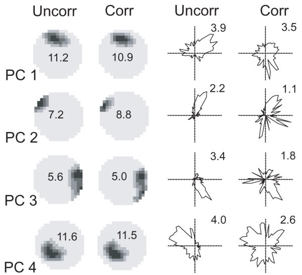
The firing rate histograms of 4 ‘place cells’ (PCs) simultaneously recorded over 20 minutes. Left hand columns show locational rate histograms. Righthand columns show directional rate histograms. Uncorr columns show the uncorrected separate histograms while Corr columns show the histograms calculated under the maximum likelihood factorial model (MLM), as in Figure 1. Note the spurious directional effects shown using the uncorrected separate histogram. Applying the MLM decreases directional information content (from uncorr to corr: 0.27 to 0.08, 0.98 to 0.51, 0.73 to 0.28, 0.29 to 0.07 in cells 1 to 4 respectively) and directional peak rates, but produces similar locational information content (1.66 to 1.71, 3.12 to 3.26, 1.77 to 1.70, 1.57 to 1.58 in cells 1 to 4 respectively) and locational peak rates.

Figure 3 shows examples of a third cell type recorded in the pre- and para-subiculum (Cacucci et al., submitted) which has a genuine response to both place and direction, as shown by the combined model. Note the spurious ‘edge field’ in the uncorrected histogram by position for TPD1. Figure 4 demonstrates the anecdotally well-known fact that the directional preference of head-direction cells is independent of position. Using uncorrected histograms over direction to make this point would be open to doubt due to differences in the sampling of head-directions in the different parts of the environment.

Figure 3.

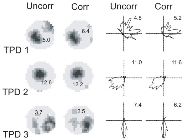
The firing rate histograms of 3 ‘theta-modulated place-by-direction cells’ (TPD; Cacucci et al., submitted) recorded over 10 minutes. Left hand columns show locational rate histograms. Righthand columns show directional rate histograms. Uncorr columns show the uncorrected separate histograms while Corr columns show the histograms calculated under the maximum likelihood factorial model (MLM), as in Figure 1. The MLM allows an unbiased picture of the dependencies on place and direction to be shown. Note the spurious positional effect at the edge of the environment using the uncorrected histogram in cell 1. The precise effect of applying the MLM on peak rates and information content cannot be simply predicted (locational information, from uncorr to corr: 0.47 to 0.67, 0.93 to 0.87, 0.74 to 0.60 in cells 1 to 3 respectively; directional: 0.42 to 0.63, 0.85 to 0.78, 1.86 to 1.54 in cells 1 to 3 respectively).

Figure 4.

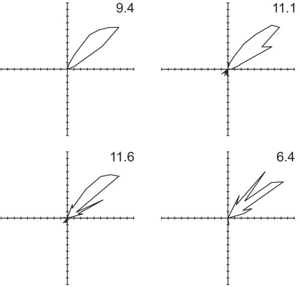
The effect of head-direction on the firing rate of a ‘head-direction cell’ calculated in each quadrant of the environment using the combined maximum likelihood model. Data from the Northeast quadrant are shown in the Top Left panel, etc. This allows an unbiased picture of the dependency on direction to be shown, despite inhomogeneous sampling of locations and directions. Note the parallel directional preferences in the different parts of the environment.

It is possible that firing rate is affected by location and direction in ways not consistent with our factorial model (in which the influences multiply). It might be better to consider the influences of location and direction to combine additively. Unfortunately, maximizing the log likelihood of the data (equation 5) under an additive model, i.e. λ_ij = (p_i + d_j)t_ij, does not lead to easily solvable equations like equation 6. However, an additive model can be found, using the reasoning of the distributive hypothesis, by estimating the additive effect of location (p_i) above that predicted by an effect of direction (d_j) and vice versa, giving:

$$p_i={\Sigma }_j{n}_{ij}∕{\Sigma }_j{t}_{ij}-{\Sigma }_j{t}_{ij}{d}_j∕{\Sigma }_j{t}_{ij};d_j={\Sigma }_i{n}_{ij}∕{\Sigma }_i{t}_{ij}-{\Sigma }_i{t}_{ij}{p}_i∕{\Sigma }_i{t}_{ij}.$$ (7)

These equations can be solved iteratively, like equation 6, or by inversion of their matrix form². However, we found no better convergence for this solution over the iterative solution of equation 7, in both cases convergence was worse than for equation 6, see Figure 5 caption. The resulting model is a reasonable attempt to match the observed data with an additive model, but does not necessarily maximize the likelihood of the data under any given (e.g. Poisson) noise model. For comparison we also evaluate the ‘naïve’ method based on the standard histograms (e.g. assuming firing rate at location i and direction j is simply the average of p_i and d_j, where each is calculated in isolation in the standard way).

Figure 5.

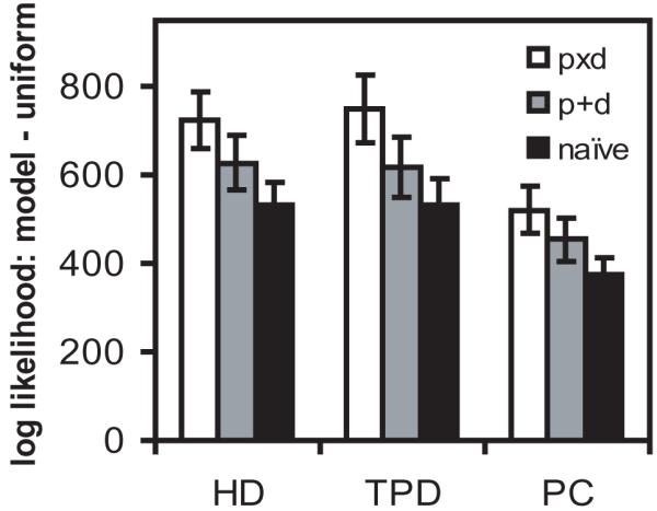
The relative goodness of fit of naïve, additive (p+d) and factorial (pxd) models of the locational and directional influences on the firing rate of place cells (PC) head-direction cells (HD) and theta-modulated place-by-direction cells (TPD). The difference in the log likelihood of the data under the given model and under a uniform firing rate model is shown. For example, for the factorial model l_×-l_u is shown, see text. The naïve model is based on the traditional separate histograms of firing rate by location and direction. A square grid of location bins was used such that on average 68 bins were occupied (i.e. mean N_l = 68, this smaller number cf. Figures 1-3 was used to aid convergence of equation 7 for the additive model) and 64 direction bins were used (i.e. N_d = 64). The mean and s.e.m. are shown for the 29/46 PC, 30/46 HD and 33/46 TPD cells for which equation 7 converged. The differences between the bar heights for each model is significant for each cell type (p<10^-6, paired sample t-test). The ‘simple normalisation’ approach to estimating p_i and d_j (see text) showed a worse overall fit than any of the above models, with l_s-l_u = 346 for PCs, 485 for HDs and 465 for TPDs when l_s is found using λ_ij = ½(p_i + d_j)t_ij in equation 5, and 414 for PCs, 450 for HDs and 55.4 for TPDs when l_s is found using λ_ij = p_i d_j t_ij.

Finally a ‘simple normalisation’ approach would be to take the locational firing rate as the mean firing rate over all directions sampled at that location (to remove dependence on the time spent in each direction), and similarly the directional firing rate as the mean firing rate over all locations sampled at that direction i.e.: p_i = Σ_j (n_ij/t_ij) / N_d, and d_j = Σ_i (n_ij/t_ij) / N_l. However, the sampling of positions and directions in typical data is so sparse that the means are dominated by extreme rates from very short duration samples (while the medians are zero), so that this approach fares worse than the naïve model, see Figure 5 caption.

The goodness of fit of different models can be assessed by comparing the log likelihood (l) of the data under each model. We do this using equation 5, under the assumption of Poisson noise, calculating: l_× with λ_ij = p_i d_j t_ij from equation 6 for the factorial model; l₊ with λ_ij = (p_i+d_j)t_ij from equation 7 for the additive model; l_n with λ_ij = ½(n_i/t_i+n_j/t_j)t_ij for the naive model; and l_u with λ_ij = (Σ_ij n_ij / Σ_ij t_ij)t_ij for the prediction of a uniform firing rate model. The goodness of fit of the naïve, additive and factorial models to place, head-direction and TPD cell firing is shown in Figure 5 (as log scores of the factor by which the data are more likely under a given model than under the uniform model, e.g. l_×-l_u). There is a clear advantage for the factorial model over the available alternatives. Although this does not conclusively rule out an additive model, since our estimate is not necessarily the additive model that maximizes the likelihood of the data, factorial rather than additive models are consistent with the very low firing rates of TPD cells outside of their preferred location and direction (and with the low firing rate of place cells outside the place field, despite its modulation by running speed, McNaughton, Barnes, & O’Keefe, 1983; Wiener, Paul, & Eichenbaum, 1989; Huxter, Burgess, & O’ Keefe, 2003). Data may also contain more complex dependencies that are not well characterized by any of these models (e.g. two locational subfields with different preferred directions). Such data can sometimes be divided so that each subset of observations is well fitted. In this case, the (geometric) mean likelihood per observation in a subset of N observations (exp(l/N)) can be used to indicate whether the division was justified or not.

In conclusion, we believe that our approach for separating the influences of multiple independent causes made dependent by inhomogeneous sampling, or an equivalent approach, is required before correct assessment can be made of the contribution of any one variable where there is a contribution from a second variable. This approach is related to the converse problem of how a factorial code can enable multiple cells to encode a single variable (see e.g. Schneidman, Bialek, & Berry, 2003; Schmidhuber, 1992). We have illustrated the application of our approach to place and direction correlates of cell firing in single units recorded in freely moving rats. A spurious impression of positional or directional correlates created by inhomogeneous sampling of places and directions is commonplace when using the traditional method of separately forming histograms of numbers of spikes divided by dwell-times. The use of an explicit maximum-likelihood factorial model of the independent influences of position and orientation succeeds in reducing the problems posed by inhomogeneous sampling, and provides an improvement on the available alternatives (the standard separate histograms or an additive model). This opens the way to assess the firing patterns of cells for which both variables have an effect (e.g. Figure 3), and to assess the contribution of one variable under manipulations of the other (e.g. Figure 4). In principle our method could be used to disentangle the combined effects of behavioral variables other than location and orientation (e.g. running speed) so long as there is a well-defined metric for the values observed.