Spatial and seasonal patterns in climate change, temperatures, and precipitation across the United States

Abstract

Changes in climate during the 20th century differ from region to region across the United States. We provide strong evidence that spatial variations in US temperature trends are linked to the hydrologic cycle, and we also present unique information on the seasonal and latitudinal structure of the linkage. We show that there is a statistically significant inverse relationship between trends in daily temperature and average daily precipitation across regions. This linkage is most pronounced in the southern United States (30–40°N) during the May-June time period and, to a lesser extent, in the northern United States (40–50°N) during the July-August time period. It is strongest in trends in maximum temperatures (T_max) and 90th percentile exceedance trends (90PET), and less pronounced in the T_max 10PET and the corresponding T_min statistics, and it is robust to changes in analysis period. Although previous studies suggest that areas of increased precipitation may have reduced trends in temperature compared with drier regions, a change in sign from positive to negative trends suggests some additional cause. We show that trends in precipitation may account for some, but not likely all, of the cause point to evidence that shows that dynamical patterns (El Niño/Southern Oscillation, North Atlantic Oscillation, etc.) cannot account for the observed effects during May-June. We speculate that changing aerosols, perhaps related to vegetation changes, and increased strength of the aerosol direct and indirect effect may play a role in the observed linkages between these indices of temperature change and the hydrologic cycle.

The rate of warming and changes in other climate variables such as sea-level rise vary over the globe. For arriving at reliable predictions of future changes it is important both to characterize regional climate change differences and to understand the underlying climate processes. In this article, we focus on the observed spatial variations of trends in daily maximum temperature and its extremes (e.g., trends in the hottest or coolest 10% of daily maxima) along with related climate change indices such as trends in daily minimum temperatures, using records of daily temperatures for 1950–2006 at stations across the continental United States. Sharp contrasts in the nature of the changes in daily maximum and minimum temperature are identified, with certain regions displaying trends toward substantial increases in daily maximum temperatures, in particular, whereas others display much smaller warming trends or even trends toward cooler values. We show that the largest warming trends of daily maximum temperature have occurred in dry locations, whereas wetter regions have been subject to negative trends. Further, changes in the hottest 10% of daily maxima display the strongest dependence on precipitation and the strongest seasonality, in particular, in the months of May and June from 30° to 40°N and to a lesser extent in July and August from 40° to 50°N.

A number of papers have probed the relationship between temperatures, clouds, and precipitation (e.g., refs. 1–3). Note that in this article we only use precipitation, but because clouds and precipitation are strongly correlated we implicitly include much of the cloudiness signal. Ref. 1 extensively probed the connection between precipitation and T_max and diurnal temperature range (DTR), showing strong anticorrelation of precipitation, T_max, and DTR on short timescales (up to interannual) during the warm season. These are caused primarily by reductions of solar heating by clouds and increases in surface latent heat release by surface wetness increases due to precipitation. They suggest that long-term changes in precipitation and clouds may be the cause of reduced temperature trends and negative DTR trends. We explore this in detail below. Recently, it has been shown that trends in temperature and DTR show a strong dependence on precipitation amount on a global scale (4). We carry out a similar but more detailed analysis on the continental United States and expand the analysis to include seasonality and effects on the extremes in the distribution. Differences with ref. 4 are noted below.

The southeastern United States is one of the few places in the world displaying an overall cooling trend over the 20th century, in contrast to the widespread global warming (5). A number of articles have explored this anomaly (6–9). Note that several of these find the anomalous region in the central United States and not in the Southeast depending on the time interval and the dataset used (we show below that it is most prominent in the early summer in the southeastern United States and in the late summer in the north-central United States). It is not clear whether a common explanation is possible for both the southeastern and central United States. No consensus exists to adequately explain these anomalous regions. For example, one study used a global climate model forced by observed sea surface temperatures (SSTs) to suggest that SSTs can force the anomaly in the east-central United States (6). Others used downscaling in regional models and proposed different mechanisms that can simulate the “warming hole” [a circulation/soil moisture feedback (7) and better cumulus parameterization (8)]. Another suggested that internal dynamic variability could be the cause of the anomaly in the central United States by analyzing multiple simulations from 18 climate models (9). In addition, large-scale circulation modes [El Niño/Southern Oscillation (ENSO), Arctic Oscillation, etc.] may play a role and are discussed more below. The lack of consensus in these articles is a key motivation for further characterization of the observations as provided in this article, to obtain constraints to test various theories. In this article we probe relationships between precipitation (both climatological and trends) and trends in both maximum and minimum temperatures, and trends in their extremes and the seasonal and latitudinal patterns of the correlations. The finding that the anomalous negative trends in daily temperature maxima in the Southeast over the past 50 years appear to be most closely tied to hydrologic parameters, and elucidation of its seasonal cycle, is of particular interest for attempts to explain the unusual changes observed in the climate of this region. We propose speculative mechanisms to explain the observed connections between daily maximum temperatures and precipitation below.

Results

The Global Historical Climatology Network Daily (GHCND) station data (Version 1) that are used in this study provide daily minimum and maximum temperatures and precipitation amounts at thousands of stations in the United States (10). We concentrate on the years 1950–2006 because there are a large amount of data present throughout the continental United States over this time interval and several studies have focused on this time interval (e.g., ref. 11). However, as discussed below, our results are robust to changes in time interval. We include all stations with >50 years of data throughout this period. The mean precipitation, trend in T_min, T_max, and T_mean, and trends in percent exceedance of percentiles (e.g., 10, 50, and 90%) are computed at each station. In general, we have used a 90% available data threshold to include data in the analysis. This threshold is applied in a given time period (e.g., a 2-month period to compute a mean) and when computing a trend (90% of the years must have averages). The computation of the trends of percentile exceedance is discussed below.

Temperature Trends, and Precipitation.

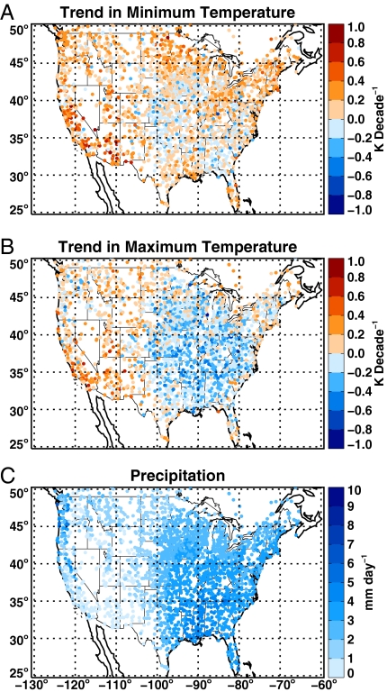
We computed trends in temperature monthly, bimonthly, and seasonally. We present examples here for the May-June period first because this period has the highest degree of statistical significance for the linkage we are exploring (this is discussed further below). Fig. 1 A and B shows maps of trends in daily minimum and maximum temperature for all US GHCND stations with data in the 1950–2006 time interval satisfying the criteria discussed above. Fig. 1C shows the average precipitation for the March-June period for the same stations (the addition of earlier months is discussed below). The map of trends in maximum temperature (Fig. 1B) shows a large variation across the United States in going from east to west, and smaller variations north to south, whereas the minimum temperature map (Fig. 1A) is more homogeneous. The large area of negative trends in the southeastern United States is in the same general region as the negative 20th century temperature trends for this time period (5). Fig. 1 shows that this Southeast anomaly region of trends in maximum temperature is characterized by a high precipitation rate. It is striking that the 100th meridian, which provides a demarcation for the transition between the drier western and wetter eastern United States (sometimes referred to as the “dry line,” see Fig. 3 below), separates the regions of negative and positive trends in Fig. 1B.

Fig. 1.

Maps of 1950–2006. (A) Minimum temperature trends for May-June, (B) same as A but for the maximum temperature, and (C) mean daily precipitation (mm/day) but for March-June time period (earlier months included because effects of precipitation may persist for several months; see Discussion). All stations are shown that satisfy minimum data requirements discussed in the text.

Fig. 3.

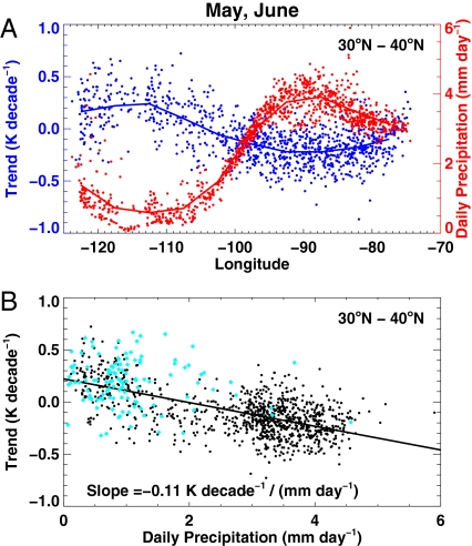
1950–2006 May-June daily maximum temperature trends together with March-June average daily precipitation for 30–40°N. (A) Longitudinal variation. Solid lines show the averaged results and the points show individual stations. (B) Scatter plot of the points in A along with a least-squares trend line fitting the data. The points in the region 115–125°W and 30–40°N (primarily California) are highlighted in cyan.

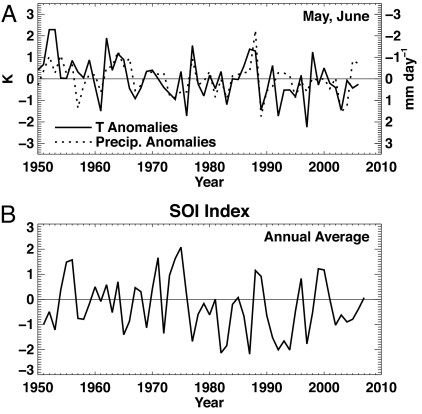
The average T_max anomaly time series is shown in Fig. 2 for a region of the southeastern United States (80–95°W, 30–40°N) along with the average precipitation and the Southern Oscillation Index (SOI) (from http://www.cpc.ncep.noaa.gov/data/indices). The anomaly is computed by removing the long-term mean temperature at each station and averaging all stations in the region. The anomalies of mean precipitation have been overlaid on Fig. 2 Upper (dashed line) with scale reversed, clearly demonstrating the large degree of anticorrelation between these variables (r = −0.57), as noted by previous studies (1, 3). The anticorrelation likely comes from both the surface wetness effects of precipitation and the effects of clouds associated with the precipitation discussed above. However, correlation on shorter timescales does not necessarily imply strong links in longer-term trends. To account for both the annual and long-term changes in the precipitation time series on the temperature time series to first order, we compute the trend of the temperature time series with and without including the precipitation time series as a linear regression term. The trend in temperature changes from −0.21 to −0.14 K decade⁻¹ demonstrating a role for trends in precipitation but for only a small amount of the anomalous trend. We revisit this using a larger geographic scale below. The DTR time series shows even larger annual correlation with average precipitation (r = −0.78), but the long-term trend is similarly little affected. Even less connection of the SOI index and the temperature time series is evident (r = 0.03).

Fig. 2.

Time series of annually averaged daily maximum temperature and mean precipitation anomalies for a region of the southeastern United States (80–95°W, 30–40°N) (A) and the SOI (B). Note the reversed scale used for the average precipitation anomalies on A that demonstrate the large short-term anticorrelation (r = −0.57).

To further explore the relationship between trends in daily maximum temperature and the mean precipitation, a longitudinal cross-section of stations located from 30–40°N latitude is shown in Fig. 3A. This figure indicates that the large change in mean precipitation that occurs near 100°W longitude coincides with a distinct change in the temperature trend. Significantly, the relationship to precipitation is not restricted to the large-scale change seen in crossing the dry line: smaller changes in the temperature trend (for example, stations in the Northwest and in California) are also colocated with consistent changes in precipitation (see also, Fig. 3B).

A scatter plot of all observations in Fig. 3A is shown in Fig. 3B along with a trend line fitting the data. Fig. 3B demonstrates and quantifies the relationship between these variables, which can be visually observed in Figs. 1 and 3A. The cyan subset of points in Fig. 3B represents stations from 115–125°W, and from 30–40°N (primarily in California), illustrating that the relationship of trends in maximum temperature to precipitation occurs to some degree across that region and in the larger scale. Estimating the degree of significance of the slope of the mean precipitation versus temperature trend scatter plot is complicated by the large amount of spatial correlation among nearby stations in particular years, both in the average precipitation and temperature trend fields. If unaccounted for, this correlation would artificially inflate the significance of the relationship because of an overestimation of the number of independent points. To account for this correlation and estimate the 1 and 2 sigma slopes about the null hypothesis (zero slope, i.e., no connection between the trend in daily maximum temperature and climatological precipitation) the observational temperature and precipitation time series are used, but the ordering of the years is randomized. The same randomization of years is used for all stations to preserve the spatial correlations. The precipitation versus temperature trend slope is recomputed for the randomized data and this procedure is repeated 10,000 times to obtain a distribution of slopes, from which the 1 and 2 sigma values are obtained for the null hypothesis that there is no time dependence in the relationship between climatologically average precipitation and temperature anomalies. The 2-sigma estimate for the slope on Fig. 3B is 0.04 (K decade⁻¹)/(mm day⁻¹), demonstrating that the computed slope of −0.11 (days decade⁻¹)/(mm day⁻¹) is highly significant.

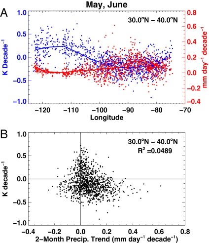
To explore the possibility that precipitation trends might have caused the reduction of the temperature trends in the southeastern United States, we show the longitudinal variation of precipitation trend and the temperature trend on Fig. 4A. A small increase in the precipitation trend is evident in the southeastern United States, but it is relatively small compared with the variability and not well correlated with trends in maximum temperature. Fig. 4B shows a scatter plot of the data in Fig. 4A. It is evident that there is no significant relationship between these variables above the variability across the Southern United states. Using % decade⁻¹ instead of mm decade⁻¹ (to enhance the trends in dry regions) does not improve the relationship (data not shown). The nearly complete lack of any relationship between these variables is strong evidence that trends in precipitation are not the cause of negative trends in T_max in the southeastern United States.

Fig. 4.

1950–2006 May-June daily maximum temperature trends together with average daily precipitation trends for 30–40°N. Like Fig. 3, except that precipitation trend is used in place of mean precipitation. The least-squares fit line is not shown on B because the relationship between these variable is weak compared with the variability.

Percentile Exceedance Trends and Precipitation.

We have demonstrated that there is a large difference between trends in minimum and maximum temperature in the southeastern United States. We now explore whether this change also affects different parts of the daily temperature distribution differently, and how changes in temperature extremes relate to precipitation. We will use trends in percentile exceedance in the tails of the distributions to quantify the trends of extreme values (11, 12). The trend in exceedance rate of percentiles is computed in the following way. First, at each station the percentiles on each day of the year are computed by using all temperatures within a 5-day window about that day for all years with data. The 5-day window is used to improve the statistics of the percentile calculation. In this article, we use the term “time interval” to refer to the entire time history used (e.g., 1950–2006) and “time period” to refer to the period in the year that statistics are combined (e.g., May-June). A time period in a given year is only included if 90% of the data are present. Data are used, on a given day-of-year, only if 90% of the data within the 5-day window is available over the entire time interval. Next, we compute the exceedance rate for days that exceed the 90^th percentile including all days within the desired time period. Finally, the least-squares trend of the exceedance rate time series is computed if 90% of the years have exceedance rates present, and it is converted to days/decade by multiplying by the number of days in that time period (assuming no missing data). We label the 90th percentile exceedance trend 90PET.* We use the same time interval for the percentile computation and the trend calculation and thus avoid inhomogeneities in the exceedance time series that other methods can produce (14). Note that the pattern of changes in 90PET found with GHCND stations is very similar to that seen if a sparser, tightly quality controlled network of stations is used [Expert Team on Climate Change Detection and Indices (ETCCDI); see ref. 11].

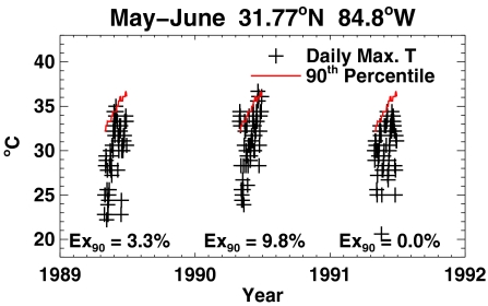
Fig. 5 illustrates the method using daily temperatures at one GHCND station. Three years of data are shown. The daily percentile values have been computed over the entire 1950–2006 time interval. The exceedances in each of the 3 years are readily seen, and the percentage of data exceeding the 90th percentile in each year is indicated on the graph; these are the basis for computation of the trends in exceedance rates.

Fig. 5.

Illustration of typical observations and the method of computing exceedance rates. The red line shows the 90th percentile values of daily maximum temperature for the selected station (Cuthbert, GA, GHCND ID 42500092450) over the time interval (1950–2006) for May and June. Crosses represent observations in 1989, 1990, and 1991, showing those days when exceedances of the 90th percentile of T_max are observed. The averaged exceedance rates for May-June in each year (Ex₉₀) are indicated.

The trend in the exceedance rate is an interesting quantity for several reasons. It is intuitive, because it is easier to relate to a trend in days/decade than one in K/decade. It also accounts for the seasonal cycle by using the percentile values on each day. It is sensitive to relatively small changes in extremes, but this can also cause the trend values of exceedance to saturate if the trends in temperature are too large. For example, if there is a large positive trend then it is possible for the early portions of the time series to have no exceedances and the later portions to have 100% exceedances. This would cause the exceedance trend to be saturated. For the US stations used in this study, the exceedance trends are not saturated and are a useful and sensitive way to examine trends in the tails of the temperature distribution. One could also analyze trends in the tails of the temperature time series by computing the trend of the 90th percentile values directly by using all of the points in each time period of every year (e.g., ref. 15) or by analyzing changes in absolute extremes, such as the warmest day in a year. The direct percentile approach avoids the saturation problem but has the disadvantage of computing the percentiles with a combination of seasonal cycle and daily variability, which only captures changes in the peak warm/cold season and may have poorer sampling properties.

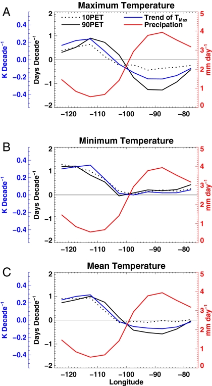
We show the 10 and 90PET for daily maximum and minimum temperatures on Fig. 6 A and B as a function of latitude, along with the trends in mean daily minimum and maximum temperature already presented. The trends for both the high and low side of the temperature distribution (10 and 90PET) are contrasted with the overall trend in temperature. The maximum temperature shows a distinct difference between the 10 and 90PET fields in the southeastern United States, with much larger negative trends observed in 90PET. The trend in mean daily maximum temperature displays characteristics of both 10 and 90PET, with closer similarity to 90PET, indicating a distinct shift in the temperature distribution toward a shorter upper tail. The minimum temperature distribution shows much less variation between the trend in the mean, upper tail, and lower tail of the distribution (trend, 90PET, and 10PET, respectively) and the shape of the changes is much less similar to that of mean precipitation. It is interesting to note that the maximum temperature 10PET curve is similar to the minimum temperature statistics, although the 10PET of daily maximum temperature shows small negative trends compared with small positive trends of the daily minimum temperature in the southeastern United States. Fig. 6C shows how the anomalous behavior observed in the maximum temperature fields affects the mean temperatures, i.e., the quantity most often used in climate studies. Overall this figure shows that much of the changes in the extremes are driven by a shift in the entire distribution of temperatures. This is especially true for the daily minimum temperatures. The daily maximum temperatures show evidence for enhanced changes in the high side of the distribution. As illustrated in Fig. 6A the 90PET field is even more strongly related to the mean precipitation than the overall trend in temperature and so we will now focus on it.

Fig. 6.

Variation of the 1950–2006 average precipitation, the 10th and 90th percentile exceedance trends (10 and 90PET, exceedance toward higher temperature extremes), and the trend in temperature as a function of longitude for all stations 30–40°N. The temperature statistics are for the May-June period and precipitation for the March-June period. Stations have been averaged into 5° longitude bins. Maximum, minimum, and mean temperature statistics are shown in A–C, respectively.

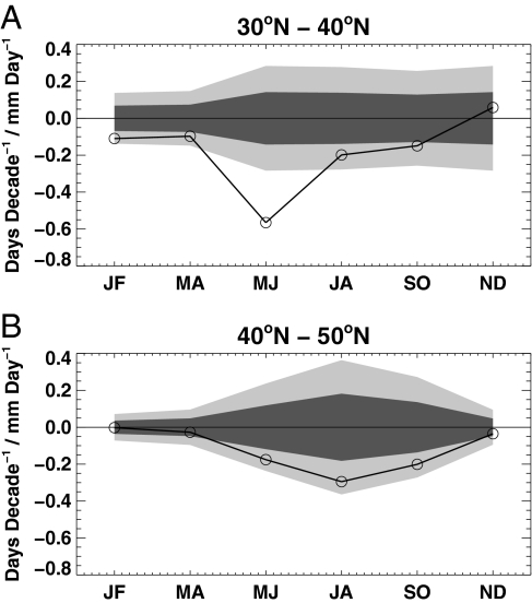
The seasonal variation of the correlation slope of the precipitation-90PET relationship is shown in Fig. 7, along with the 1- and 2-sigma confidence intervals computed as described above. Data for 30–40°N and 40–50°N latitude regions are shown separately to probe latitudinal changes. The slope is negative and significant at least to the 1-sigma level throughout the year except in November-December in the 30–40°N region. The May-June time period shows a very strong correlation that is significant at well beyond the 2-sigma level, as noted above. A similar analysis using monthly time periods shows that the May and June months individually show the most significant correlation of all months. When computed seasonally, both the March-April-May and June-July-August time periods show significant correlations, in large part from the strong effect of May and June individually. Thus, we chose to show the May-June combined period in Figs. 1– for the 30–40°N region. The 40–50°N region shows a similar seasonality, but the most negative slope is found for this region in the July-August time period, and the correlation becomes small and statistically insignificant for the months November through April. However, both the May-June and July-August periods are significant at near the 2-sigma level for 40–50°N. The delay of the large negative slopes as one goes northward may provide clues in understanding the causes of this effect, as discussed below.

Fig. 7.

Slope of the relationship between the daily maximum temperature 90th percentile exceedance trends (90PET) and the daily mean precipitation for 30–40°N (A) and 40–50°N (B) versus time (2-month intervals labeled by leading initials of the months). One- and 2-sigma confidence intervals based on the approach outlined in the text are indicated by the dark and light shading, respectively.

Discussion

The results shown in this article clearly demonstrate a connection in the southern United States (30–40°N) between the regional changes in daily maximum temperatures, in particular, the overall trend and the 90th percentile exceedance trends (90PET) and climatological mean precipitation through much of the year, but most strongly in the May-June time period. In contrast, this relationship is absent in November and December in the southern United States, and between November and April in the northern United States (40–50°N). This connection between precipitation and changes in the number of warm days is quite robust. It is noteworthy that the relationship is much weaker for daily minimum (i.e., nighttime) temperatures, and for the 10PET of daily maximum temperatures, so this behavior is most strongly a property of the middle and high part of the daily maximum temperature distribution. We obtain similar results when using precipitation frequency in place of mean precipitation.

We have probed the effect of including mean precipitation for months previous to the time period used in the 90PET calculation in examining these relationships. We find that including 2 months previous in the precipitation calculation improves the statistical significance of the precipitation-90PET connection. However, using the mean for the same months as the 90PET calculation, including only the month before, or using the mean precipitation for the entire year all give qualitatively the same result. The large temperatures present in the 1950s (see Fig. 2) raise concern that the observed relationship is sensitive to the time interval used. We have computed the exceedance–precipitation relationship for May-June using time intervals starting in 1900, 1940, 1960, 1970 (all ending in 2006) and in all cases the result is qualitatively the same, although the trends are somewhat smaller when using 1900 or 1970 as the starting point.

Note that the relationship between hydrological parameters and daily maximum temperatures has been probed here specifically for the United States, and does not appear to be universal across the globe. Although a detailed analysis of all other regions is beyond the scope of the present study, we note, for example, that trends over the past 50 years based on ETCCDI indices (11) show increases in the number of hot daily maxima over large parts of China that are quite distinct in their relationship to precipitation from that shown here for the United States (including, e.g., the climatologically wettest easterly coastal region, whereas decreases can be seen in the Beijing area and southwest of it, and in the Southwest corner of China, which are climatologically drier). It was recently found that trends in daily maximum and minimum temperature decrease with increasing precipitation when a nearly global dataset is used (4), but several differences exist between these authors' result and ours. First, they find no precipitation amount that gives negative trends, only smaller positive trends. Second, they find a stronger relationship with T_min and their DTR trend is found to increase with increasing precipitation, whereas in the southern United States we find a stronger relationship with T_max and decreasing DTR trends with increasing precipitation in May-June and no significant DTR variation with precipitation in the annual average. Our study complements that in ref. 4 by focusing on an anomalous region, by exploring extremes (which tighten the relationships), and by showing the seasonality and spatial changes of the relationship.

The primary purpose in this article is to present the correlations between daily minimum and maximum temperature changes, temperature extremes, and precipitation across the United States. Although this study does not focus on the cause of this relationship, it is reasonable to consider possible connections between these properties. As noted in the introduction, previous explanations for this (or a similar) phenomenon include: trends in precipitation (e.g., ref. 1), effects of SSTs (6), local microclimatic effects (7, 8), and internal variability of the climate system (9). We show above that trends in precipitation are not able to explain the spatial patterns observed (Figs. 2 and 4). The effects of SSTs and the downscaling results were confined to the central United States and not the southeastern United States. It is unclear whether a similar phenomenon could operate in the southeastern United States. Large-scale modes of climate variability (ENSO or interdecadal Pacific variability) can cause a pattern of cooling in the southeastern United States (see, for example, refs. 16 and 17) but the response is primarily in the winter season and affects the upper tails of both minimum and maximum temperature (17). The response of ENSO in the summer (May-October) is small in the southeastern United States (figure 4 of ref. 17) and when that analysis is restricted to May-June it is still found to be small, even if appropriate lags in the response to ENSO are considered (this is true of the other modes studied as well). Also, the poor correlation between changes in daily maximum temperature and the SOI (Fig. 2) does not support a link to ENSO. Climate variability could certainly be playing a role but it should be noted that ref. 9 finds cooling in the central United States in summer and not the southeastern United States, and statistically significant relationships between trends in maximum temperature and the mean precipitation that do not depend on trend length would be difficult to explain by internal climate variability.

Precipitation and cloudiness are strongly correlated and thus the relationships we find could be related to either. Both clouds and precipitation are expected to damp local greenhouse warming; clouds, although a direct reduction of the anthropogenic greenhouse effect, and precipitation, by increasing surface wetness and thus increasing evaporation at the expense of sensible heating. This is likely the cause for much of the decrease of trends in daily maximum temperature we have found (and those found globally in ref. 4) but one would not expect either of these effects to produce negative trends in temperature. A number of speculative possibilities exist for producing even larger reductions in the trend, resulting in the negative trends observed in this article.

The southeastern United States is known to be cloudy and with a high population density it is likely a rich source of aerosol from the many cities and towns. Thus, an enhanced direct and indirect effect could be responsible. However, it is unclear why this effect alone would produce the seasonality found in Fig. 7. Furthermore, other cloudy regions with large amounts of industrial activity do not show this behavior. Something more uniquely tied to this region appears to be necessary. The strong seasonality of the trend and its delay as one moves northward suggest a possible link to the growing season. The southeastern United States has a large source of volatile organic molecules; concentrations of gases such as isoprene in the southeastern United States are comparable to those obtained in the Amazon (18). Recent measurements show that a large fraction of the secondary organic aerosol (SOA) in this region is of biogenic origin (e.g., ref. 19) and that SOA of biogenetic origin may have higher yields in regions with elevated anthropogenic pollution (20). The wet Southeast has also experienced an extensive revegetation of the natural forest after clearing for agriculture in the late 18th and early 19th centuries (21). Although clearly speculative, increasing biogenic secondary organic aerosol/cloud effects linked to forest regrowth and/or interactions with anthropogenic pollution is one possibility that is qualitatively consistent, not only with the spatial structure, but also with the seasonality of the correlation of the unusual negative temperature trends with precipitation found in the southeastern United States. Detailed process-based modeling studies would be required to proof this hypothesized relationship, which is beyond the scope of the present article.

Whatever its cause, we find the highly significant negative relationship between precipitation and trends in maximum temperature and its extremes to be intriguing, and it strongly suggests a link between some type of hydrologic process and key aspects of the pattern of climate trends across the United States.

Materials and Methods

The GHCND temperature and precipitation data were obtained from ftp://ftp.ncdc.noaa.gov/pub/data/ghcn/daily and the SOI was obtained from http://www.cpc.ncep.noaa.gov/data/indices.

References

- 1.Dai A, Trenberth KE, Karl TR. Effects of clouds, soil moisture, precipitation, and water vapor on diurnal temperature range. J Climate. 1999;12:2451–2473. [Google Scholar]
- 2.Madden RA, Williams J. The correlation between temperature and precipitation in the United States and Europe. Monthly Weather Rev. 1978;106:142–147. [Google Scholar]
- 3.Trenberth KE, Shea DJ. Relationships between precipitation and surface temperature. Geophys Res Lett. 2005 doi: 10.1029/2005GL022760. [DOI] [Google Scholar]
- 4.Zhou L, et al. Spatial dependence of diurnal temperature range trends on precipitation from 1950 to 2004. Clim Dyn. 2008 doi: 10.1007/s00382-008-0387-5. [DOI] [Google Scholar]
- 5.Trenberth KE, et al. Observations: Surface and atmospheric climate change. Climate Change 2007: The Physical Science Basis. In: Solomon S, et al., editors. Contribution of Working Group I to the Fourth Assessment Report of the Intergovernmental Panel on Climate Change. Cambridge, UK: Cambridge Univ Press; 2007. pp. 235–336. [Google Scholar]
- 6.Robinson WA, Reudy R, Hansen JE. General circulation model simulations of recent cooling in the east-central United States. J Geophys Res. 2002 doi: 10.1029/2001JD001577. [DOI] [Google Scholar]
- 7.Pan Z, et al. Altered hydrologic feedback in a warming climate introduces a “warming hole.”. Geophys Res Lett. 2004 doi: 10.1029/2004GL020528. [DOI] [Google Scholar]
- 8.Liang XZ, et al. Regional climate model downscaling of the U.S. summer climate and future change. J Geophys Res. 2006 doi: 10.1029/2005JD006685. [DOI] [Google Scholar]
- 9.Kunkel KE, Liang XZ, Zhu J, Lin Y. Can CGCMs simulate the twentieth-century “warming hole” in the central United States. J Climate. 2006;19:4137–4153. [Google Scholar]
- 10.Vose R, Menne M, Durre I, Gleason B. GHCN-Daily: A global dataset for climate extremes research. EOS Trans AGU. 2007;88:A41A–08. Jt Assem Suppl. (abstr) [Google Scholar]
- 11.Alexander LV, et al. Global observed changes in daily climate extremes of temperature and precipitation. J Geophys Res. 2006 doi: 10.1029/2005JD006290. [DOI] [Google Scholar]
- 12.Easterling DR, et al. Climate extremes: Observations, modeling, and impacts. Science. 2000;289:2068–2074. doi: 10.1126/science.289.5487.2068. [DOI] [PubMed] [Google Scholar]
- 13.Frich P, et al. Observed coherent changes in climatic extremes during the second half of the twentieth century. Climate Res. 2002;19:193–212. [Google Scholar]
- 14.Zhang XB, Hegerl G, Zwiers FW, Kenyon J. Avoiding inhomogeneity in percentile-based indices of temperature extremes. J Climate. 2005;18:1641–1651. [Google Scholar]
- 15.Robeson SM. Trends in time-varying percentiles of daily minimum and maximum temperature over North America. Geophys Res Lett. 2004 doi: 10.1029/2003GL019019. [DOI] [Google Scholar]
- 16.Ropelewski CF, Halpert MS. North American precipitation and temperature patterns associated with the El Nino/Southern Oscillation (ENSO) Monthly Weather Rev. 1986;114:2352–2362. [Google Scholar]
- 17.Kenyon J, Hegerl GC. Influence of modes of climate variability on global temperature extremes. J. Climate. 2008 doi: 10.1175/2008JCLI2125.1. [DOI] [Google Scholar]
- 18.Greenberg JP, et al. Tethered balloon measurements of biogenic VOCs in the atmospheric boundary layer. Atmos Environ. 1999;33:855–867. [Google Scholar]
- 19.Lewis CW, Klouda GA, Ellenson WD. Radiocarbon measurement of the biogenic contribution to summertime PM-2.5 ambient aerosol in Nashville, TN. Atmos Environ. 2004;38:6053–6061. [Google Scholar]
- 20.Weber RJ, et al. A study of secondary organic aerosol formation in the anthropogenic-influenced southeastern United States. J Geophys Res. 2007 doi: 10.1029/2007JD008404. [DOI] [Google Scholar]
- 21.Hurtt GC, et al. The underpinnings of land-use history: Three centuries of global gridded land-use transitions, wood-harvest activity, and resulting secondary lands. Global Change Biol. 2006;12:1208–1229. [Google Scholar]