

Abstract
Indicator kriging provides a flexible interpolation approach that is well suited for datasets where: 1) many observations are below the detection limit, 2) the histogram is strongly skewed, or 3) specific classes of attribute values are better connected in space than others (e.g. low pollutant concentrations). To apply indicator kriging at its full potential requires, however, the tedious inference and modeling of multiple indicator semivariograms, as well as the post-processing of the results to retrieve attribute estimates and associated measures of uncertainty. This paper presents a computer code that performs automatically the following tasks: selection of thresholds for binary coding of continuous data, computation and modeling of indicator semivariograms, modeling of probability distributions at unmonitored locations (regular or irregular grids), and estimation of the mean and variance of these distributions. The program also offers tools for quantifying the goodness of the model of uncertainty within a cross-validation and jack-knife frameworks. The different functionalities are illustrated using heavy metal concentrations from the well-known soil Jura dataset. A sensitivity analysis demonstrates the benefit of using more thresholds when indicator kriging is implemented with a linear interpolation model, in particular for variables with positively skewed histograms.
Keywords: interpolation, thresholds, cross-validation, jack-knife, accuracy, Fortran
1. Introduction
Two common features of environmental datasets are the occurrence of a few very large concentrations (hot-spots) and the presence of data below the detection limit (censored observations). Extreme values can strongly affect the characterization of spatial patterns, and subsequently the prediction. Several approaches exist to handle strongly positively skewed histograms (Saito and Goovaerts, 2000). One common approach is to first transform the data (e.g. normal score, Box Cox or lognormal transform), perform the analysis in the transformed space, and back-transform the resulting estimates. Such transform, however, does not solve problems created by the presence of numerous censored data since either it yields a spike of similar transformed values or, in the case of the normal-score transform, it requires a necessarily subjective ordering of all equally-valued observations. Moreover, except for the normal score transform (Deutsch and Journel, 1998), it does not guarantee the normality of the transformed histogram, which is required to compute confidence intervals for the estimates. Last, the back-transform of estimated moments is not straightforward and can introduce bias if not done properly (Saito and Goovaerts, 2000); for example, lognormal kriging estimates cannot simply be exponentiated. Another way to attenuate the impact of extreme values is to use more robust statistics and estimators. The non-parametric approach of indicator kriging (IK) falls within that category (Journel, 1983; Goovaerts, 2001). The basic idea is to discretize the range of variation of the environmental attribute by a set of thresholds (e.g. deciles of sample histogram, detection limit, regulatory threshold) and to transform each observation into a vector of indicators of non-exceedence of each threshold. Kriging is then applied to the set of indicators and estimated values are assembled to form a conditional cumulative distribution function (ccdf). The mean or median of the probability distribution can be used as an estimate of the pollutant concentration (e.g. Barabas et al., 2001; Cattle et al., 2002; Goovaerts et al., 2005).
A frequent criticism of the indicator approach is that the binary coding amounts to discarding some of the information in the data. In theory, this loss of information can be compensated by accounting for indicator values defined at different thresholds, that is using indicator cokriging instead of kriging. Practice has shown, however, that indicator cokriging improves little over indicator kriging (Goovaerts, 1994; Pardo-Igúzquiza and Dowd, 2005) because cumulative indicator data carry substantial information from one threshold to the next one, and all indicator values are available at each sampled location (isotopic or equally-sampled case). Another way to increase the resolution of the discrete ccdf is to conduct a fine discretization of the continuous sample distribution using a large number of thresholds. For example, 15 indicator cutoffs were used by Lark and Fergusson (2004) to map the risk of soil nutrient deficiency in a field of Nebraska. Goovaerts et al. (2005) used indicator kriging with 22 thresholds to model probabilistically the spatial distribution of arsenic concentrations in groundwater of Southeast Michigan. Cattle et al. (2002) used 100 threshold values to characterize the spatial distribution of urban soil lead contamination. The extreme situation is to identify the set of thresholds with the sample dataset, that is to use as many thresholds as observations. In this case, typically only the observations the closest to the interpolated location (e.g. located within the search window) are used as thresholds. Such tailoring of thresholds to the local information available leads to a better resolution of the discrete ccdf by selecting low thresholds in the low-valued parts of the study area and high thresholds in the high-valued parts (Saito and Goovaerts, 2000; Lloyd and Atkinson, 2001; Cattle et al., 2002).
The trade-off costs for the finer resolution of the ccdf are the tedious inference and modeling of multiple indicator semivariograms, as well as the increasing likelihood that the estimated probabilities won’t honor the axioms of a cumulative distribution function: all probabilities must be valued between 0 and 1 and form a non-decreasing function of the threshold value. Failure to honor such constraints, referred to as order relation deviations, requires the a posteriori correction of the set of estimated probabilities (Deutsch and Journel, 1998). To keep these deviations within reasonable limits, Deutsch and Lewis (1992) recommend using no more than 9–15 thresholds. Several authors have proposed alternate implementations of the indicator approach that reduce the proportion and magnitude of order relation deviations, while maintaining a reasonable resolution for the ccdf. For example, Pardo-Igúzquiza and Dowd (2005) developed a procedure that requires solving a single indicator cokriging system at each location, leading to far fewer order relation problems than the traditional indicator (co)kriging. Two other implementation tips (Goovaerts, 1997) are to avoid sudden changes in indicator semivariogram parameters from one threshold to the next, and to select thresholds zk so that within each search neighborhood there is at least one datum from each class (zk-1, zk]. This is ensured by using locally adaptive thresholds (i.e. thresholds identified with observations within the search window) and the same semivariogram model (i.e. semivariogram for the median threshold) for all thresholds (Saito and Goovaerts, 2000; Lloyd and Atkinson, 2001). For large datasets Cattle et al. (2002) developed a program where indicator semivariograms are computed and modeled locally whereas the same 100 global thresholds are used across the entire study area.
A critical, yet often overlooked, step in the non-parametric approach is the interpolation or extrapolation of the corrected probabilities to derive a continuous ccdf model. Statistics of the local probability distribution, such as the mean or variance, may overly depend on the modeling of the upper and lower tails of the distribution (Goovaerts, 1997). Popular software, such as Gslib (Deutsch and Journel, 1998) or SGEMS (Remy et al, 2008), offer a piecewise interpolation/extrapolation of the ccdf model: a linear model is usually adopted for interpolation within each class, whereas power or hyperbolic models are used for extrapolation beyond the two extreme threshold values. The choice of these models is however completely arbitrary and usually poorly documented. An alternative, which is implemented in the computer code described in this paper, is to capitalize on the higher level of discretization of the cdf (i.e. the cumulative histogram) to improve the within-class resolution of the ccdf. It is noteworthy that a few authors proposed to accomplish the correction and interpolation/extrapolation of ccdf estimates in one step using logistic regression (Pardo-Igúzquiza and Dowd, 2005) or through the fitting of a continuous function (Cattle et al., 2002). In all cases, the impact of extrapolation models can be reduced by selecting more threshold values within the two tails of the distribution (Deutsch and Lewis, 1992; Chu, 1996).
This paper presents an automated implementation of non-parametric geostatistics that integrates Gslib routines for semivariogram computation and indicator kriging with a Fortran code for semivariogram modelling (Pardo-Igúzquiza, 1999). Topsoil heavy metal concentrations from the Jura dataset (Atteia et al., 1994) are used to illustrate the impact of the number of thresholds and type of interpolation model on results, such as the magnitude of prediction errors, the accuracy and precision of uncertainty models, and the frequency and magnitude of order relation deviations.
2. Methodology
Consider the problem of estimating the value of an attribute z at an unsampled location u. The information available consists of a set of n observations z(uα) that display some degree of spatial correlation. In geostatistics, the unmonitored value z(u) is interpreted as a realization of a random variable Z(u) which is fully characterized by the probability distribution F(u;z) = Prob{Z(u)≤z}. Indicator kriging does not provide a direct estimate of the unknown attribute value; rather it yields a set of K probability estimates:
| (1) |
where zk are K thresholds discretizing the range of variation of the attribute z (e.g. 9 deciles).
2.1 Indicator kriging
Ccdf values are estimated by applying kriging to indicator transforms of the data. Although both simple and ordinary kriging are implemented in the computer code, the following presentation is restricted to the most commonly used ordinary kriging estimator:
| (2) |
which is based on a preliminary coding of each observation z(uα) into a vector of indicators of non-exceedence of the threshold values:
| (3) |
The weights in equation (2) are the solution of the following system of (n(u)+1) linear equations, known as ordinary indicator kriging system:
| (4) |
where μk is a Lagrange multiplier accounting for the constraint on the weights. The weights λαk account for the data configuration (i.e. clustering of observations), the proximity of data to the unsampled location u, as well as the spatial pattern of indicator data modelled from the experimental semivariogram:
| (5) |
The indicator variogram 2γ̂I (h; zk) measures how often two z-values a vector h apart are on the opposite side of the threshold value zk. Therefore, it quantifies the lack of spatial connectivity of the values exceeding zk. In most situations, the spatial connectivity of low and high values will differ, hence the need to model a semivariogram and solve a kriging system for each threshold.
2.2 Post-processing the discrete probability distributions
Because the K probabilities are estimated individually (i.e. K indicator kriging systems are solved at each location) the following constraints, which are implicit to any probability distribution, might not be satisfied by all sets of K estimates:
| (6) |
| (7) |
All probabilities that are not between 0 and 1 are first reset to the closest bound, 0 or 1. Then, condition (7) is ensured by averaging the results of an upward and downward correction of ccdf values (Deutsch and Journel, 1998).
Common estimators of the unknown z-value are the mean or the median of the ccdf, whereas the uncertainty is measured by the spread of the ccdf. Here the mean (E-type estimate) and variance of the ccdf were selected as predictor and associated measure of uncertainty. In the program, these two quantities are estimated as follows:
| (8) |
| (9) |
The computation of the 100 percentiles of each ccdf, zp(u), requires the interpolation of the set of K probabilities within each class (zk,zk+1] and extrapolation beyond the smallest and the largest thresholds to build a continuous model for the conditional cdf. One popular choice is the linear interpolation within each class (zk,zk+1], which amounts to assuming that all values between zk and zk+1 are equally likely to be observed. On the other hand, power and hyperbolic models are typically applied to the tails of the distribution, which requires the subjective choice of a power parameter. Instead of adopting an analytical function for ccdf interpolation and extrapolation, it seems less arbitrary to borrow information from the sample histogram whenever the number of observations exceeds the number of thresholds. Therefore, the resolution of the discrete ccdf in the computer code AUTO-IK is increased by performing a linear interpolation between tabulated bounds provided by the sample histogram (Deutsch and Journel, 1998).
2.3 Validation of the prediction models
One might want to assess the sensitivity of results to implementation variants, such as the number of thresholds or the use of anisotropic versus isotropic semivariogram models. Such questions can be answered by comparing the interpolation results with observations that have been either temporarily removed one at a time (cross-validation or leave-one-out approach) or set aside for the whole analysis (jack-knife). Note that these definitions are swapped in the statistical literature. The first two performance criteria are the mean error (ME) and mean absolute error (MAE) of prediction computed as:
| (10) |
| (11) |
The ability of the prediction variance to capture the actual magnitude of the prediction error is quantified using the following mean square standardized residual (MSSR):
| (12) |
If the actual estimation error is equal, on average, to the error predicted by the model, the MSSR statistic should be about one (Wackernagel, 1998 p. 91).
The prediction variance is just a summary statistic that does not fully capture the uncertainty attached to the unknown z-value. From the ccdf one can compute a series of symmetric p-probability intervals (PI) bounded by the (1−p)/2 and (1+p)/2 quantiles of that distribution. For example, the 0.5-PI is bounded by the lower and upper quartiles (i.e. inter-quartile range). According to this model of local uncertainty, there is then a 0.5-probability that the actual attribute value falls into the 0.5-PI or, equivalently, that over the study area 50% of the 0.5-PI include the true z-value. Cross-validation or jack-knife yields a set of z-measurements and independently derived ccdfs at the N locations uα, allowing the fraction of true values falling into the symmetric p-PI to be computed. Following Deutsch (1997), the agreement between observed, , and expected fractions, pk, is quantified using the following “goodness” statistic:
| (13) |
where wk =1 if , and 2 otherwise. K′ represents the discretization level of the computation. Twice more importance is given to deviations when (inaccurate case). The weights penalize less the accurate case, which is the case where the fraction of true values falling into the p-probability interval is larger than expected. The goodness statistic is completed by the so-called “accuracy plot” that allows one to visualize departures between observed and expected fractions as a function of the probability p; see Figure 1A.
Figure 1.

Example of accuracy plot (A) and standardized PI-width plot (B) created automatically by the program AUTO-IK.exe when selecting the cross-validation option. The accuracy plot shows the good correspondence between expected and empirical proportions of Co data falling within probability intervals (PI) of increasing size, as measured by the goodness statistic (best if 1). The width of these local PIs are consistently smaller (average ratio=0.649) than the global PIs derived from the sample histogram (B).
Not only should the true attribute value fall into the PI according to the expected probability p, but this interval should be as narrow as possible to reduce the uncertainty about that value. The average width of these local PIs should also be smaller than the global PI inferred from the sample histogram. Following Goovaerts et al. (2008) the average width of the PIs that include the true value are computed for a series of probabilities p and plotted versus the corresponding p-PI inferred from the global histogram; see Figure 1B. The ratio of local PI width versus global PI width, named standardized width, is averaged over a series of probability p and should be as small as possible.
3. Program description
The different steps of indicator kriging were implemented in a single ANSI Fortran-77 code, named AUTO-IK, which proceeds as follows:
Data are imported, and the K thresholds are either specified by the user or computed as equally spaced p-quantiles of the sample histogram.
Each observation is coded as a vector of K indicators, and the corresponding K indicator semivariograms are estimated and modeled using weighted least-square regression; model parameters are outputted by the program and figures of the experimental semivariograms with the model fitted are automatically created.
Indicator kriging is performed for each threshold using four types of destination geography: 1) grid of points specified by the user, 2) rectangular grid, 3) sampled locations (cross-validation option), and 4) set of test locations (jack-knife option).
The set of probabilities is corrected for order relation deviations, and the resulting discrete ccdf is completed by interpolation/extrapolation.
The ccdf mean (E-type estimate) and variance are computed at each location.
For both cross-validation and jack-knife options, the true values are used to assess the goodness and precision of the model of uncertainty.
The source code was built around the Gslib programs GAMV, KB2D, IK3D, POSTIK, VARGPLT, VMODEL and the semivariogram modelling program VARFIT (Pardo-Igúzquiza, 1999). When running the executable the user needs to specify the name of a parameter file that includes all the parameters and names of input/output files required by the program. A typical parameter file, which was used to analyze cobalt concentrations in the Jura dataset (Atteia et al., 1994), is illustrated in Figure 2. The text file, called AUTO-IK.par, includes the following information:
Figure 2.

Example of parameter file required by AUTO-IK.exe. This parameter file is used to conduct a geostatistical analysis of soil cobalt concentrations (cross-validation option). Indicator semivariograms for thresholds corresponding to 19 equally spaced p-quantiles of the sample histogram, are computed using 20 classes of 0.1 km. The models are fitted automatically and used to perform full ordinary indicator kriging using up to the 32 closest observations located within a radius of 2 km.
-
①
Name of the text file including the data. This dataset must be in Geo-EAS format (Englund and Sparks, 1988). An example for the file Jura_sample.dat is given in Figure 3. The first line is the name of the data file. The second line should be a numerical value specifying the number of variables (i.e. nvar columns) in the data file. The next nvar lines contain the name of each variable. The following lines, until the end of the file, are considered as observations and must have nvar numerical values per line. For example, the cobalt concentration recorded for the 1st soil sample, with spatial coordinates X= 2.386 km and Y= 3.077 km, is 9.320 ppm.
-
②
The column numbers for the X and Y coordinates, and the variable to be kriged.
-
③
Code for missing value. All observations equal to that value are ignored in the analysis.
-
④
Four options available for indicator kriging:
Estimation at the nodes of a grid that has been created by the user.
Estimation at the nodes of a rectangular grid specified by the user later in the parameter file.
Estimation at each sampled location after removal of that particular observation (cross-validation approach).
Estimation at test locations where observations, which have not been used in the analysis, are available (jack-knife approach).
-
⑤
Name of the file (Geo-EAS format) with the interpolation grid (option 1) or the data used for jack-knifing (option 4).
-
⑥
The column numbers for the X and Y coordinates of the interpolation grid or data used for jack-knifing. The column number for the test data is used for option 4.
-
⑦
Definition of the rectangular grid (x axis): number of nodes, starting coordinate, and grid spacing.
-
⑧
Definition of the rectangular grid (y axis): number of nodes, starting coordinate, and grid spacing.
-
⑨
The number of thresholds used for the indicator coding of observations.
-
⑩
Two options available for defining threshold values: 0 = automatic computation of thresholds as equally spaced p-quantiles of the sample histogram, 1= threshold values are specified by the user.
-
⑪
Threshold values specified by the user for the indicator coding.
-
⑫
Options available for indicator kriging: full IK where threshold-specific semivariograms are used for the estimation, and median IK where the median semivariogram model is used for all thresholds.
-
⑬
Type of kriging algorithm: simple IK where the indicator means are automatically identified with the arithmetical averages of indicator transforms, and ordinary IK where the indicator means are implicitly estimated within each search window.
-
⑭
Number and width of classes of distance used for the computation of the semivariogram; 20 classes of 0.1 km are used in this example.
-
⑮
Number of directions for the computation of the semivariogram. Options are ndir=1 (omnidirectional) and ndir=4. In the later case, the semivariogram is computed in four directions (angular tolerance = ±22.5°), starting with the azimuth direction specified by the user. Using Gslib convention, angles are measured in degrees clockwise from the NS direction.
-
⑯Weighting scheme used in the least-square fitting of a semivariogram model to experimental values. The program will try all possible combinations of 1 or 2 basic models among the spherical and exponential functions. The selected model is the one that minimizes the weighted sum of squares of differences between the experimental and model curves:
where L is the number of classes of distance. The user can choose among the five following types of weighting schemes: w(hl)=1, , w(hl)=1/γ(h1)2, w(hl)=N(hl), w(hl)=N(hl)/log|hl|. Except for the first option, each alternative set of weights aims to assign more importance to: semivariogram values computed from many data pairs (hence more reliable), and/or smaller semivariogram values that are typically observed for short distances since the behavior of the semivariogram at the origin has the largest impact on kriging results.
-
⑰
Minimum and maximum number of neighboring observation to be used in the estimation, and the radius of the circular search window. Missing estimated ccdf values (coded -9) and corresponding statistics (coded -999) are reported when the minimum number of observations is not reached.
-
⑱
Name of output text file reporting the experimental semivariogram values and the parameters (i.e. type of basic model, nugget effect, sill, range, anisotropy angle) of the model fitted, plus information on order relation deviations. For jack-knife and cross-validation options, this file also includes statistics on the prediction errors and results used to create the accuracy and PI-width plots. An example for cobalt data, file Co-variog.txt, is given in Figure 4.
-
⑲
Name of output text file (Geo-EAS format) that includes the X and Y coordinates of each estimated location, and the estimated ccdf values for all thresholds. An example for cobalt data, file Co-IK.out, is given in Figure 5.
-
⑳
Name of output text file (Geo-EAS format) that includes the X and Y coordinates of each estimated location, and the mean and variance of the local ccdf. For jack-knife and cross-validation options, this file also includes the test observations that were not used in the analysis, and the prediction error. An example for cobalt data, file Co-stat.out, is given in Figure 6.
Figure 3.

Example of dataset for AUTO-IK.exe. Data must be in Geo-EAS format. The first line is the name of the data file. The second line should be a numerical value specifying the number of variables (i.e. nvar columns) in the data file. The next nvar lines contain the name of each variable. The following lines, until the end of the file, are considered as observations and must have nvar numerical values per line.
Figure 4.

Output file created by AUTO-IK.exe following the cross-validation analysis of cobalt concentrations. The text file reports for each threshold the experimental semivariogram values and the parameters (i.e. type of basic model, nugget effect, sill, range, anisotropy angle) of the model fitted, plus information on order relation deviations. For jack-knife and cross-validation options, this file also includes statistics on the prediction errors and results used to create the accuracy and PI-width plots. This file was obtained when running the code with the parameter file of Figure 2.
Figure 5.

Output file created by AUTO-IK.exe following the cross-validation analysis of cobalt concentrations. The text file (Geo-EAS format) includes the X and Y coordinates of each sampled location, and the estimated ccdf values for all 19 thresholds. This output file was obtained when running the code with the parameter file of Figure 2.
Figure 6.

Output file created by AUTO-IK.exe following the cross-validation analysis of cobalt concentrations. The text file (Geo-EAS format) includes the X and Y coordinates of each sampled location, the cobalt concentration that was discarded for the analysis, the mean and variance of the local ccdf, and the prediction error. This output file was obtained when running the code with the parameter file of Figure 2.
In addition to text files with indicator kriging results, the program AUTO-IK generates graphs that display: 1) all the experimental indicator semivariogram values and the model fitted (individual plot + combined plot of up to 12 semivariograms), and 2) the accuracy and PI-width plots for jack-knife and cross-validation options. These figures are in PostScript format and can be viewed using the public-domain program GSview (http://www.cs.wisc.edu/~ghost/gsview). These graphs should help detecting any poor choice of the number and width of classes of distance, as well as poor fits of semivariogram models. In the later case, the user should select other options for the weighting scheme. Figures 7 and 8 show the 19 indicator semivariogram plots created for cobalt using the parameter file of Figure 2. These semivariograms were rescaled by the variance of the indicator variable to facilitate comparison across thresholds. The corresponding accuracy and PI-width plots are displayed in Figure 1.
Figure 7.

Omnidirectional semivariograms computed for thresholds 1 through 12, with the model fitted using weighted-least square regression. These semivariograms were rescaled by the variance of the indicator variable. This graph is created automatically by AUTO-IK.
Figure 8.

Omnidirectional semivariograms computed for thresholds 13 through 19, with the model fitted using weighted-least square regression. These semivariograms were rescaled by the variance of the indicator variable. This graph is created automatically by AUTO-IK.
4. Case-study
The functionalities of the program are illustrated using the 259 cobalt concentrations displayed in Figure 9A. Omnidirectional indicator semivariograms were computed for 19 thresholds identified with equally-spaced p-quantiles of the sample histogram (e.g. p=0.05, 0.10, 0.15). Isotropic models were automatically fitted by AUTO-IK (Figures 7–8). Anisotropic modeling was also undertaken but the azimuth appeared to have only a minor impact on the spatial connectivity of cobalt indicators (Figure 10). For the first couple of thresholds the indicator semivariograms display a very large nugget effect and a short-range structure (less than 200 meters), whereas larger ranges and smaller nugget effects occur for the majority of other thresholds. This pattern reflects the existence of small clusters of low concentrations (i.e. 10% smallest values), which are mainly located on Argovian rocks (Figure 9B).
Figure 9.

(A) 259 observations available for estimating soil cobalt concentration at the nodes of a 50-m grid (C) or at 100 test locations (D) using ordinary indicator kriging. The map of the ccdf mean (C) shows lower cobalt concentrations on Argovian rocks (B). (E) The map of the ccdf variance indicates larger uncertainty where data, depicted by black dots, are scarce and/or where the local variance of the data (F) is large.
Figure 10.

Directional semivariograms computed for thresholds 1 through 12, with the anisotropic model fitted using weighted-least square regression. These semivariograms were rescaled by the variance of the indicator variable. This graph is created automatically by AUTO-IK.
Ordinary indicator kriging with 19 thresholds is used to model the ccdf and derive the associated statistics at the nodes of a 50 m non-rectangular grid constrained to the boundaries of the study area (kriging option 1), as well as at 100 test locations (jack-knife, kriging option 4). The map of E-type estimates (Figure 9C) shows lower cobalt concentration on Argovian rocks. According to the variance map (Figure 9E), the uncertainty is smaller on Argovian rocks where concentrations are consistently small, which reflects the impact of both the proportional effect (i.e. lower variances are associated with lower means) and spatial homogeneity. Larger ccdf variances are observed in sparsely sampled areas (e.g. Western edge of the study area), as well as where high and low concentrations are intermingled, like in the central part of the study area. These zones of spatial heterogeneity can also be detected by mapping the variance of observations within moving windows (Figure 9F). The ccdfs modeled at 100 test locations (Figure 9D) were used to assess the quality of the model of uncertainty through the creation of the accuracy and PI-width plots displayed in Figure 11. Relatively to the results obtained using cross-validation (Figure 1), IK-based models appear to less precise (standardized PI-width is 50% larger) and slightly less accurate according to the goodness statistic.
Figure 11.

Accuracy plot (A) and standardized PI-width plot (B) obtained by jack-knife using the 100 test locations displayed in Figure 9D. The accuracy plot shows the good correspondence between expected and empirical proportions of Co data falling within probability intervals (PI) of increasing size, as measured by the goodness statistic (best if 1). The width of these local PIs are on average smaller (average ratio=0.96) than the global PIs derived from the sample histogram (B).
A sensitivity analysis was conducted to assess the impact of the following factors on the prediction performances:
number of thresholds. The cross-validation was conducted by increasing gradually the number of thresholds from 5 to 100.
type of ccdf interpolation model: 1) crude linear interpolation between thresholds which is the option used in most published studies and implemented in SGEMS, and 2) linear interpolation between tabulated bounds provided by the sample histogram as available in Gslib and AUTO-IK.
Semivariogram model. Full indicator kriging, which requires the fitting of a separate model for each threshold, is compared to median indicator kriging where the same model is used across all thresholds.
The generality of the findings was investigated by repeating the analysis for three heavy metals in the Jura dataset: cobalt and two heavy metals (Cd, Zn) with asymmetric histograms and reasonable spatial autocorrelation (Figure 12).
Figure 12.
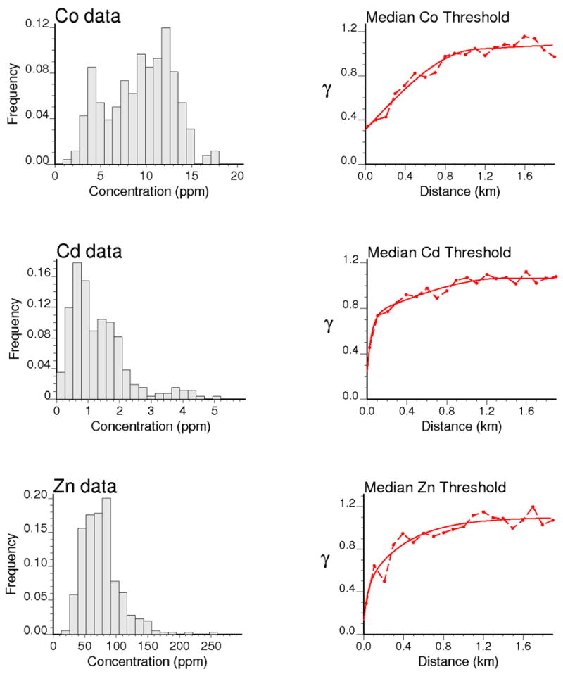
Histograms and median indicator semivariograms for the three heavy metals used in the sensitivity analysis.
As expected, increasing the number of thresholds attenuates the impact of the type of ccdf interpolation model on the prediction performances. For the two heavy metals with positively skewed distributions, the largest prediction errors are observed when performing a simple linear interpolation between fewer than 20 thresholds (Figures 13A–B). There is no substantial benefit in using more thresholds for cobalt that displays smaller relative prediction errors (16%) than cadmium (40%) or zinc (20%). Full and median indicator kriging yield very similar results, which suggests that the benefit of using threshold-specific semivariogram models is canceled out by the impact of more and greater order relation deviations, in particular as the number of thresholds increases (Figure 14). Regardless the type of indicator kriging, the largest proportion of order relation deviations is observed for cobalt, the metal with the strongest spatial structure (i.e. longest semivariogram range), leading to a higher likelihood of negative kriging weights caused by screening effect (Goovaerts, 1997). For example, median indicator kriging with the semivariogram models of Figure 12 (right column) generates 35% of negative kriging weights for cobalt, whereas this percentage is 0.02% for cadmium and 7.9% for zinc.
Figure 13.

Impact of the number of thresholds on the prediction accuracy and the goodness of the model of uncertainty obtained using indicator kriging and two types of ccdf interpolation models: crude linear interpolation between thresholds (left) and linear interpolation between tabulated bounds provided by the sample histogram (right). Solid lines correspond to results obtained for median indicator kriging where the same semivariogram model is used across all thresholds. Graphs (A) and (B) were rescaled by the average concentration (values for Cd were halved for graph clarity) so that they are comparable across metals and interpolation models.
Figure 14.

Impact of the number of thresholds on the frequency (A) and magnitude (B) of order relation deviations for three different heavy metals. Solid lines correspond to results obtained for median indicator kriging where the same semivariogram model is used across all thresholds.
As for the prediction errors, best results for the MSSR statistic (i.e. values closer to 1) are recorded when the number of thresholds exceeds 20, especially for Zn and Co using the crude linear interpolation model (Figures 13C–D). According to this criterion, median indicator kriging outperforms full indicator kriging for cobalt.
Unlike previous criteria, the goodness statistic does not improve as more thresholds are used (Figures 13E–F), although the decline is small in absolute terms. The slight increase in the width of the probability intervals (Figures 13G–H) is driven mainly by wider intervals for low probabilities (i.e. p < 0.2); see examples in Figures 1B and 11B. Overall the best results (i.e. more accurate and precise uncertainty models) are recorded for cobalt, which is expected since this metal displays the strongest spatial correlation.
5. Conclusions
This study demonstrated that nowadays indicator kriging with multiple thresholds is accessible and computationally tractable thanks to the development of automatic procedures for semivariogram fitting and the growing processing speed. In particular, the user should no longer feel restricted in using a maximum of nine thresholds for indicator coding, as typically done in many analyses. Using more thresholds attenuates the loss of information caused by the coding of continuous attributes into a set of binary indicators, which is a common criticism of the technique. Indicator kriging seems a better alternative to data transforms, since: (1) the transform procedure might be hard to automate (except for normal score transform, there is no guaranty that the transformed distribution will meet the requirements of the analysis) and (2) one-to-one transforms, such as normal score transform, require an arbitrary untie of censored data. This code should foster the application of indicator kriging in earth sciences and facilitates its optimal implementation by accounting for class-specific anisotropic patterns of spatial correlation, while allowing a quick assessment of the accuracy and precision of the non-parametric model of local uncertainty. This software should, however, not be used as a black-box and the reader is advised to analyze the semivariogram plots and cross-validation statistics to diagnose any potential problem in the application of the method.
According to the sensitivity analysis, for the dataset analyzed in this paper there appears to be little benefit in considering more than nine thresholds if the interpolation/extrapolation of discrete ccdf values is conducted using linear interpolation between tabulated bounds provided by the sample histogram. The pattern of spatial variability (i.e. range of indicator semivariogram model) seems to matter more than the use of threshold-specific semivariograms or the tenfold increase in the number of thresholds. The generalization of these preliminary conclusions will require repeating the analysis for other datasets with potentially larger differences in the spatial connectivity of small and large values. The benefit of using locally adaptive thresholds should also be explored.
Supplementary Material
Acknowledgments
This research was funded by grant R44-CA132347-01 from the National Cancer Institute. The views stated in this publication are those of the author and do not necessarily represent the official views of the NCI.
References
- Atteia O, Dubois JP, Webster R. Geostatistical analysis of soil contamination in the Swiss Jura. Environmental Pollution. 1994;86:315–327. doi: 10.1016/0269-7491(94)90172-4. [DOI] [PubMed] [Google Scholar]
- Barabás N, Goovaerts P, Adriaens P. Geostatistical assessment and validation of uncertainty for three-dimensional dioxin data from sediments in an estuarine river. Environmental Science & Technology. 2001;35(16):3294–3301. doi: 10.1021/es010568n. [DOI] [PubMed] [Google Scholar]
- Cattle JA, McBratney AB, Minasny B. Kriging method evaluation for assessing the spatial distribution of urban soil lead contamination. Journal of Environmental Quality. 2002;31:1576–1588. doi: 10.2134/jeq2002.1576. [DOI] [PubMed] [Google Scholar]
- Chu J. Fast sequential indicator simulation: beyond reproduction of indicator variograms. Mathematical Geology. 1996;28(7):923–936. [Google Scholar]
- Deutsch CV. Direct assessment of local accuracy and precision. In: Baafi EY, Schofield NA, editors. Geostatistics Wollongong ‘96. Kluwer Academic Publishers; Dordrecht: 1997. pp. 115–125. [Google Scholar]
- Deutsch CV, Lewis R. Advances in the practical implementation of indicator geostatistics. Proceedings of the 23rd International APCOM Symposium; Tucson, AZ, Society of Mining Engineers. 1992. pp. 169–179. [Google Scholar]
- Deutsch CV, Journel AG. GSLIB: Geostatistical Software Library and User’s Guide. 2. Oxford University Press; New York, NY: 1998. p. 369. [Google Scholar]
- Englund E, Sparks A. Geo-EAS 1.2.1 User’s Guide. EPA Report # 60018-91/008. EPA-EMSL; Las Vegas, NV: 1988. [Google Scholar]
- Goovaerts P. Comparative performance of indicator algorithms for modeling conditional probability distribution functions. Mathematical Geology. 1994;26(3):389–411. [Google Scholar]
- Goovaerts P. Geostatistics for Natural Resources Evaluation. Oxford University Press; New York, NY: 1997. p. 483. [Google Scholar]
- Goovaerts P. Geostatistical modelling of uncertainty in soil science. Geoderma. 2001;103:3–26. [Google Scholar]
- Goovaerts P, AvRuskin G, Meliker J, Slotnick M, Jacquez GM, Nriagu J. Geostatistical modeling of the spatial variability of arsenic in groundwater of Southeast Michigan. Water Resources Research. 2005;41(7):W07013 10.1029. [Google Scholar]
- Goovaerts P, Trinh HT, Demond AH, Towey T, Chang S-C, Gwinn D, Hong B, Garabrant D, Adriaens P. Geostatistical modeling of the spatial distribution of soil dioxin in the vicinity of an incinerator. 2. Verification and calibration study. Environmental Science & Technology. 2008;42(10):3655–3661. doi: 10.1021/es7024966. [DOI] [PMC free article] [PubMed] [Google Scholar]
- Journel AG. Nonparametric estimation of spatial distributions. Mathematical Geology. 1983;15(3):445–468. [Google Scholar]
- Lark RM, Ferguson RB. Mapping risk of soil nutrient deficiency or excess by disjunctive and indicator kriging. Geoderma. 2004;118(1):39–53. [Google Scholar]
- Lloyd CD, Atkinson PM. Assessing uncertainty in estimates with ordinary and indicator kriging. Computers and Geosciences. 2001;27(8):929–937. [Google Scholar]
- Pardo-Igúzquiza E. VARFIT: a Fortran-77 program for fitting variogram models by weighted least squares. Computers and Geosciences. 1999;25(3):251–261. [Google Scholar]
- Pardo-Igúzquiza E, Dowd PA. Multiple indicator cokriging with application to optimal sampling for environmental monitoring. Computers and Geosciences. 2005;31(1):1–13. [Google Scholar]
- Remy N, Boucher A, Wu J. Applied Geostatistics with SGEMS: A User’s Guide. Cambridge University Press; 2008. in press. [Google Scholar]
- Saito H, Goovaerts P. Geostatistical interpolation of positively skewed and censored data in a dioxin contaminated site. Environmental Science & Technology. 2000;34(19):4228–4235. [Google Scholar]
- Wackernagel H. Multivariate Geostatistics, 2nd completely revised edition. Berlin: Springer; 1998. p. 256. 1998. [Google Scholar]
Associated Data
This section collects any data citations, data availability statements, or supplementary materials included in this article.