Coupling the Level-Set Method with Molecular Mechanics for Variational Implicit Solvation of Nonpolar Molecules

Abstract

We construct a variational explicit-solute implicit-solvent model for the solvation of molecules. Central in this model is an effective solvation free-energy functional that depends solely on the position of solute-solvent interface and solute atoms. The total free energy couples altogether the volume and interface energies of solutes, the solute-solvent van der Waals interactions, and the solute-solute mechanical interactions. A curvature dependent surface tension is incorporated through the so-called Tolman length which serves as the only fitting parameter in the model. Our approach extends the original variational implicit-solvent model of Dzubiella, Swanson, and McCammon [Phys. Rev. Lett. 2006, 96, 087802 and J. Chem. Phys. 2006, 124, 084905] to include the solute molecular mechanics. We also develop a novel computational method that combines the level-set technique with optimization algorithms to determine numerically the equilibrium conformation of nonpolar molecules. Numerical results demonstrate that our new model and methods can capture essential properties of nonpolar molecules and their interactions with the solvent. In particular, with a suitable choice of the Tolman length for the curvature correction to the surface tension, we obtain the solvation free energy for a benzene molecule in a good agreement with experimental results.

I. Introduction

The interaction of biomolecules with an aqueous environment contributes significantly to the solvation free energy, structures, and functions of biomolecular systems. Efficient descriptions of such interactions are often given by implicit-solvent (or continuum-solvent) models.^1,2 In such models, the solvent molecules and ions are treated implicitly and their effects are coarse-grained. The effect of solvent is described through the continuum solute-solvent interface and related macroscopic quantities. These models are complementary to the more accurate but computationally expensive explicit-solvent models, such as molecular dynamics simulations which often provide sampled statistical information rather than direct descriptions of thermodynamics.

Most of the existing implicit-solvent models are built upon the concept of solvent-accessible surface (SAS) or solvent-excluded surface (SES) which can be defined in different ways.^3–7 In these models, the solvation free energy consists of the surface energy which is taken to be proportional to the area of a SAS or SES, and the electrostatic free energy determined by the Poisson-Boltzmann (PB)^8–10 or Generalized Born (GB)^11–13 description. While a SAS or SES based implicit-solvent approach has been extensively used and successful in many cases, its accuracy and general applicability are still questionable. One of the main issues here is the decoupling and separate descriptions of surface tension, dispersion, and the polar part of the free energy. Moreover, an ad hoc definition of SAS or SES can often lead to inaccurate free-energy estimation. It is additionally well established by now that cavitation free energies do not scale with surface area for high curvatures,^14,15 a fact of critical importance in the implicit-solvent modeling of hydrophobic interactions at molecular scales.¹⁶

In a recently developed variational implicit-solvent approach, Dzubiella, Swanson, and McCammon^17,18 proposed a mean-field approximation of the free energy of an underlying solvation system with an implicit solvent and fixed solute atoms as a functional of all possible solute-solvent interfaces. This free-energy functional couples both the nonpolar and polar contributions of the system. It allows for curvature correction of the surface tension to approximate the length-scale dependence of molecular hydration. Minimization of the free-energy functional determines an equilibrium solute-solvent interface and the minimum free energy of the solvation system. This stable, solute-solvent interface is an output of the theory. It results automatically from balancing the different contributions of the free energy.

Cheng, Dzubiella, McCammon, and Li¹⁹ first developed a level-set method for numerically capturing arbitrarily shaped equilibrium solute-solvent interfaces that minimize the solvation free-energy functional in the variational implicit-solvent model. In such a method, a possible solute-solvent interface is represented by the zero level-set (i.e., the zero level surface) of a level-set function; and an initial surface is evolved to reduce the free energy, eventually into an equilibrium solute-solvent interface. This relaxation process is determined by solving a time-dependent equation for the level-set function. The solute-solvent interface in each time step is then located as the zero-level surface of the level-set function. Here the time is not that in the real molecular dynamics. Rather it only represents an optimization step. We note that our level-set method for the relaxation of solute-solvent interfaces is quite different from that used in²⁰ which is only for generating a SAS or SES surface.

In the present work, we extend the original variational implicit-solvent model to include the degrees of freedom of all the solute atoms. More specifically, we construct a hybrid, variational explicit-solute implicit-solvent model to couple the coarse-grained solvent with the molecular mechanics of solute atoms. Our new effective free-energy functional depends not only on a solute-solvent interface but also positions of all the solute atoms. The free energy includes both the volume and surface energies of the solutes, the solute-solvent van der Waals interaction, and the electrostatic interaction. The Tolman curvature correction to the constant surface tension is incorporated through the so-called Tolman length which serves as the only fitting parameter in the model. The free energy also includes the van der Waals interaction as well as different kinds of molecular mechanical interactions among all the solute atoms. These mechanical interactions include the usual bond stretching, bending, and torsion. More terms can be added without difficulty. This explicit-solute implicit-solvent model is a more accurate and robust description of the structure of an underlying solvation system. Notice that we do not need to use solvation radii which are the fitting parameters in a usual SAS or SES type implicit-solvation model.

We also develop a level-set optimization method for the corresponding computer simulations. Our numerical free-energy minimization is carried out by solving two sets of time-dependent equations: one for the level-set function that determines the evolution of the solute-solvent interface and the other for the displacement of solute atoms. Our new level-set techniques include the numerical regularization for solving the level-set equation when instabilities occur, and a fast algorithm for numerically evaluating integrals of radially symmetric functions in the free-energy calculation. To efficiently and accurately couple the molecular interactions with the evolution of the solute-solvent interface, we choose carefully mobilities and optimization steps in our computation. While the time here means the optimization step, our approach can be used for the further development of a theory and simulation methods for real dynamics of solvation systems in the framework of variational implicit-solvent.

We apply our method to the solvation of the following nonpolar molecular systems: an artificial molecule of two atoms, an artificial molecule of four atoms, the ethane molecule C₂H₆, and the benzene molecule C₆H₆. Our extensive numerical results demonstrate that our approach can predict efficiently and accurately the free energy and structure of nonpolar molecules. In particular, with a suitably chosen Tolman length which is the only fitting parameter in our model and computation, we obtain a very good approximation of the experimentally measured solvation free energy for the benzene molecule. We are currently applying our theory and methods to polymers and large biomolecules. We are also working to include the electrostatics of an underlying system.

The rest of the paper is organized as follows: In Section II, we describe our hybrid explicit-solute implicit-solvent model that couples the original variational implicit-solvent with the solute molecular mechanics; In Section III, we present details of our level-set optimization algorithm. We also give formulas for the effective forces that are used as search directions in our numerical optimization. Some details of these formulas are given in the appendix; In Section IV, we report our results of numerical computations applied to some nonpolar molecular systems; Finally, in Section V, we discuss our results and draw some conclusions.

II. A Variational Explicit-Solute Implicit-Solvent Model

Our underlying system of molecules in a solution is divided geometrically into three parts: the solute region Ω_s, the solvent (e.g., water) region Ω_w, and the corresponding solute-solvent interface Γ which is the boundary of the solute region Ω_s as well as that of solvent region Ω_w, cf. Figure 1. Here we assume that there is a sharp interface that separates the solvent and solutes; and we treat the solvent as a continuum. We assume that there are N solute atoms in the system that are located at x₁, …, x_N inside Ω_s. These solute atoms are treated explicitly.

Fig. 1.

The geometry of a solvation system with an implicit solvent. The free energy depends on the position of solute-solvent interface Γ and solute atomic positions x₁, …,x_N.

Our basic assumption is that an experimentally observed equilibrium solvation system consists of a solute-solvent interface Γ and solute atoms located at x₁, …, x_N that together minimize an effective solvation free-energy functional. Along the line of variational implicit-solvent modeling of solvation systems,^17,18 we propose such an effective free-energy functional of a solute-solvent interface Γ and a set of solute atoms X = (x₁, …, x_N) to be

$$\begin{array}{l}G[\mathrm{\Gamma },X]=G_{\mathit{geom}}[\mathrm{\Gamma }]+G_{\mathit{vdW}}^{\mathit{sw}}[\mathrm{\Gamma },X]+G_{\mathit{elec}}[\mathrm{\Gamma },X]\\ +G_{\mathit{vdW}}^{\mathit{ss}}[X]+G_{\mathit{mech}}[X].\end{array}$$ (II.1)

The first term G_geom[Γ] is the geometrical contribution of the solute-solvent interface Γ. It has the form

$$G_{\mathit{geom}}[\mathrm{\Gamma }]=P\text{vol}({\mathrm{\Omega }}_s)+{\mathit{\int }}_{\mathrm{\Gamma }}\gamma \mathit{dS}.$$ (II.2)

Here the term Pvol(Ω_s), proportional to the volume of solute region Ω_s, is the energy of creating a cavity of solute against the pressure difference P between the solvent liquid and vapor phase. This term can often be neglected for nanometer sized solutes, since the pressure difference P is usually very small. The integral term in (II.2) is the surface energy, where γ is the surface tension. It is known that for systems of nanometer scale, the surface tension γ is no longer a constant. Corrections with curvature effect must be added. For a special case of a spherical solute, Tolman²¹ proposed that

$$\gamma =\frac{{\gamma }_0}{1+2\tau H},$$

where γ₀ is the constant surface tension for a planar solvent liquid-vapor interface, τ > 0 is a constant with τ often called the Tolman length,²¹ and H is the mean curvature defined to be the average of the two principal curvatures. Since the magnitude of 2τH is usually less than the unity, we use as in^18,19 the approximation (cf. also^22–24)

$$\gamma ={\gamma }_0(1-2\tau H).$$ (II.3)

The second term $G_{\mathit{vdW}}^{\mathit{sw}}[\mathrm{\Gamma },X]$ in the total free energy (II.1) is the nonpolar, van der Waals type interaction energy between the solute particles x₁, …,x_N and solvent molecules that are coarse-grained. As in^17–19 we define it to be

$$G_{\mathit{vdW}}^{\mathit{sw}}[\mathrm{\Gamma },X]={\rho }_0\sum _{i=1}^N{\mathit{\int }}_{{\mathrm{\Omega }}_w}{U}_{\mathit{sw}}(|\mathbf{\text{x}}-{\mathbf{\text{x}}}_i|)\mathit{dV},$$ (II.4)

where ρ₀ is the constant solvent density and U_sw = U_sw(r) is a pair-wise interaction potential. As in,^18,19 here we choose U_sw = U_sw(r) to be a Lennard-Jones potential

$$U_{\mathit{sw}}(r)=4{\epsilon }_{\mathit{sw}}\left[{\left(\frac{{\sigma }_{\mathit{sw}}}{r}\right)}^{12}-{\left(\frac{{\sigma }_{\mathit{sw}}}{r}\right)}^6\right].$$ (II.5)

The parameters ε_sw of energy and σ_sw of length can vary with different solute atoms as in the conventional force fields. Since the solvent is treated implicitly, the solute-solvent interaction energy (II.4) is expressed as an integral over the solvent region Ω_w.

The third term G_elec[Γ, X] in the total free energy (II.1) is the electrostatic free energy. In the mean-field approximation, this is given by^18,25

$$\begin{array}{l}{G}_{\mathit{elec}}[\mathrm{\Gamma },X]={\mathit{\int }}_{\mathrm{\Omega }}\left[{\rho }_f(\mathbf{\text{x}})\psi (\mathbf{\text{x}})-\frac{{\epsilon }_{\mathrm{\Gamma }}(\mathbf{\text{x}})}{8\pi }|\nabla \psi (\mathbf{\text{x}}){|}^2\right]\mathit{dV}\\ -{\beta }^{-1}\sum _{j=1}^M{c}_j^{\infty }{\mathit{\int }}_{{\mathrm{\Omega }}_s}\left(e^{-\beta qj\psi (\mathbf{\text{x}})}-1\right)\mathit{dV}.\end{array}$$

Here ψ = ψ(x) is the electrostatic potential usually determined by the Poisson-Boltzmann equation, ε_Γ = ε_Γ(x) is the dielectric coefficient that takes one constant value in the solute region Ω_s and a different constant value in the solvent region Ω_w, ρ_f = ρ_f(x) is the fixed charge density usually consisting of all solute point charges, β⁻¹ is the thermal energy, $c_j^{\infty }$ is the equilibrium concentration of the jth ionic species (a total of M is assumed), and q_j = ez_j with e the elementary charge and z_j the valence of jth ionic species in the solvent. More rigorous formulation of the electrostatic free energy can be found in²⁵ in which singularities in the potential ψ due to the point charges at solute atoms are carefully treated.

In this work, we only consider nonpolar systems and therefore set G_elec[Γ, X] = 0. This is our first step in developing our theory and methods of explicit-solute implicit-solvent modeling of biomolecular systems.

The fourth term $G_{\mathit{vdW}}^{\mathit{ss}}[X]$ in the total free energy (II.1) is the van der Waals interaction energy among solute atoms at x₁, …, x_N. It has the form

$$G_{\mathit{vdW}}^{\mathit{ss}}[X]=\sum _{(i,j)\prime }{U}_{\mathit{ss}}(|{\mathbf{\text{x}}}_i-{\mathbf{\text{x}}}_j|),$$ (II.6)

where the sum is taken over pairs of non-bonded solute atoms (x_i, x_j) with i < j and

$$U_{\mathit{ss}}(r)=4{\epsilon }_{\mathit{ss}}\left[{\left(\frac{{\sigma }_{\mathit{ss}}}{r}\right)}^{12}-{\left(\frac{{\sigma }_{\mathit{ss}}}{r}\right)}^6\right]$$ (II.7)

is a Lennard-Jones potential. The parameters ε_ss and σ_ss can vary with solute atoms.

The last term G_mech[X] in (II.1) is the energy of the molecular mechanical interactions among all the solute atoms x₁, …, x_N. This includes the usual bonding, bending, and torsion energies. Specifically, we define

$$\begin{array}{l}{G}_{\mathit{mech}}[X]=\sum _{(i,j)}{W}_{\mathit{bond}}({\mathbf{\text{x}}}_i,{\mathbf{\text{x}}}_j)\\ +\sum _{(i,j,k)}{W}_{\mathit{bend}}({\mathbf{\text{x}}}_i,{\mathbf{\text{x}}}_j,{\mathbf{\text{x}}}_k)\\ +\sum _{(i,j,k,l)}{W}_{\mathit{torsion}}({\mathbf{\text{x}}}_i,{\mathbf{\text{x}}}_j,{\mathbf{\text{x}}}_k,{\mathbf{\text{x}}}_l).\end{array}$$ (II.8)

Here the term Σ_(i,j) W_bond(x_i, x_j) accounts for the bonding energy of solute particles. The sum Σ_(i,j) is taken over all non redundant pairs of bonded solute atoms (x_i, x_j). The term Σ_(i,j,k,l) W_bend(x_i, x_j, x_k) in (II.8) accounts for the bending energy of solute atoms. The sum Σ_(i,j,k) is taken over all the non redundant triplets (x_i, x_j, x_k) such that both pairs of solute atoms (x_i, x_j) and (x_j, x_k) are bonded. The term Σ_(i,j,k,l) W_torsion(x_i, x_j, x_k, x_l) in (II.8) accounts for the torsion energy. The sum Σ_(i,j,k,l) is taken over all non redundant quadruples (x_i, x_j, x_k, x_l) such that (x_i, x_j), (x_j, x_k), (x_k, x_l) are all bonded. The forms of W_bond(x_i, x_j), W_bend(x_i, x_j, x_k), and W_torsion(x_i, x_j, x_k, x_l) are given in Appendix.

In summary, our proposed free-energy functional of a nonpolar (with G_elec[Γ, X] = 0) solvation system is given by (cf. (II.1), (II.2), (II.4), (II.6), and (A.1)–(A.3))

$$\begin{array}{l}G[\mathrm{\Gamma },X]=P\text{vol}({\mathrm{\Omega }}_s)+{\mathit{\int }}_{\mathrm{\Gamma }}\gamma \mathit{dS}\\ +{\rho }_0\sum _{i=1}^N{\mathit{\int }}_{{\mathrm{\Omega }}_w}{U}_{\mathit{sw}}(|\mathbf{\text{x}}-{\mathbf{\text{x}}}_i|)\mathit{dV}\\ +\sum _{(i,j)\prime }{U}_{\mathit{ss}}(|{\mathbf{\text{x}}}_i-{\mathbf{\text{x}}}_j|)\\ +\sum _{(i,j)}\frac{1}{2}{A}_{\mathit{ij}}{(r_{\mathit{ij}}-r_{0\mathit{ij}})}^2\\ +\sum _{(i,j,k)}\frac{1}{2}{B}_{\mathit{ijk}}({\theta }_{\mathit{ijk}}-{\theta }_{0\mathit{ijk}}{)}^2\\ +\sum _{(i,j,k,l)}[\frac{1}{4}(V_{\mathit{ijkl}}^{(1)}+2V_{\mathit{ijkl}}^{(2)}+V_{\mathit{ijkl}}^{(3)})\\ +\frac{1}{4}\left(V_{\mathit{ijkl}}^{(1)}-3V_{\mathit{ijkl}}^{(3)}\right){\mathrm{\Lambda }}_{\mathit{ijkl}}\\ -\frac{1}{2}{V}_{\mathit{ijkl}}^{(2)}{\mathrm{\Lambda }}_{\mathit{ijkl}}^2+V_{\mathit{ijkl}}^{(3)}{\mathrm{\Lambda }}_{\mathit{ijkl}}^3],\end{array}$$ (II.9)

supplemented by (II.3), (II.5), and (II.7).

III. A Level-Set Optimization Method

To find an equilibrium structure of an underlying solvation system that is a (local) minimizer of the free-energy functional (II.9), we select an initial solute-solvent interface and an initial set of solute atomic positions. We then start to move the interface and the set of solute atoms to relax the system.

To track the motion of the interface, we use the level-set method.^26–28 We represent the solute-solvent interface Γ = Γ(t) at time t as the zero level-set of a level-set function φ = φ(x, t), i.e., Γ(t) = {x : φ(x, t) = 0}. With this representation of the interface, we obtain the unit normal n = n(x, t), the mean curvature H = H(x, t), and the Gaussian curvature K = K(x, t) of a point x at the interface at time t

$$\begin{array}{ccc}\mathbf{\text{n}}=\frac{\nabla \phi }{|\nabla \phi |},& H=\frac{1}{2}\nabla \cdot \mathbf{\text{n}},& K=\mathbf{\text{n}}\end{array}\cdot \text{adj}(\text{He}(\phi ))\mathbf{\text{n}},$$ (III.1)

respectively, where He (φ) is the 3 × 3 Hessian matrix of the function φ whose entries are all the second order partial derivatives ${\partial }_{\mathit{ij}}^2\phi$ of the level-set function φ, and adj (He (φ)) is the adjoint matrix of the Hessian He(φ).

The level-set function is a solution to the level-set equation

$$\frac{\partial \phi }{\partial t}+v_n|\nabla \phi |=0,$$ (III.2)

where v_n = (dx(t)/dt) · n is the normal velocity of the moving interface Γ(t) at the point x = x(t). Notice that (d/dt)x(t) is the velocity of the point x(t) on the interface Γ(t). The equation (III.2) is derived from taking the time derivative of both sides of the equation φ(x, t) = 0 and using the chain rule.

To relax an underlying solvation system, we define the normal velocity v_n of the solute-solvent interface Γ(t) in such a way that the system moves in the steepest descent direction. Hence we define the normal velocity v_n to be the negative variation of the free energy G[Γ, X] with respect to the location change of the interface Γ:

$$v_n=-M_{\mathrm{\Gamma }}{\delta }_{\mathrm{\Gamma }}G[\mathrm{\Gamma },X],$$ (III.3)

where M_Γ > 0 is the mobility or relaxation factor which we take as a constant and δ_Γ denotes the first variation with respect to the location change of Γ. The variation δ_ΓG[Γ, X] defines a function on Γ, and is given by:^18,19

$$\begin{array}{l}{\delta }_{\mathrm{\Gamma }}G[\mathrm{\Gamma },X]=P+2{\gamma }_0[H(\mathbf{\text{x}})-\tau K(\mathbf{\text{x}})]\\ \begin{array}{cc}-{\rho }_0\sum _{i=1}^N{U}_{\mathit{sw}}(|\mathbf{\text{x}}-{\mathbf{\text{x}}}_i|)& \forall \mathbf{\text{x}}\in \mathrm{\Gamma },\end{array}\end{array}$$ (III.4)

where H(x) and K(x) are the mean curvature and Gaussian curvature of a point x ∈ Γ, respectively. (The Gaussian curvature is the product of the two principal curvatures.)

The motion of solute atoms is defined similarly to decrease the free energy. Therefore, the velocity of each of such atoms is given by

$$\begin{array}{cc}\frac{d{\mathbf{\text{x}}}_m(t)}{\mathit{dt}}=-M_m{\nabla }_{{\mathbf{\text{x}}}_m}G[\mathrm{\Gamma },X],& m=1,\cdots ,N,\end{array}$$ (III.5)

where M_m > 0 is a mobility or relaxation factor. Fix a particle x_m. The gradient of G[Γ, X] with respect to x_m is given by

$$\begin{array}{l}{\nabla }_{{\text{X}}_m}G[\mathrm{\Gamma },\mathbf{\text{x}}]={\rho }_0{\mathit{\int }}_{{\mathrm{\Omega }}_w}{U}_{\mathit{sw}}^{\prime }(|{\mathbf{\text{x}}}_m-\mathbf{\text{x}}|)\frac{{\mathbf{\text{x}}}_m-\mathbf{\text{x}}}{|{\mathbf{\text{x}}}_m-\mathbf{\text{x}}|}\mathit{dV}\\ +\sum _{(i,j)\prime }{\delta }_{\mathit{mi}}{U}_{\mathit{ss}}^{\prime }(|{\mathbf{\text{x}}}_i-{\mathbf{\text{x}}}_j|)\frac{{\mathbf{\text{x}}}_i-{\mathbf{\text{x}}}_j}{|{\mathbf{\text{x}}}_i-{\mathbf{\text{x}}}_j|}\\ +\sum _{(i,j)}{\delta }_{\mathit{mi}}{A}_{\mathit{ij}}(r_{\mathit{ij}}-r_{0ij})\frac{{\mathbf{\text{x}}}_i-{\mathbf{\text{x}}}_j}{|{\mathbf{\text{x}}}_i-{\mathbf{\text{x}}}_j|}\\ +\sum _{(i,j,k)}{\nabla }_{{\mathbf{\text{x}}}_m}{W}_{\mathit{bend}}({\mathbf{\text{x}}}_i,{\mathbf{\text{x}}}_j,{\mathbf{\text{x}}}_k)\\ +\sum _{(i,j,k,l)}{\nabla }_{{\mathbf{\text{x}}}_m}{W}_{\mathit{torsion}}({\mathbf{\text{x}}}_i,{\mathbf{\text{x}}}_j,{\mathbf{\text{x}}}_k,{\mathbf{\text{x}}}_l),\end{array}$$ (III.6)

where δ_mi is 1 if i = m and 0 if i ≠ m. The derivatives ∇_xm W_bend(x_i, x_j, x_k) and ∇_xm W_torsion(x_i, x_j, x_k, x_l) are given in the appendix.

In each time step of relaxation, we solve the system of equations (III.2) and (III.5) and find the solute-solvent interface by locating all the points at which the level-set function φ vanishes. In solving these equations, we use the first variation δ_ΓG[Γ, X] and the gradients ∇_x G[Γ, X] that are given by (III.4), (III.6), (A.4), and (A.8), together with (A.5)–(A.7) and (A.9)–(A.15).

Notice that by a series of formal calculations we have that

$$\begin{array}{l}\frac{d}{\mathit{dt}}G[\mathrm{\Gamma },X]\\ ={\delta }_{\mathrm{\Gamma }}G[\mathrm{\Gamma },X]v_n+\sum _{m=1}^N{\nabla }_{{\mathbf{\text{x}}}_m}G[\mathrm{\Gamma },X]\frac{d{\mathbf{\text{x}}}_m(t)}{\mathit{dt}}\\ =-M_{\mathrm{\Gamma }}[{\delta }_{\mathrm{\Gamma }}G[\mathrm{\Gamma },X]{]}^2-\sum _{m=1}^N{M}_m|{\nabla }_{{\mathbf{\text{x}}}_m}G[\mathrm{\Gamma },X]{|}^2\\ \le 0.\end{array}$$

This confirms that the free energy decays.

We have developed a numerical algorithm that combines the level-set method and optimization techniques to numerically find solutions of the system (III.2) and (III.5). Our numerical algorithm consists of the following steps:

1. Choose a computational box, a cube in ℝ³, and discretize the box with a uniform finite-difference grid. Initialize the level-set function φ and position of solute atoms x₁, …, x_N. We place the initial solute-solvent interface a few grid points away from the boundary of the computational box, just so that we can solve the level-set equation more accurately, cf. Step (2). One choice of the initial level-set function is

   $$\phi (\mathbf{\text{x}})=\underset{1\le i\le N}{min}(|\mathbf{\text{x}}-{\mathbf{\text{x}}}_i|-r_i),$$ (III.7)

   where r_i > 0 (i = 1, …, N) are preselected numbers. Notice that the solute atoms are not necessarily placed at grid points.

2. Calculate and extend the normal velocity v_n using the formula (III.3) and (III.4). The extension of the normal velocity v_n from the interface Γ(t) to the computational box is necessary for solving the level-set equation (III.2) on the computational box. In our current implementation, we use the level-set function φ and the formulas in (III.1) to define the mean curvature H and Gaussian curvature K all over the computational domain. Therefore we only extend the Lennard-Jones potential part in the normal velocity, the last term in (III.3). We extend this part to a narrow band of the interface by constant in the normal direction of the interface.

3. Solve the level-set equation (III.2). We use the forward Euler method to discretize the time derivative in the level-set equation. The normal velocity v_n consists of two parts. One is from the motion of the surface energy and is more of a parabolic type term in the equation. The other is from the solute-water interaction and only gives rise to a lower order term. We thus use the central differencing scheme to discretize the first part and an upwinding scheme for the second part. We choose our time step Δt to be of the order of (Δx)² to satisfy the CFL stability condition. A simple linearization analysis shows that the level-set equation becomes backward parabolic if 1 − 2τκ₁ < 0 or 1 − 2τκ₂ < 0, where κ₁ and κ₂ are the two principle curvatures. If this occurs, then we numerically change the parameter τ to regularize the interface motion.

4. Reinitialize the level-set function. This step is necessary to keep the level-set function away from being too flat or steep. If the level-set function is φ₀ in the current step, we solve the equation

   $$\frac{\partial \phi }{\partial t}=\text{sign}({\phi }_0)(1-|\nabla \phi |)$$

   to obtain a new approximation of the level-set function, where sign(φ₀) is the sign of φ₀;

5. Calculate the velocity of solute atoms using the formula (III.6). We evaluate the integral term in (III.6) as follows: For each solute atom x_m, we choose a ball B(x_m, r_m) centered at the x_m with a radius r_m. This ball is small enough so that it is completely contained in the solute region Ω_s. Then we compute the integral term in (III.6) using the formula

   $$\begin{array}{l}{\mathit{\int }}_{{\mathrm{\Omega }}_w}{U}_{\mathit{sw}}^{\prime }(|{\mathbf{\text{x}}}_m-\mathbf{\text{x}}|)\frac{{\mathbf{\text{x}}}_m-\mathbf{\text{x}}}{|{\mathbf{\text{x}}}_m-\mathbf{\text{x}}|}\mathit{dV}\\ ={\mathit{\int }}_{{ℝ}^3\backslash B({\mathbf{\text{x}}}_m,r_m)}{U}_{\mathit{sw}}^{\prime }(|{\mathbf{\text{x}}}_m-\mathbf{\text{x}}|)\frac{{\mathbf{\text{x}}}_m-\mathbf{\text{x}}}{|{\mathbf{\text{x}}}_m-\mathbf{\text{x}}|}\mathit{dV}\\ ={\mathit{\int }}_{{\mathrm{\Omega }}_s\backslash B({\mathbf{\text{x}}}_m,r_m)}{U}_{\mathit{sw}}^{\prime }(|{\mathbf{\text{x}}}_m-\mathbf{\text{x}}|)\frac{{\mathbf{\text{x}}}_m-\mathbf{\text{x}}}{|{\mathbf{\text{x}}}_m-\mathbf{\text{x}}|}\mathit{dV},\end{array}$$

   where the integral over ℝ³ \ B(x_m, r_m) (the region complement to the ball B(x_m, r_m)) is calculated analytically;

6. Update the position of each solute atom x_i by the formula (III.5). We use the forward Euler method for updating the atom positions. Our time step in solving the equations (III.5) for the motion of solute atoms is much smaller than that in solving the level-set equation (III.2);

7. Calculate the total free energy (II.9). To calculate the solute-solvent interaction term (II.4) in the total free energy (II.9), we use the method same as described in Step (5). In testing our method of calculating the total energy for a one-atom system, we found that our method is second-order accurate;

8. Go to Step (2).

IV. Numerical Tests and Applications

A. A two-atom molecule

We consider an artificial molecular system of two atoms. The thermodynamic and LJ parameters we use are mostly taken from¹⁹ which are for the system of two xenon atoms. These parameters are: the pressure difference P = 0 bar (an approximation), the constant surface tension γ₀ = 0.174 k_BT/Ų, the Tolman length τ = 1.3 Å, the water density ρ₀ = 0.033 Å⁻³, the solute-water Lennard-Jones parameters σ = 3.57 Å and ε = 0.431 k_BT, the solute-solute Lennard-Jones parameters σ = 3.57 Å and ε = 0.147 k_BT, the temperature T = 298 K. We additionally introduce an intra-bond with the spring constant in the bond stretching energy A = 800 k_BT/Ų, and the equilibrium bond length r₀ = 3 Å. To test our method, we include both the bonding and Lennard-Jones interaction between the two atoms.

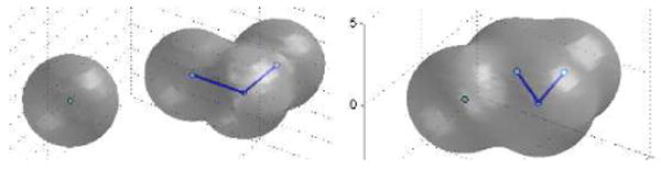
We test two possible cases. In the first case, we place initially the two solute atoms far away from each other so that their distance is much larger than the equilibrium bond length. We also set the initial solute-solvent interface to be two separated spheres that are centered at the two solute atoms, respectively. A few snapshots of the system during the relaxation are gathered in Figure 2. We see that those two initially separated spheres merge and the distance between the two solute atoms gets closer, and then the system reaches an equilibrium state. Notice from the lower left snapshot in Figure 2 that the solute-solvent interface is not in equilibrium with respect to the two atoms. This means that the system is relaxed through the coupling of both the interface motion and atomic motion. In Figure 3 we plot the total free energy vs. the computational step. It is clear that the free energy decays in each step.

Fig. 2.

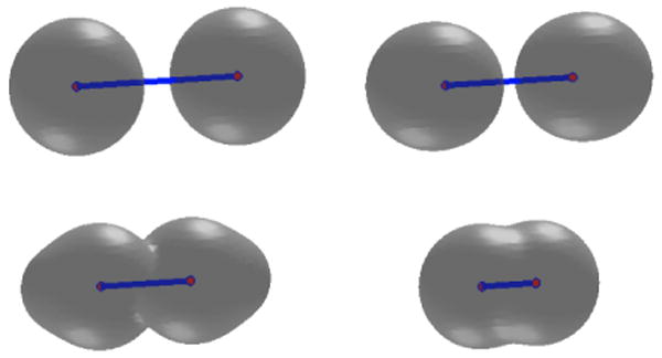
The level-set optimization of a two-atom system. The initial solute-solvent interface consists of two separated spheres. Order of snapshots: from left to right and from top to bottom.

Fig. 3.

The free energy (kcal/mol) vs. the computational step in a level-set optimization for the two-atom system with the initial solute-solvent interface consisting of two separated spheres, cf. Figure 2.

In the second case, we place initially the two solute atoms very close to each other so that their distance is smaller than the equilibrium distance. We also set the initial solute-solvent interface to be a large surface that encloses both of the atoms. A few snapshots from our numerical relaxation are shown in Figure 4. The decay of the free energy in our numerical computation is shown in Figure 5. We notice that the free energy decays very fast in this case. This is due to very strong repulsion modeled by the Lennard-Jones potential.

Fig. 4.

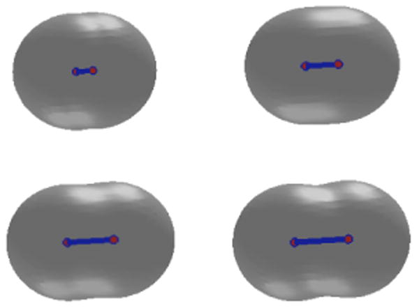
The level-set optimization of a two-atom system. The two atoms are initially close and then move apart from each other. Order of snapshots: from left to right and from top to bottom.

Fig. 5.

The free energy (kcal/mol) vs. the computational step in a level-set optimization for the two-atom system with the initial solute-solvent interface consisting of a single surface containing the two atoms, cf. Figure 4.

Through this test example, we see that our level-set method works well in capturing topological changes of surfaces during relaxation. We also find that the final free energy values for the two different cases are nearly the same: 6.36397 k_BT and 6.36652 k_BT, respectively, with an error of 0.00255 k_BT.

Our results show a strong contribution of the molecular mechanical force in the relaxation of the system. To understand the solvent influence, and particularly, how the motion of solute-solvent interface affects that of solute particles, we turn off the particle-particle interaction in the two-atom system. We perform two tests. In the first test summarized in Figure 6, we set the initial center-to-center distance between the two atoms to be 5 Å. This is in the range between 0 to about 6 Å of attraction of the two atoms as shown in Figure 1 of our previous work.¹⁹ Such attraction results from the minimization of the interfacial energy. Since there is no atom-atom interaction, the solute-solvent interaction pushes these two atoms together. The sequence of snapshots in Figure 6 demonstrate clearly that the solvent contributes significantly to the motion of solute particles.

Fig. 6.

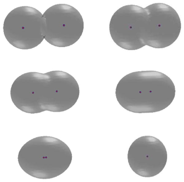
Snapshots of a relaxing system of two non-interacting particles. Order: left to right and top to bottom.

In the second test, we set the initial center-to-center distance between the two atoms to be 6.8 Å. This is in a range of (weak) repulsion as predicted in our previous work.¹⁹ The non-interacting two atoms are then pushed away by the solute-solvent interaction, cf. Figure 7. Notice that the surface area for the initial, connected two-sphere system (Figure 7, left) increases to that of final, separated two-sphere system (Figure 7, right). Such increasing of surface area compensates the solute-solvent interaction. It obviously can not be captured by a SAS/SES type model, in which the nonpolar part of the free energy is the surface energy, proportional to the surface area.

Fig. 7.

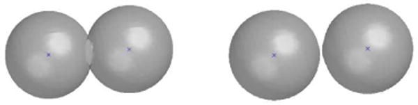
Two non-interacting particles relax with increasing surface area.

B. A four-atom molecule

We consider an artificial molecular system of four atoms x₁, …, x₄ to test how our method can handle the bending energy and the solute-solute van der Waals interaction in addition to the variational implicit-solvent. We put the pairs (x₁, x₂) and (x₂, x₃) in their equilibrium bonding position and arrange the angle between x₂x₁ and x₂x₃ slightly different from an equilibrium angle. We also put x₄ relatively far away from the first three atoms. The atom x₄ interacts with the other three atoms via a Lennard-Jones potential. Figure 8 (left) shows the initial conformation and Figure 8 (right) the relaxed conformation of this system. It is clear that the fourth atom moves closer to the three-atom group while the angle between x₂x₁ and x₂x₃ is relaxed to its equilibrium value.

Fig. 8.

Left: Initial positions of the solute-solvent interface and solute atoms. Right: The relaxed positions of the solute-solvent interface and solute atoms.

C. An ethane molecule

We consider an ethane molecule C₂H₆ in water and take from^29–31 the solute atomic positions and force field parameters. Other parameters are: the pressure differencing P = 0 bar, the constant surface tension γ₀ = 0.174 k_BT/Ų, the Tolman length τ = 1.3 Å, the water density ρ₀ = 0.033 Å⁻³, the carbon-water Lennard-Jones parameters σ = 3.4767 Å and ε = 0.2311 k_BT, the hydrogen-water Lennard-Jones parameters σ = 3.1017 Å and ε = 0.0989 k_BT.

We construct an initial conformation of the ethane molecule from its equilibrium in which three hydrogen-carbon bonds with respect to one of the carbon atom are rotated 20 degrees. During the level-set relaxation, these three hydrogen atoms rotate back to their equilibrium positions. The solute-solvent interface also moves to its equilibrium position. Figure 9 displays a few snapshots of our numerical results. Figure 10 is a plot of the free energy in each step of our numerical computation.

Fig. 9.

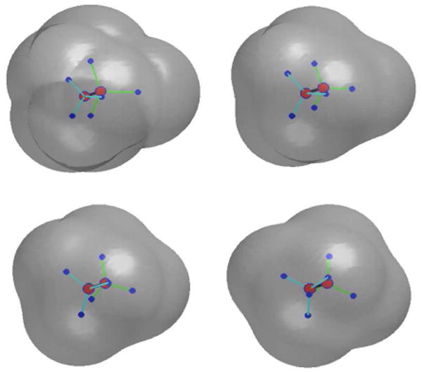
The level-set relaxation of the ethane molecule. Order of snapshots: from first row to second and from left to right in each row.

Fig. 10.

A plot of the total free energy (kcal/mol) vs. computational step in the level-set optimization for the ethane molecule.

D. A benzene molecule

We consider a benzene molecule C₂H₆ in water and take from^29–31 the solute atomic positions and force field parameters. Other parameters are the same as those for an ethane molecule.

We construct an initial conformation of the benzene molecule from its equilibrium in which all the atoms are on the same plane. We then fix a pair of C-atoms that are opposite in the hexagonal ring. We pull up one of these two C-atoms and pull down the other C-atom to form the initial positions of all the atoms. We also use (III.7) to define an initial solute-solvent interface. During the process of our level-set relaxation, those two carbon atoms move back to their equilibrium positions. The solute-solvent interface also moves to its equilibrium position. Figure 11 displays a few snapshots of our numerical results. Figure 12 is a plot of the free energy in each step of our numerical computation.

Fig. 11.

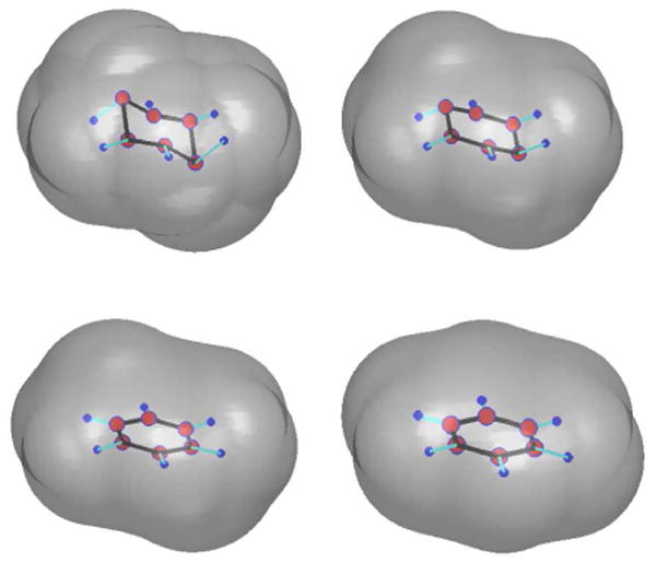
The level-set relaxation of the benzene molecule. Order of snapshots: from first row to second and from left to right in each row.

Fig. 12.

A plot of the total free energy (kcal/mol) vs. computational step in the level-set optimization for the benzene molecule.

We have tried various values of the Tolman length τ. For τ = 1 Å, we find that the free energy (surface energy and the benzene-water interaction energy) is 1.98 kcal/mol. Using a Poisson-Boltzmann solver, we find the polar part of the solvation energy is −2.92 kcal/mol. Therefore, our estimate of the solvation energy is −0.94 kcal/mol. The experimental value of this solvation energy is −0.89 kcal/mol.

Our PB calculation was done by impact version 50112 (released by Schrodinger, LLC) with default settings (PB grid resolution was set to high) with OPLS2005 forcefield. Since we have not implemented our own PB solver, the optimized surface was not used to define the boundary. But the benzene molecule is small and geometrically simple, we do not expect the variational surface to be drastically different from a traditional SAS. Therefore, we believe the polar energy from traditional PB solver using a SAS is consistent with our variational implicit-solvent description of the benzene molecule.

V. Conclusions

In this work, we construct a hybrid explicit-solute implicit-solvent model for molecular solvation. The key quantity in this model is an effective free-energy functional of positions of solute atoms and solute-solvent interface. The free energy couples both the polar and non-polar contributions and also includes the molecular mechanical interactions. Minimization of this free-energy functional determines an equilibrium molecular structure and the solvation free energy. We also develop a level-set optimization method to numerically minimize the free-energy functional and to obtain equilibrium solute-solvent interface and positions of solute atoms. In our method, both a trial solute-solvent interface and a set of trial solute atoms move in the steepest descent direction of reducing the total free energy of the system. Our numerical results for the solvation of some molecules demonstrate that our model and methods can capture topological changes of the solute-solvent interface as well as the coupling between such an interface motion and molecular mechanical interactions.

We emphasize again that we model a relaxation process or free-energy minimization rather than the real dynamics of an underlying molecular system.

For each of the small, non-polar systems that we have tested and reported here, our level-set relaxation only took a few minutes. The actual exact computational time is affected by several factors such as the number of grid points (the resolution) and the choice of initial surface. It is clear, however, that our approach is in general computationally more costly than a SAS/SES type implicit-solvent model, since we need to evolve a surface to its equilibrium state. Nevertheless, we have been developing several new level-set techniques that can speed up our computations. One of such techniques is the local level-set method. It can reduce the complexity of a three-dimensional problem to that of a two-dimensional one.

As noted before the only fitting parameter in our model is the Tolman length τ. We find that the free energy calculation is sensitive to the choice of the Tolman length. Our experience is that τ = 1 Å is a good value for many molecular systems. Figure 13 plots the nonpolar part of the minimum solvation energy (the surface energy plus the solute-solvent interaction energy) vs. the Tolman length τ for the benzene molecule. We can see a perfect linear dependence of the the nonpolar part of the solvation energy on the Tolman length. This indicates the existence of an optimal Tolman length. It also points to the fact that that the minimized interface hardly changes with the fitting parameter τ for this particular example, and that the free energy is directly proportional to τ as can be predicted from (II.2) and (II.3). In general, especially for larger molecules with a higher dispersion and complexity in curvature, the relation will be qualitatively different. In future, we hope a more sophisticated free-energy functional can be proposed in order to fix an optimal value of τ once and for all, independent of the particular solute system.

Fig. 13.

The sum of the surface energy and benzene-water interaction energy vs. the Tolman length τ.

In a SAS implicit-solvent model, the size effect of solvent molecules is described through the probing solvent molecule used in defining the SAS. In our variational implicit-solvent model (VISM), such size effect is reflected in the solute-solvent interaction, cf. (II.4). In general, an implicit or “continuum” solvent model is, per definition and how the name implies, not able to explicitly describe the finite size of solvent molecules. Implicitly, these effects are typically considered in fitting parameters. In a solvation system, the solvent-solute interface itself is not a sharp boundary but has a width of solvent molecule size (∼ 3 Å). Thus, the “right” interface location basically does not exist within a few Angstroms. Consequently, it is hard to compare precisely a SAS/SES type implicit-solvent model to our VISM. The final goal must be to evaluate the correct free energy from any of these surface definitions; “correct” in the sense that they are quantitative in comparison to bench-marking experiments or explicit-solvent molecular dynamics simulations. The virtue of the VISM is that the interface is defined in a physically reasonable way and allows the interface—for every configuration—to respond to local solute geometry and energetic potentials, and can hopefully provide accurate free energies with only very few fitting parameters (in contrast to established implicit models). If the capillary evaporation (“dewetting” or “drying”) between solutes takes places, then the VISM interface can be very different to the a priori defined SAS/SES interfaces as the latter do not capture solvent evaporation.

Our immediate next step is to add the electrostatic part of the free energy into our model and develop a corresponding level-set method. The electrostatic free energy is often described by the Poisson-Boltzmann (PB) or Generalized Born (GB) method in which the solute-solvent interface is used as the dielectric boundary. Our first step will be the development of a GB-like approach to efficiently calculate the effective electrostatic surface force (only its normal component) at each point of the evolving solure-solvent interface. This force will be used as the normal velocity in the level-set relation of the solute-solvent interface. Next we will develop a fast PB solver and couple it with our level-set code. Solving the nonlinear PB equation in each step of level-set relaxation can be very slow. To speed up our computations, we can in each step linearize the PB equation around the previous PB solution. Thus, in each step, we need only to solve a linearized PB equation. (This linearized equation is different from the Debye-Hückel equation.) Moreover, we do not need to solve very accurately the PB equation very step, since dewetting regions can be mainly captured by the surface energy term.

Besides adding the electrostatics into our models and methods, we will also apply our model and methods to larger systems of polymers and biomolecules. Further, we will apply our theory and methods to the calculation of surface forces of solute-solvent interfaces that can be used in Brownian dynamics simulations of biomolecules.

Appendix A

Molecular mechanical interactions and force calculations

We summarize in this appendix the molecular mechanical interaction energies and their derivatives.

For a given pair of bonded solute atoms (x_i, x_j), the bonding energy is given by the harmonic approximation

$$W_{\mathit{bond}}({\mathbf{\text{x}}}_i,{\mathbf{\text{x}}}_j)=\frac{1}{2}{A}_{\mathit{ij}}{(r_{\mathit{ij}}-r_{0\mathit{ij}})}^2,$$ (A.1)

where A_ij is a spring constant characterizing the equilibrium bonding strength, r_ij = |x_i − x_j| is the distance between x_i and x_ij, and r_0ij is the corresponding equilibrium distance.

For a triplet (x_i, x_j, x_k) with (x_i, x_j) and (x_j, x_k) both bounded, the bending energy is given by the harmonic approximation

$$W_{\mathit{bend}}({\mathbf{\text{x}}}_i,{\mathbf{\text{x}}}_j,{\mathbf{\text{x}}}_k)=\frac{1}{2}{B}_{\mathit{ijk}}{({\theta }_{\mathit{ijk}}-{\theta }_{0\mathit{ijk}})}^2,$$ (A.2)

where B_ijk is a constant parameter depending in general on (i, j, k), θ_ijk is the angle between the vectors r_ji = x_i − x_j and r_jk = x_k − x_j, and θ_0ijk is the corresponding equilibrium angle constrained by 0 ≤ θ_0ijk ≤ π for all (i, j, k).

For a quadruple (x_i, x_j, x_k, x_l) such that (x_i, x_j), (x_j, x_k), (x_k, x_l) are all bonded, the torsion angle φ_ijkl is the angle between the plane determined by x_i, x_j, x_k and that determined by x_j, x_k, x_l. The torsion energy is (see, e.g.,32)

$$\begin{array}{l}{W}_{\mathit{torsion}}({\mathbf{\text{x}}}_i,{\mathbf{\text{x}}}_j,{\mathbf{\text{x}}}_k,{\mathbf{\text{x}}}_l)=\frac{1}{2}{V}_{\mathit{ijkl}}^{(1)}[1-cos(\pi {\phi }_{\mathit{ijkl}})]\\ +\frac{1}{2}{V}_{\mathit{ijkl}}^{(2)}[1+cos(2\pi {\phi }_{\mathit{ijkl}})]\\ +\frac{1}{2}{V}_{\mathit{ijkl}}^{(3)}[1-cos(3\pi {\phi }_{\mathit{ijkl}})]\end{array}$$ (A.3)

where $V_{\mathit{ijkl}}^{(1)},V_{\mathit{ijkl}}^{(2)}$, and $V_{\mathit{ijkl}}^{(3)}$ are constants.

Fix x_i, x_j, and x_k. Denote by r_ji = x_i − x_j the vector from x_j to x_i for any i and j and by r_ji = |r_ji| the length of this vector. Routine calculations lead to

$$\nabla W_{\mathit{bend}}({\mathbf{\text{x}}}_i,{\mathbf{\text{x}}}_j,{\mathbf{\text{x}}}_k)=B_{\mathit{ijk}}({\theta }_{\mathit{ijk}}-{\theta }_{0\mathit{ijk}})\nabla {\theta }_{0\mathit{ijk}},$$ (A.4)

where

$${\nabla }_{x_i}{\theta }_{\mathit{ijk}}=\frac{1}{sin{\theta }_{\mathit{ijk}}}\left(\frac{{\mathbf{\text{r}}}_{\mathit{\text{ji}}}\cdot {\mathbf{\text{r}}}_{\mathit{\text{jk}}}}{r_{\mathit{\text{ji}}}^3{r}_{\mathit{\text{jk}}}}{\mathbf{\text{r}}}_{\mathit{\text{ji}}}-\frac{1}{r_{\mathit{\text{ji}}}{r}_{\mathit{\text{jk}}}}{\mathbf{\text{r}}}_{\mathit{\text{jk}}}\right),$$ (A.5)

$${\nabla }_{{\mathbf{\text{x}}}_k}{\theta }_{\mathit{ijk}}=\frac{1}{sin{\theta }_{\mathit{ijk}}}\left(\frac{{\mathbf{\text{r}}}_{\mathit{\text{ji}}}\cdot {\mathbf{\text{r}}}_{\mathit{\text{jk}}}}{r_{\mathit{\text{jk}}}^3{r}_{\mathit{\text{ji}}}}{\mathbf{\text{r}}}_{\mathit{\text{jk}}}-\frac{1}{r_{\mathit{\text{ji}}}{r}_{\mathit{\text{jk}}}}{\mathbf{\text{r}}}_{\mathit{\text{ji}}}\right),$$ (A.6)

$$\begin{array}{l}{\nabla }_{{\mathbf{\text{x}}}_j}{\theta }_{\mathit{ijk}}=\frac{1}{sin{\theta }_{\mathit{ijk}}}[\left(\frac{1}{r_{\mathit{\text{ji}}}{r}_{\mathit{\text{jk}}}}-\frac{cos{\theta }_{\mathit{ijk}}}{r_{\mathit{\text{ji}}}^2}\right){\mathbf{\text{r}}}_{\mathit{\text{ji}}}\\ +\left(\frac{1}{r_{\mathit{\text{ji}}}{r}_{\mathit{\text{jk}}}}-\frac{cos{\theta }_{\mathit{ijk}}}{r_{\mathit{\text{jk}}}^2}\right){\mathbf{\text{r}}}_{\mathit{\text{jk}}}].\end{array}$$ (A.7)

For a given quadruple (x_i, x_j, x_k, x_l), we denote

$$\begin{array}{l}{\mathbf{\text{r}}}_1={\mathbf{\text{r}}}_{\mathit{\text{ij}}},{\mathbf{\text{r}}}_2={\mathbf{\text{r}}}_{\mathit{\text{jk}}},{\mathbf{\text{r}}}_3={\mathbf{\text{r}}}_{\mathit{\text{kl}},}\\ \mathbf{\text{u}}={\mathbf{\text{r}}}_1\times {\mathbf{\text{r}}}_2,\mathbf{\text{v}}={\mathbf{\text{r}}}_2\times {\mathbf{\text{r}}}_{3,}\\ \phi ={\phi }_{\mathit{ijkl}},\mathrm{\Lambda }={\mathrm{\Lambda }}_{\mathit{ijkl}}=cos\phi =\frac{\mathbf{\text{u}}\cdot \mathbf{\text{v}}}{\left|\mathbf{\text{u}}\right|\left|\mathbf{\text{v}}\right|},\\ V^{(n)}=V_{\mathit{ijkl}}^{(n)},n=1,2,3.\end{array}$$

It follows from (A.3) and a series of elementary calculations that

$$\begin{array}{l}{\nabla }_{{\mathbf{\text{r}}}_m}{W}_{\mathit{torsion}}({\mathbf{\text{x}}}_i,{\mathbf{\text{x}}}_j,{\mathbf{\text{x}}}_k,{\mathbf{\text{x}}}_l)\\ =[-\frac{1}{2}\left(V^{(1)}-3V^{(3)}\right)-2V^{(2)}\mathrm{\Lambda }\\ +6V^{(3)}{\mathrm{\Lambda }}^2]{\nabla }_{{\mathbf{\text{x}}}_m}\mathrm{\Lambda },\end{array}$$ (A.8)

where ∇_xm Λ = 0 if m is not one of i, j, k, or l, and

$${\nabla }_{{\mathbf{\text{x}}}_i}\mathrm{\Lambda }=-{\nabla }_{{\mathbf{\text{r}}}_1}\mathrm{\Lambda },$$ (A.9)

$${\nabla }_{{\mathbf{\text{x}}}_j}\mathrm{\Lambda }={\nabla }_{{\mathbf{\text{r}}}_1}\mathrm{\Lambda }-{\nabla }_{{\mathbf{\text{r}}}_2}\mathrm{\Lambda },$$ (A.10)

$${\nabla }_{{\mathbf{\text{x}}}_k}\mathrm{\Lambda }={\nabla }_{{\mathbf{\text{r}}}_2}\mathrm{\Lambda }-{\nabla }_{{\mathbf{\text{r}}}_3}\mathrm{\Lambda },$$ (A.11)

$${\nabla }_{{\mathbf{\text{x}}}_l}\mathrm{\Lambda }={\nabla }_{{\mathbf{\text{r}}}_3}\mathrm{\Lambda },$$ (A.12)

and

$${\nabla }_{{\mathbf{\text{r}}}_1}\mathrm{\Lambda }=\frac{({\mathbf{\text{r}}}_1\cdot \mathbf{\text{v}}){\left|{\mathbf{\text{r}}}_2\right|}^2}{{\left|\mathbf{\text{u}}\right|}^3\left|\mathbf{\text{v}}\right|}\mathbf{\text{u}},$$ (A.13)

$${\nabla }_{{\mathbf{\text{r}}}_2}\mathrm{\Lambda }=\frac{{\mathbf{\text{r}}}_1\cdot \mathbf{\text{v}}}{{\left|\mathbf{\text{u}}\right|}^3{\left|\mathbf{\text{v}}\right|}^3}[({\mathbf{\text{r}}}_1\cdot {\mathbf{\text{r}}}_2){\left|\mathbf{\text{v}}\right|}^2\mathbf{\text{u}}+({\mathbf{\text{r}}}_2\cdot {\mathbf{\text{r}}}_3){\left|\mathbf{\text{u}}\right|}^2\mathbf{\text{v}}],$$ (A.14)

$${\nabla }_{{\mathbf{\text{r}}}_3}\mathrm{\Lambda }=-\frac{({\mathbf{\text{r}}}_1\cdot \mathbf{\text{v}}){\left|{\mathbf{\text{r}}}_2\right|}^2}{\left|\mathbf{\text{u}}\right|{\left|\mathbf{\text{v}}\right|}^3}\mathbf{\text{v}}.$$ (A.15)

References

- 1.Roux B, Simonson T. Biophys Chem. 1999;78:1–20. doi: 10.1016/s0301-4622(98)00226-9. [DOI] [PubMed] [Google Scholar]
- 2.Feig M, Brooks CL., III Current Opinion in Structure Biology. 2004;14:217–224. doi: 10.1016/j.sbi.2004.03.009. [DOI] [PubMed] [Google Scholar]
- 3.Connolly ML. J Appl Cryst. 1983;16:548–558. [Google Scholar]
- 4.Connolly ML. J Mol Graphics. 1992;11:139–141. doi: 10.1016/0263-7855(93)87010-3. [DOI] [PubMed] [Google Scholar]
- 5.Lee B, Richards FM. J Mol Biol. 1971;55:379–400. doi: 10.1016/0022-2836(71)90324-x. [DOI] [PubMed] [Google Scholar]
- 6.Richards FM. Annu Rev Biophys Bioeng. 1977;6:151–176. doi: 10.1146/annurev.bb.06.060177.001055. [DOI] [PubMed] [Google Scholar]
- 7.Richmond TJ. J Mol Biol. 1984;178:63–89. doi: 10.1016/0022-2836(84)90231-6. [DOI] [PubMed] [Google Scholar]
- 8.Fixman F. J Chem Phys. 1979;70:4995–5005. [Google Scholar]
- 9.Davis ME, McCammon JA. Chem Rev. 1990;90:509–521. [Google Scholar]
- 10.Sharp KA, Honig B. J Phys Chem. 1990;94:7684–7692. [Google Scholar]
- 11.Still WC, Tempczyk A, Hawley RC, Hendrickson T. J Amer Chem Soc. 1990;112:6127–6129. [Google Scholar]
- 12.Bashford D, Case DA. Ann Rev Phys Chem. 2000;51:129–152. doi: 10.1146/annurev.physchem.51.1.129. [DOI] [PubMed] [Google Scholar]
- 13.Baker NA. Curr Opin Struct Biol. 2005;15:137–143. doi: 10.1016/j.sbi.2005.02.001. [DOI] [PubMed] [Google Scholar]
- 14.Lum K, Chandler D, Weeks JD. J Phys Chem B. 1999;103:4570–4577. [Google Scholar]
- 15.Chandler D. Nature. 2005;437:640–647. doi: 10.1038/nature04162. [DOI] [PubMed] [Google Scholar]
- 16.Chen J, Brooks CL., III J Am Chem Soc. 2007;129:2444. doi: 10.1021/ja068383+. [DOI] [PMC free article] [PubMed] [Google Scholar]
- 17.Dzubiella J, Swanson JMJ, McCammon JA. Phys Rev Lett. 2006;96:087802. doi: 10.1103/PhysRevLett.96.087802. [DOI] [PubMed] [Google Scholar]
- 18.Dzubiella J, Swanson JMJ, McCammon JA. J Chem Phys. 2006;124:084905. doi: 10.1063/1.2171192. [DOI] [PubMed] [Google Scholar]
- 19.Cheng LT, Dzubiella J, McCammon JA, Li B. J Chem Phys. 2007;127:084503. doi: 10.1063/1.2757169. [DOI] [PubMed] [Google Scholar]
- 20.Can T, Chen CI, Wang YF. J Molecular Graphics Modelling. 2006;25:442–454. doi: 10.1016/j.jmgm.2006.02.012. [DOI] [PubMed] [Google Scholar]
- 21.Tolman RC. J Chem Phys. 1949;17:333–337. [Google Scholar]
- 22.Buff FP. J Chem Phys. 1951;19:1591–1594. [Google Scholar]
- 23.Stillinger FH. J Soln Chem. 1973;2:141–158. [Google Scholar]
- 24.Ashbaugh HS, Pratt LR. Rev Mod Phys. 2006;78:159–178. [Google Scholar]
- 25.Che J, Dzubiella J, Li B, McCammon JA. J Phys Chem B. 2008;112:3058–3069. doi: 10.1021/jp7101012. [DOI] [PubMed] [Google Scholar]
- 26.Osher S, Fedkiw R. Level Set Methods and Dynamic Implicit Surfaces. Springer; New York: 2002. [Google Scholar]
- 27.Osher S, Sethian JA. J Comp Phys. 1988;79:12–49. [Google Scholar]
- 28.Sethian JA. Level Set Methods and Fast Marching Methods: Evolving Interfaces in Geometry, Fluid Mechanics, Computer Vision, and Materials Science. 2nd. Cambridge University Press; 1999. [Google Scholar]
- 29.Halgren TA. J Comp Chem. 1996;17:490–519. [Google Scholar]
- 30.Halgren TA. J Comp Chem. 1996;17:553–586. [Google Scholar]
- 31.Jorgensen WL, Maxwell DS, Tirado-Rives J. J Am Chem Soc. 1996;118:11225–11236. [Google Scholar]
- 32.Machida K. Principles of Molecular Mechanics. Kodansha and Wiley; 1999. [Google Scholar]